a Lexical Knowledge Base
of Near-Synonym Differences
Diana Inkpen
∗ University of OttawaGraeme Hirst
† University of TorontoChoosing the wrong word in a machine translation or natural language generation system can convey unwanted connotations, implications, or attitudes. The choice between near-synonyms such aserror,mistake,slip, andblunder—words that share the same core meaning, but differ in their nuances—can be made only if knowledge about their differences is available.
We present a method to automatically acquire a new type of lexical resource: a knowledge base of near-synonym differences. We develop an unsupervised decision-list algorithm that learns extraction patterns from a special dictionary of synonym differences. The patterns are then used to extract knowledge from the text of the dictionary.
The initial knowledge base is later enriched with information from other machine-readable dictionaries. Information about the collocational behavior of the near-synonyms is acquired from free text. The knowledge base is used by Xenon, a natural language generation system that shows how the new lexical resource can be used to choose the best near-synonym in specific situations.
1. Near-Synonyms
Near-synonyms are words that are almost synonyms, but not quite. They are not fully intersubstitutable, but vary in their shades of denotation or connotation, or in the com-ponents of meaning they emphasize; they may also vary in grammatical or collocational constraints. For example, the wordfoeemphasizes active warfare more thanenemydoes (Gove 1984); the distinction betweenforestandwoodsis a complex combination of size, proximity to civilization, and wildness (as determined by the type of animals and plants therein) (Room 1981); among the differences betweentaskandjobis their collocational behavior with the worddaunting:daunting taskis a better collocation thandaunting job. More examples are given in Table 1 (Hirst 1995).
There are very few absolute synonyms, if they exist at all. So-called dictionaries of synonyms actually contain near-synonyms. This is made clear by dictionaries such asWebster’s New Dictionary of Synonyms(Gove 1984) andChoose the Right Word (here-after CTRW) (Hayakawa 1994), which list clusters of similar words and explicate the differences between the words in each cluster. An excerpt from CTRW is presented in Figure 1. These dictionaries are in effect dictionaries of near-synonym discrimination.
∗School of Information Technology and Engineering, Ottawa, ON, Canada, K1N 6N5; [email protected].
†Department of Computer Science, Toronto, ON, Canada, M5S 3G4; [email protected].
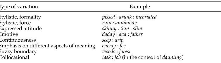
Table 1
Examples of near-synonym variations.
Type of variation Example
Stylistic, formality pissed:drunk:inebriated Stylistic, force ruin:annihilate
Expressed attitude skinny:thin:slim
Emotive daddy:dad:father
Continuousness seep:drip
Emphasis on different aspects of meaning enemy:foe
Fuzzy boundary woods:forest
Collocational task:job(in the context ofdaunting)
Writers often turn to such resources when confronted with a choice between near-synonyms, because choosing the wrong word can be imprecise or awkward or convey unwanted implications. These dictionaries are made for human use, and they are avail-able only on paper, not in electronic format.
Understanding the differences between near-synonyms is important for fine-grained distinctions in machine translation. For example, when translating the French word erreur to English, one of the near-synonymsmistake, blooper, blunder, boner, con-tretemps, error, faux pas, goof, slip, solecismcould be chosen, depending on the context and on the nuances that need to be conveyed. More generally, knowledge of near-synonyms is vital in natural language generation systems that take a nonlinguistic input (semantic representation) and generate text. When more than one word can be used, the choice should be based on some explicit preferences. Another application is an intelligent thesaurus, which would assist writers not only with lists of possible synonyms but also with the nuances they carry (Edmonds 1999).
1.1 Distinctions among Near-Synonyms
Near-synonyms can vary in many ways. DiMarco, Hirst, and Stede (1993) analyzed the types of differences adduced in dictionaries of near-synonym discrimination. They found that there was no principled limitation on the types, but a small number of types occurred frequently. A detailed analysis of the types of variation is given by Edmonds (1999). Some of the most relevant types of distinctions, with examples from CTRW, are presented below.
Denotational distinctionsNear-synonyms can differ in thefrequencywith which they express a component of their meaning (e.g.,Occasionally,invasionsuggests a large-scale but unplannedincursion), in thelatency(orindirectness) of the expression of the component (e.g., Teststrongly implies an actual application of these means), and in fine-grained variations of the idea itself (e.g., Paternalistic may suggest either benevolent rule or a style of government determined to keep the governed helpless and dependent). The frequency is signaled in the explanations in CTRW by words such as always, usually, sometimes,seldom,never. The latency is signaled by many words, including the obvious wordssuggests,denotes,implies, andconnotes. The strength of a distinction is signaled by words such asstronglyandweakly.
Figure 1
An excerpt fromChoose the Right Word(CTRW) by S. I. Hayakawa. Copyright ©1987. Reprinted by arrangement with HarperCollins Publishers, Inc.
praise common in such writing.Placidmay have an unfavorable connotation in suggesting an unimaginative, bovine dullness of personality.
Stylistic distinctions Stylistic variations of near-synonyms concern their level of formality, concreteness, force, floridity, and familiarity (Hovy 1990). Only the first three of these occur in CTRW. A sentence in CTRW expressing stylistic distinctions is this: Assistant and helperare nearly identical except for the latter’s greater informality. Words that signal the degree of formality includeformal,informal,formality, andslang. The degree ofconcretenessis signaled by words such asabstract,concrete, andconcretely. Force can be signaled by words such asemphaticandintensification.
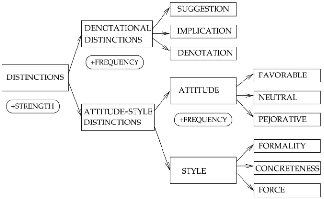
distinctions presented in Figure 2. The top-level classDISTINCTIONSconsists of DENO-TATIONAL DISTINCTIONS,ATTITUDE, andSTYLE. The last two are grouped together in a classATTITUDE-STYLE DISTINCTIONSbecause they are expressed by similar syntactic constructions in the text of CTRW. Therefore the algorithm to be described in Section 2.2 will treat them together.
The leaf classes ofDENOTATIONAL DISTINCTIONSare SUGGESTION, IMPLICATION, and DENOTATION; those of ATTITUDE are FAVORABLE, NEUTRAL, and PEJORATIVE; those ofSTYLEare FORMALITY, CONCRETENESS, and FORCE. All these leaf nodes have the attributeSTRENGTH, which takes the valueslow,medium, andhigh. All the leaf nodes except those in the classSTYLEhave the attributeFREQUENCY, which takes the values always, usually, sometimes,seldom, andnever. The DENOTATIONAL DISTINCTIONS have an additional attribute: the peripheral concept that is suggested, implied, or denoted.
1.2 The Clustered Model of Lexical Knowledge
Hirst (1995) and Edmonds and Hirst (2002) show that current models of lexical knowledge used in computational systems cannot account well for the properties of near-synonyms.
[image:4.486.48.378.423.626.2]The conventional view is that the denotation of a lexical item is represented as a concept or a structure of concepts (i.e., a word sense is linked to the concept it lexicalizes), which are themselves organized into an ontology. The ontology is often language independent, or at least language neutral, so that it can be used in multilin-gual applications. Words that are nearly synonymous have to be linked to their own slightly different concepts. Hirst (1995) showed that such a model entails an awkward taxonomic proliferation of language-specific concepts at the fringes, thereby defeating the purpose of a language-independent ontology. Because this model defines words
Figure 2
in terms of necessary and sufficient truth conditions, it cannot account for indirect expressions of meaning or for fuzzy differences between near-synonyms.
Edmonds and Hirst (2002) modified this model to account for near-synonymy. The meaning of each word arises out of a dependent combination of a context-independent denotation and a set of explicit differences from its near-synonyms, much as in dictionaries of near-synonyms. Thus the meaning of a word consists both of necessary and sufficient conditions that allow the word to be selected by a lexical choice process and a set of nuances of indirect meaning that may be conveyed with different strengths. In this model, a conventional ontology is cut off at a coarse grain and the near-synonyms are clustered under a shared concept, rather than linking each word to a separate concept. The result is aclustered model of lexical knowledge. Thus, each cluster has a core denotation that represents the essential shared denotational meaning of its near-synonyms. The internal structure of a cluster is complex, representing semantic (or denotational), stylistic, and expressive (or attitudinal) differences between the near-synonyms. The differences or lexical nuances are expressed by means of peripheral concepts (for denotational nuances) or attributes (for nuances of style and attitude).
The clustered model has the advantage that it keeps the ontology language neutral by representing language-specific distinctions inside the cluster of near-synonyms. The near-synonyms of a core denotation in each language do not need to be in separate clusters; they can be part of one larger cross-linguistic cluster.
However, building such representations by hand is difficult and time-consuming, and Edmonds and Hirst (2002) completed only nine of them. Our goal in the present work is to build a knowledge base of these representations automatically by extracting the content of all the entries in a dictionary of near-synonym discrimination. Un-like lexical resources such as WordNet (Miller 1995), in which the words in synsets are considered “absolute” synonyms, ignoring any differences between them, and thesauri such as Roget’s (Roget 1852) and Macquarie (Bernard 1987), which contain hierarchical groups of similar words, the knowledge base will include, in addition to the words that are near-synonyms, explicit explanations of differences between these words.
2. Building a Lexical Knowledge Base of Near-Synonym Differences
As we saw in Section 1, each entry in a dictionary of near-synonym discrimination lists a set of near-synonyms and describes the differences among them. We will use the termclusterin a broad sense to denote both the near-synonyms from an entry and their differences. Our aim is not only to automatically extract knowledge from one such dictionary in order to create a lexical knowledge base of near-synonyms (LKB of NS), but also to develop a general method that could be applied to any such dictionary with minimal adaptation. We rely on the hypothesis that the language of the entries contains enough regularity to allow automatic extraction of knowledge from them. Earlier versions of our method were described by Inkpen and Hirst (2001).
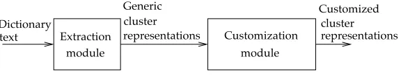
Figure 3
The two modules of the task.
strings from the generic clusters into concepts in the particular ontology. An example of a customization module will be described in Section 6.
The dictionary that we use is Choose the Right Word (Hayakawa 1994) (CTRW),1 which was introduced in Section 1. CTRW contains 909 clusters, which group 5,452 near-synonyms (more precisely, near-synonym senses, because a word can be in more than one cluster) with a total of 14,138 sentences (excluding examples of usage), from which we derive the lexical knowledge base. An example of the results of this phase, corresponding to the second, third, and fourth sentence for theabsorbcluster in Figure 1, is presented in Figure 4.
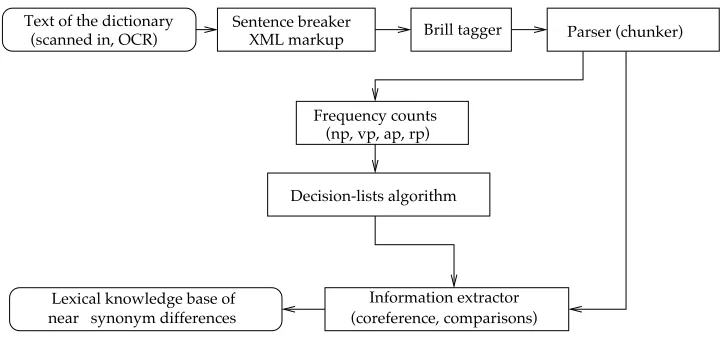
This section describes the extraction module, whose architecture is presented in Figure 5. It has two main parts. First, it learns extraction patterns; then it applies the patterns to extract differences between near-synonyms.
2.1 Preprocessing the Dictionary
After OCR scanning of CTRW and error correction, we used XML markup to segment the text of the dictionary into cluster name, cluster identifier, members (the synonyms in the cluster), entry (the textual description of the meaning of the near-synonyms and of the differences among them), cluster’s part of speech, cross-references to other clusters, and antonyms list. Sentence boundaries were detected by using general heuristics, plus heuristics specific for this particular dictionary; for example, examples appear in square brackets and after a colon.
2.2 The Decision-List Learning Algorithm
Before the system can extract differences between near-synonyms, it needs to learn extraction patterns. For each leaf class in the hierarchy (Figure 2) the goal is to learn a set of words and expressions from CTRW—that is, extraction patterns—that charac-terizes descriptions of the class. Then, during the extraction phase, for each sentence (or fragment of a sentence) in CTRW the program will decide which leaf class is expressed, with what strength, and what frequency. We use a decision-list algorithm to learn sets of words and extraction patterns for the classes DENOTATIONAL DISTINCTIONS and ATTITUDE-STYLE DISTINCTIONS. These are split further for each leaf class, as explained in Section 2.3.
The algorithm we implemented is inspired by the work of Yarowsky (1995) on word sense disambiguation. He classified the senses of a word on the basis of other words that the given word co-occurs with. Collins and Singer (1999) classified proper names
Figure 4
Example of distinctions extracted from CTRW.
as PERSON, ORGANIZATION, or LOCATIONusing contextual rules (that rely on other words appearing in the context of the proper names) and spelling rules (that rely on words in the proper names). Starting with a few spelling rules (using some proper-name features) in the decision list, their algorithm learns new contextual rules; using these rules, it then learns more spelling rules, and so on, in a process of mutual bootstrapping. Riloff and Jones (1999) learned domain-specific lexicons and extraction patterns (such asshot inxfor the terrorism domain). They used a mutual bootstrapping technique to alternately select the best extraction pattern for a category and add its extractions to the semantic lexicon; the newly added entries in the lexicon help in the selection of the next best extraction pattern.
Our decision-list (DL) algorithm (Figure 6) is tailored for extraction from CTRW. Like the algorithm of Collins and Singer (1999), it learns two different types of rules: Main rules are for words that are significant for distinction classes;auxiliary rules are for frequency words, strength words, and comparison words. Mutual bootstrapping in the algorithm alternates between the two types. The idea behind the algorithm is that starting with a few main rules (seed words), the program selects examples containing them and learns a few auxiliary rules. Using these, it selects more examples and learns new main rules. It keeps iterating until no more new rules are learned.
[image:7.486.53.416.467.636.2]The rules that the program learns are of the form x→h(x), meaning that word x is significant for the given class with confidence h(x). All the rules for that class form a decision list that allows us to compute the confidence with which new patterns
Figure 5
Figure 6
The decision-list learning algorithm.
are significant for the class. The confidence h(x) for a word x is computed with the formula:
h(x)= count(x,E )+α
count(x,E)+kα (1)
whereE is the set of patterns selected for the class, andEis the set of all input data. So, we count how many timesxis in the patterns selected for the class versus the total number of occurrences in the training data. Following Collins and Singer (1999),k= 2, because there are two partitions (relevant and irrelevant for the class).α=0.1 is a smoothing parameter.
than t times in the text of the dictionary (where t=3 in our experiments). Phrases that occur very few times are not likely to be significant patterns and eliminating them makes the process faster (fewer iterations are needed).
We apply the DL algorithm for each of the classes DENOTATIONAL DISTINCTIONS and ATTITUDE-STYLE DISTINCTIONS. The input to the algorithm is as follows: the set E of all chunks, the main seed words, and the restrictions on the part of speech of the words in main and auxiliary rules. For the class DENOTATIONAL DISTINCTIONS the main seed words are suggest, imply, denote,mean,designate,connote; the words in main rules are verbs and nouns, and the words in auxiliary rules are adverbs and modals. For the classATTITUDE-STYLE DISTINCTIONSthe main seed words areformal, informal,pejorative,disapproval,favorable,abstract,concrete; the words in main rules are adjectives and nouns, and the words in auxiliary rules are adverbs. For example, for the classDENOTATIONAL DISTINCTIONS, starting with the rulesuggest→0.99, the program selects examples such as these (where the numbers give the frequency in the training data):
[vx [md can] [vb suggest]]--150 [vx [rb sometimes] [vb suggest]]--12
Auxiliary rules are learned for the wordssometimesandcan, and using these rules, the program selects more examples such as these:
[vx [md can] [vb refer]]--268
[vx [md may] [rb sometimes] [vb imply]]--3
From these, new main rules are learned for the wordsreferandimply. With these rules, more auxiliary rules are selected—for the wordmayand so on.
The ATTITUDEand STYLE classes had to be considered together because both of them use adjectival comparisons. Examples ofATTITUDE-STYLE DISTINCTIONSclass are these:
[ax [rbs most] [jj formal]]--54
[ax [rb much] [more more] [jj formal]]--9 [ax [rbs most] [jj concrete]]--5
2.3 Classification and Extraction
After we run the DL algorithm for the class DENOTATIONAL DISTINCTIONS, we split the words in the list of main rules into its three sub-classes, as shown in Figure 2. This sub-classification is manual for lack of a better procedure. Furthermore, some words can be insignificant for any class (e.g., the wordalso) or for the given class; during the sub-classification we mark them as OTHER. We repeat the same procedure for frequencies and strengths with the words in the auxiliary rules. The words marked asOTHERand the patterns that do not contain any word from the main rules are ignored in the next processing steps. Similarly, after we run the algorithm for the class ATTITUDE-STYLE DISTINCTIONS, we split the words in the list of main rules into its sub-classes and sub-sub-classes (Figure 2). Frequencies are computed from the auxiliary rule list, and strengths are computed by a module that resolves comparisons.
tries to extract one or more pieces of knowledge from it. Examples of results after this stage are presented in Figure 4. The information extracted for denotational distinctions is the near-synonym itself, the class, frequency, and strength of the distinction, and the peripheral concept. At this stage, the peripheral concept is a string extracted from the sentence. Strength takes the valuelow,medium, orhigh; frequency takes the value always,usually,sometimes,seldom, ornever. Default values (usuallyand medium) are used when the strength or the frequency are not specified in the sentence. The information extracted for attitudinal and stylistic distinctions is analogous.
The extraction program considers what near-synonyms each sentence fragment is about (most often expressed as the subject of the sentence), what the expressed distinc-tion is, and with what frequency and relative strength. If it is a denotadistinc-tional distincdistinc-tion, then the peripheral concept involved has to be extracted too (from the object position in the sentence). Therefore, our program looks at the subject of the sentence (the first noun phrase before the main verb) and the object of the sentence (the first noun phrase after the main verb). This heuristic works for sentences that present one piece of information. There are many sentences that present two or more pieces of information. In such cases, the program splits a sentence into coordinated clauses (or coordinated verb phrases) by using a parser (Collins 1996) to distinguish when a coordinating conjunction (and,but, whereas) is conjoining two main clauses or two parts of a complex verb phrase. From 60 randomly selected sentences, 52 were correctly dealt with (41 needed no split, 11 were correctly split). Therefore, the accuracy was 86.6%. The eight mistakes included three sentences that were split but should not have been, and five that needed splitting but were not. The mistakes were mainly due to wrong parse trees.
When no information is extracted in this way, a few general patterns are matched with the sentence in order to extract the near-synonyms; an example of such pattern is: To NS1 is to NS2 .... There are also heuristics to retrieve compound subjects of the form near-syn and near-syn and near-syn, near-syn, and near-syn. Once the class is determined to be either DENOTATIONAL DISTINCTIONSor ATTITUDE-STYLE DISTINC-TIONS, the target class (one of the leaves in the class hierarchy in Figure 2) is deter-mined by using the manual partitions of the rules in the main decision list of the two classes.
Sometimes the subject of a sentence refers to a group of near-synonyms. For ex-ample, if the subject is the remaining words, our program needs to assert information about all the near-synonyms from the same cluster that were not yet mentioned in the text. In order to implement coreference resolution, we applied the same DL algorithm to retrieve expressions used in CTRW to refer to synonyms or groups of near-synonyms.
Sometimes CTRW describes stylistic and attitudinal distinctions relative to other near-synonyms in the cluster. Such comparisons are resolved in a simple way by consid-ering only three absolute values:low,medium,high. We explicitly tell the system which words represent what absolute values of the corresponding distinction (e.g.,abstractis at the low end ofConcreteness) and how the comparison terms increase or decrease the absolute value (e.g.,less abstractcould mean amediumvalue ofConcreteness).
2.4 Evaluation
In order to evaluate the final results, we randomly selected 25 clusters as a de-velopment set, and another 25 clusters as a test set. The dede-velopment set was used to tune the program by adding new patterns if they helped improve the results. The test set was used exclusively for testing. We built by hand a standard solution for each set. The baseline algorithm is to choose the default values whenever possible. There are no defaults for the near-synonyms the sentence is about or for peripheral concepts; therefore, for these, the baseline algorithm assigns the sentence subject and object, respectively, using only tuples extracted by the chunker.
The measures that we used for evaluating each piece of information extracted from a sentence fragment wereprecisionandrecall. The results to be evaluated have four com-ponents forATTITUDE-STYLE DISTINCTIONSand five components for DENOTATIONAL DISTINCTIONS. There could be missing components (except strength and frequency, which take default values). Precision is the total number of correct components found (summed over all the sentences in the test set) divided by the total number of com-ponents found. Recall is the total number of correct comcom-ponents found divided by the number of components in the standard solution.
For example, for the sentenceSometimes, however,profitcan refer to gains outside the context of moneymaking, the program obtains profit, usually, medium, Denotation, gains outside the context of moneymaking, whereas the solution isprofit, some-times,medium,Denotation,gains outside the context of money-making. The pre-cision is .80 (four correct out of five found), and the recall is also .80 (four correct out of five in the standard solution).
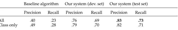
Table 2 presents the results of the evaluation.2 The first row of the table presents the results as a whole (all the components of the extracted lexical knowledge base). Our system increases precision by 36 percentage points and recall by 46 percentage points over baseline on the development set.3Recall and precision are both slightly higher still on the test set; this shows that the patterns added during the development stage were general.
The second row of the table gives the evaluation results for extracting only the class of the distinction expressed, ignoring the strengths, frequencies, and peripheral concepts. This allows for a more direct evaluation of the acquired extraction patterns. The baseline algorithm attained higher precision than in the case when all the com-ponents are considered because the default class Denotation is the most frequent in CTRW. Our algorithm attained slightly higher precision and recall on the development set than it did in the complete evaluation, probably due to a few cases in which the frequency and strength were incorrectly extracted, and slightly lower on the test set, probably due to some cases in which the frequency and strength were easy to extract correctly.
2.5 Conclusion
The result of this stage is a generic lexical knowledge base of near-synonym differences. In subsequent sections, it will be enriched with knowledge from other sources; informa-tion about the collocainforma-tional behavior of the near-synonyms is added in Secinforma-tion 3, and
2 The improvement over the baseline is statistically significant (atp= 0.005 level or better) for all the results presented in this article, except in one place to be noted later. Statistical significance tests were done with the pairedttest, as described by Manning and Sch ¨utze (1999, pages 208–209).
Table 2
Precision and recall of the baseline and of our algorithm (for all the components and for the distinction class only; boldface indicates best results).
Baseline algorithm Our system (dev. set) Our system (test set)
Precision Recall Precision Recall Precision Recall
All .40 .23 .76 .69 .83 .73
Class only .49 .28 .79 .70 .82 .71
more distinctions acquired from machine-readable dictionaries are added in Section 4. To be used in a particular NLP system, the generic LKB of NS needs to be customized (Section 6). Section 7 shows how the customized LKB of NS can actually be used in Natural Language Generation (NLG).
The method for acquiring extraction patterns can be applied to other dictionaries of synonym differences. The extraction patterns that we used to build our LKB of NS are general enough to work on other dictionaries of English synonyms. To verify this, we applied the extraction programs presented in Section 2.3, without modification, to the usage notes in theMerriam-Webster Online Dictionary.4The distinctions expressed in these usage notes are similar to the explanations from CTRW, but the text of these notes is shorter and simpler. In a sample of 100 usage notes, we achieved a precision of 90% and a recall of 82%.
3. Adding Collocational Knowledge from Free Text
In this section, the lexical knowledge base of near-synonym differences will be enriched with knowledge about the collocational behavior of the near-synonyms. We take col-locations here to be pairs of words that appear together, consecutively or separated by only a few non-content words, much more often than by chance. Our definition is purely statistical, and we make no claim that the collocations that we find have any element of idiomaticity; rather, we are simply determining the preferences of our near-synonyms for combining, or avoiding combining, with other words. For exampledaunting taskis a preferred combination (a collocation, in our terms), whereasdaunting jobis less preferred (it should not be used in lexical choice unless there is no better alternative), anddaunting dutyis ananti-collocation(Pearce 2001) that sounds quite odd and must not be used in lexical choice.
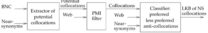
There are three main steps in acquiring this knowledge, which are shown in Fig-ure 7. The first two look in free text—first the British National Corpus, then the World Wide Web—for collocates of all near-synonyms in CTRW, removing any closed-class words (function words). For example, the phrasedefeat the enemywill be treated asdefeat enemy; we will refer to such pairs as bigrams, even if there were intervening words. The third step uses the t-test (Church et al. 1991) to classify less frequent or unobserved bigrams as less preferred collocations or anti-collocations. We outline the three steps below; a more-detailed discussion is presented by Inkpen and Hirst (2002).
Figure 7
The three steps in acquiring collocational knowledge for near-synonyms.
3.1 Extracting Collocations from the British National Corpus
In step 1 of our procedure, our data was the 100-million-word part-of-speech-tagged British National Corpus (BNC).5Only 2.61% of the near-synonyms are absent from the BNC; and only 2.63% occur between one and five times. We first preprocessed the BNC by removing all words tagged as closed-class and all the proper names, and then used the Ngram Statistics Package6(Pedersen and Banerjee 2003), which counts bigram (or
n-gram) frequencies in a corpus and computes various statistics to measure the degree of association between two words: pointwise mutual information (MI), Dice, chi-square (χ2), log-likelihood (LL), and Fisher’s exact test. (See Manning and Sch ¨utze [1999] for a review of statistical methods that can be used to identify collocations.)
Because these five measures rank potential collocations in different ways and have different advantages and drawbacks, we decided to combine them by choosing as a collocation any bigram that was ranked by at least two of the measures as one of that measure’s T most-highly ranked bigrams; the threshold T may differ for each measure. Lower values for T increase the precision (reduce the chance of accepting noncollocations) but may not get many collocations for some of the near-synonyms; higher values increase the recall at the expense of lower precision. Because there is no principled way of choosing these values, we opted for higher recall, with step 2 of the process (Section 3.2) filtering out many noncollocations in order to increase the precision. We took the first 200,000 bigrams selected by each measure, except for Fisher’s measure for which we took all 435,000 that were ranked equal top. From these lists, we retained only those bigrams in which one of the words is a near-synonym in CTRW.7
5 http://www.hcu.ox.ac.uk/BNC/
6 http://www.d.umn.edu/∼tpederse/nsp.html. We used version 0.4, known at the time as the Bigram Statistics Package (BSP).
7 Collocations of a near-synonym with the wrong part of speech were not considered (the collocations are tagged), but when a near-synonym has more than one major sense, collocations for senses other than the one required in the cluster could be retrieved. For example, for the clusterjob, task, duty, and so on, the collocationimport dutyis likely to be for a different sense ofduty(the tariff sense). Therefore
disambiguation is required (assuming one sense per collocation). We experimented with a simple Lesk-style method (Lesk 1986). For each collocation, instances from the corpus were retrieved, and the content words surrounding the collocations were collected. This set of words was then intersected with the entry for the near-synonym in CTRW. A non-empty intersection suggests that the collocation and the entry use the near-synonym in the same sense. If the intersection was empty, the collocation was not retained. However, we ran the disambiguation algorithm only for a subset of CTRW, and then abandoned it, because hand-annotated data are needed to evaluate how well it works and because it was very time-consuming (due to the need to retrieve corpus instances for each collocation). Moreover, skipping disambiguation is relatively harmless because including these wrong senses in the final lexical
3.2 Filtering with Mutual Information from Web Data
In the previous step we emphasized recall at the expense of precision: Because of the relatively small size of the BNC, it is possible that the classification of a bigram as a collocation in the BNC was due to chance. However, the World Wide Web (the portion indexed by search engines) is big enough that a result is more reliable. So we can use frequency on the Web to filter out the more dubious collocations found in the previous step.8We did this for each putative collocation by counting its occurrence on the Web, the occurrence of each component word, and computing the pointwise mutual information (PMI) between the words. Only those whose pointwise mutual information exceeded a thresholdTpmiwere retained.
More specifically, ifwis a word that collocates with one of the near-synonymsxin a cluster, a proxy PMIproxfor the pointwise mutual information between the words can be given by the ratio
P(w,x) P(x) =
nwx
nx
where nwx and nx are the number of occurrences of wx and x, respectively. The
for-mula does not include P(w) because it is the same for various x. We used an inter-face to the AltaVista search engine to do the counts, using the number of hits (i.e., matching documents) as a proxy for the actual number of bigrams.9 The threshold
Tpmi for PMIprox was determined empirically by finding the value that optimized re-sults on a standard solution, constructed as follows. We selected three clusters from CTRW, with a total of 24 near-synonyms. For these, we obtained 916 candidate collo-cations from the BNC. Two human judges (computational linguistics students, native speakers of English) were asked to mark the true collocations (what they considered to be good usage in English). The candidate pairs were presented to the judges in random order, and each was presented twice.10 A bigram was considered to be a true collocation only if both judges considered it so. We used this standard solution to choose the value of Tpmi that maximizes the accuracy of the filtering program. Accuracy on the test set was 68.3% (compared to approximately 50% for random choice).
3.3 Finding Less Preferred Collocations and Anti-Collocations
In seeking knowledge of less preferred collocations and anti-collocations, we are look-ing for bigrams that occur infrequently or not at all. The low frequency or absence of a
8 Why not just use the Web and skip the BNC completely? Because we would then have to count Web occurrences of every near-synonym in CTRW combined with every content word in English. Using the BNC as a first-pass filter vastly reduces the search space.
9 The collocations were initially acquired from the BNC with the right part of speech for the near-synonym because the BNC is part-of-speech-tagged, but on the Web there are no part-of-speech tags; therefore a few inappropriate instances may be included in the counts.
bigram in the BNC may be due to chance. However, the World Wide Web is big enough that a negative result is more reliable. So we can again use frequency on the Web—this time to determine whether a bigram that was infrequent or unseen in the BNC is truly a less preferred collocation or anti-collocation.
The bigrams of interest now are those in which collocates for a near-synonym that were found in step 1 and filtered in step 2 are combined with another member of the same near-synonym cluster. For example, if the collocation daunting task was found, we now look on the Web for the apparent noncollocationsdaunting job, daunting duty, and other combinations of daunting with near-synonyms of task. A low number of co-occurrences indicates a less preferred collocation or anti-collocation. We employ the t-test, following Manning and Sch ¨utze (1999, pages 166–168), to look for differences.
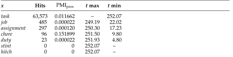
The collocations of each near-synonym with a given collocate are grouped in three classes, depending on thetvalues of pairwise collocations. Atvalue comparing each collocation and the collocation with maximum frequency is computed, and so is the tvalue between each collocation and the collocation with minimum frequency. Table 3 presents an example.
[image:15.486.52.442.567.663.2]After thet-test scores were computed, a set of thresholds was determined to classify the collocations in the three groups: preferred collocations, less preferred collocations, and anti-collocations. Again, we used a standard solution in the procedure. Two judges manually classified a sample of 2,838 potential collocations obtained for the same three clusters of near-synonyms from 401 collocations that remained after filtering. They were instructed to mark as preferred collocations all the potential collocations that they considered good idiomatic use of language, as anti-collocations the ones that they would not normally use, and as less preferred collocations the ones that they were not comfortable classifying in either of the other two classes. When the judges agreed, the class was clear. When they did not agree, we used simple rules, such as these: When one judge chose the class-preferred collocation, and the other chose the class anti-collocation, the class in the solution was less preferred collocation (because such cases seemed to be difficult and controversial); when one chose preferred collocation, and the other chose less preferred collocation, the class in the solution was preferred collocation; when one chose anti-collocation, and the other chose less preferred collocation, the class in the solution was anti-collocation. The agreement between judges was 84%,κ=0.66 (with a 95% confidence interval of 0.63 to 0.68).
Table 3
Example of counts, mutual information scores, andt-test scores for the collocatedauntingwith near-synonyms oftask. The second column shows the number of hits for the collocationdaunting x, wherexis the near-synonym in the first column. The third column shows PMIprox(scaled by 105for readability), the fourth column, thetvalues between the collocation with maximum frequency (daunting task) anddaunting x, and the last column, thet-test betweendaunting xand the collocations with minimum frequency (daunting stintanddaunting hitch).
x Hits PMIprox tmax tmin task 63,573 0.011662 – 252.07 job 485 0.000022 249.19 22.02 assignment 297 0.000120 250.30 17.23
chore 96 0.151899 251.50 9.80
duty 23 0.000022 251.93 4.80
stint 0 0 252.07 –
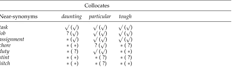
Table 4
Example of results of our program for collocations of near-synonyms in thetaskcluster.√marks preferred collocations, ? marks less preferred collocations, and∗marks anti-collocations. The combined opinion of the judges about the same pairs of words is shown in parentheses.
Collocates
Near-synonyms daunting particular tough
task √(√) √(√) √(√)
job ? (√) √(√) √(√)
assignment ∗(√) √(√) √(√)
chore ∗(∗) ? (√) ∗( ?)
duty ∗( ?) √(√) ∗(∗)
stint ∗(∗) ∗( ?) ∗( ?)
hitch ∗(∗) ∗( ?) ∗(∗)
We used this standard solution as training data to C4.511 to learn a decision tree for the three-way classifier. The features in the decision tree are the t-test between each collocation and the collocation from the same group that has maximum frequency on the Web, and the t-test between the current collocation and the collocation that has minimum frequency (as presented in Table 3). We did 10-fold cross-validation to estimate the accuracy on unseen data. The average accuracy was 84.1%, with a standard error of 0.5%; the baseline of always choosing the most frequent class, anti-collocations, yields 71.4%. We also experimented with including PMIproxas a feature in the decision tree, and with manually choosing thresholds (without a decision tree) for the three-way classification, but the results were poorer. The three-three-way classifier can fix some of the mistakes of the PMI filter: If a wrong collocation remains after the PMI filter, the classifier can classify it in the anti-collocations class. We conclude that the acquired collocational knowledge has acceptable quality.
3.4 Results
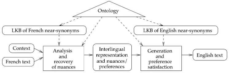
We obtained 1,350,398 distinct bigrams that occurred at least four times. We selected col-locations for all 909 clusters in CTRW (5,452 near-synonyms in total). Table 4 presents an example of results for collocational classification of bigrams, where√marks preferred collocations, ? marks less preferred collocations, and ∗ marks anti-collocations. This gave us a lexical knowledge base of near-synonym collocational behavior. An example of collocations extracted for the near-synonymtaskis presented in Table 5, where the columns are, in order, the name of the measure, the rank given by the measure, and the value of the measure.
4. Adding Knowledge from Machine-Readable Dictionaries
Information about near-synonym differences can be found in other types of dictionaries besides those explicitly on near-synonyms. Although conventional dictionaries, unlike CTRW, treat each word in isolation, they may nonetheless contain useful information
Table 5
Example of collocations extracted for the near-synonymtask. The first collocation was selected (ranked in the set of firstTcollocations) by four measures; the second collocation was selected by two measures.
Collocation Measure Rank Score
daunting/A task/N MI 24,887 10.85
LL 5,998 907.96
χ2 16,341 122,196.82
Dice 2,766 0.02
repetitive/A task/N MI 64,110 6.77
χ2 330,563 430.40
about near-synonyms because some definitions express a distinction relative to another near-synonym. From the SGML-marked-up text of theMacquarie Dictionary12(Delbridge et al. 1987), we extracted the definitions of the near-synonyms in CTRW for the expected part of speech that contained another near-synonym from the same cluster. For example, for the CTRW clusterburlesque, caricature, mimicry, parody, takeoff, travesty, one definition extracted for the near-synonymburlesquewasany ludicrous take-off or debasing caricature because it contains caricature from the same cluster. A series of patterns was used to extract the difference between the two near-synonyms wherever possible. For the burlesqueexample, the extracted information was
burlesque,usually,medium,Denotation,ludicrous, burlesque,usually,medium,Denotation,debasing.
The number of new denotational distinctions acquired by this method was 5,731. We also obtained additional information from the General Inquirer13 (Stone et al. 1966), a computational lexicon that classifies each word in it according to an extendable number of categories, such as pleasure, pain, virtue, and vice; overstatement and un-derstatement; and places and locations. The category of interest here isPositiv/Negativ. There are 1,915 words marked asPositiv(not including words foryes, which is a separate category of 20 entries), and 2,291 words marked asNegativ(not including the separate category of no in the sense of refusal). For each near-synonym in CTRW, we used this information to add a favorable or unfavorable attitudinal distinction accordingly. If there was more than one entry (several senses) for the same word, the attitude was asserted only if the majority of the senses had the same marker. The number of attitudinal distinctions acquired by this method was 5,358. (An attempt to use the occasional markers for formality in WordNet in a similar manner resulted in only 11 new distinctions.)
As the knowledge from each source is merged with the LKB, it must be checked for consistency in order to detect conflicts and resolve them. The algorithm for resolving conflicts is a voting scheme based on the intuition that neutral votes should have less weight than votes for the two extremes. The algorithm outputs a list of the conflicts and a proposed solution. This list can be easily inspected by a human, who can change
Figure 8
Fragment of the representation of theerrorcluster (prior to customization).
the solution of the conflict in the final LKB of NS, if desired. The consistency-checking program found 302 conflicts for the merged LKB of 23,469 distinctions. After conflict resolution, 22,932 distinctions remained. Figure 8 shows a fragment of the knowledge extracted for the near-synonyms oferrorafter merging and conflict resolution.
5. Related Work
5.1 Building Lexical Resources
Lexical resources for natural language processing have also been derived from other dictionaries and knowledge sources. The ACQUILEX14 Project explored the utility of constructing a multilingual lexical knowledge base (LKB) from machine-readable ver-sions of conventional dictionaries. Ide and V´eronis (1994) argue that it is not possible to build a lexical knowledge base from a machine-readable dictionary (MRD) because the information it contains may be incomplete, or it may contain circularities. It is possible to combine information from multiple MRDs or to enhance an existing LKB, they say, although human supervision may be needed.
Automatically extracting world knowledge from MRDs was attempted by projects such as MindNet at Microsoft Research (Richardson, Dolan, and Vanderwende 1998), and Barri`erre and Popowich’s (1996) project, which learns from children’s dictionaries. IS-A hierarchies have been learned automatically from MRDs (Hearst 1992) and from corpora (Caraballo [1999] among others).
Research on merging information from various lexical resources is related to the present work in the sense that the consistency issues to be resolved are similar. One example is the construction of Unified Medical Language System (UMLS)15(Lindberg, Humphreys, and McCray 1993), in the medical domain. UMLS takes a wide range of lexical and ontological resources and brings them together as a single resource. Most of this work is done manually at the moment.
5.2 Acquiring Collocational Knowledge
There has been much research on extracting collocations for different applications. Like Church et al. (1991), we use the t-test and mutual information (MI), but unlike them we use the Web as a corpus for this task (and a modified form of mutual information), and we distinguish three types of collocations. Pearce (2001) improved the quality of retrieved collocations by using synonyms from WordNet (Pearce 2001); a pair of words was considered a collocation if one of the words significantly prefers only one (or several) of the synonyms of the other word. For example, emotional baggageis a good collocation becausebaggage andluggageare in the same synset and∗emotional luggage is not a collocation. Unlike Pearce, we use a combination of t-test and MI, not just frequency counts, to classify collocations.
There are two typical approaches to collocations in previous NLG systems: the use of phrasal templates in the form of canned phrases, and the use of automatically extracted collocations for unification-based generation (McKeown and Radev 2000). Statistical NLG systems (such as Nitrogen [Langkilde and Knight 1998]) make good use of the most frequent words and their collocations, but such systems cannot choose a less-frequent synonym that may be more appropriate for conveying desired nuances of meaning if the synonym is not a frequent word.
Turney (2001) used mutual information to choose the best answer to questions about near-synonyms in the Test of English as a Foreign Language (TOEFL) and English as a Second Language (ESL). Given a problem word (with or without context) and four alternative words, the question is to choose the alternative most similar in meaning to the problem word (the problem here is to detect similarities, whereas in our work differences are detected). His work is based on the assumption that two synonyms are likely to occur in the same document (on the Web). This can be true if the author needs to avoid repeating the same word, but not true when the synonym is of secondary importance in a text. The alternative that has the highest pointwise mutual information for information retrieval (PMI-IR) with the problem word is selected as the answer. We used the same measure in Section 3.3—the mutual information between a collocation and a collocate that has the potential to discriminate between near-synonyms. Both works use the Web as a corpus, and a search engine to estimate the mutual information scores.
5.3 Near-Synonyms
As noted in the introduction, our work is based on that of Edmonds and Hirst (2002) and Hirst (1995), in particular the model for representing the meaning of the near-synonyms presented in Section 1.2 and the preference satisfaction mechanism used in Section 7.
Other related research involving differences between near-synonyms has a lin-guistic or lexicographic, rather than computational, flavor. Apresjan built a bilin-gual dictionary of synonyms, more specifically a dictionary of English synonyms explained in Russian (Apresjan et al. 1980). It contains 400 entries selected from the approximately 2,500 entries from Webster’s New Dictionary of Synonyms, but re-organized by splitting or merging clusters of synonyms, guided by lexicographic principles described by Apresjan (2000). An entry includes the following types of differences: semantic, evaluative, associative and connotational, and differences in emphasis or logical stress. These differences are similar to the ones used in our work.
Gao (2001) studied the distinctions between near-synonym verbs, more specifically Chinese physical action verbs such as verbs of cutting, putting, throwing, touching, and lying. Her dissertation presents an analysis of the types of semantic distinctions relevant to these verbs, and how they can be arranged into hierarchies on the basis of their semantic closeness.
Ploux and Ji (2003) investigated the question of which words should be considered near-synonyms, without interest in their nuances of meaning. They merged clusters of near-synonyms from several dictionaries in English and French and represented them in a geometric space. In our work, the words that are considered near-synonyms are taken from CTRW; a different dictionary of synonyms may present slightly different views. For example, a cluster may contain some extra words, some missing words, or sometimes the clustering could be done in a different way. A different approach is to automatically acquire near-synonyms from free text. Lin et al. (2003) acquire words that are related by contextual similarity and then filter out the antonyms by using a small set of manually determined patterns (such as “either X or Y”) to construct Web queries for pairs of candidate words. The problem of this approach is that it still includes words that are in relations other than near-synonymy.
6. Customizing the Lexical Knowledge Base of Near-Synonym Differences
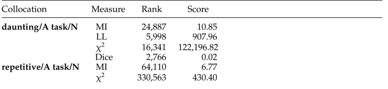
The initial LKB of NS built in Sections 2 to 4 is a general one, and it could, in principle, be used in any (English) NLP system. For example, it could be used in the lexical-analysis or lexical-choice phase of machine translation. Figure 9 shows that during the analysis phase, a lexical knowledge base of near-synonym differences in the source language is used, together with the context, to determine the set of nuances that are expressed in the source-language text (in the figure, the source language is French and the target language is English). In the generation phase, these nuances becomepreferencesfor the lexical-choice process. Not only must the target-language text express the same meaning as the source-language text (necessary condition), but the choice of words should satisfy thepreferencesas much as possible.
Figure 9
Lexical analysis and choice in machine translation; adapted from Edmonds and Hirst (2002). The solid lines show the flow of data: input, intermediate representations, and output; the dashed lines show the flow of knowledge from the knowledge sources to the analysis and the generation module. The rectangles denote the main processing modules; the rest of the boxes denote data or knowledge sources.
we modified the lexical-choice component of a preexisting NLG system, HALogen (Langkilde 2000; Langkilde and Knight 1998), to handle knowledge about the near-synonym differences. (Xenon will be described in detail in Section 7.) This required customization of the LKB to the Sensus ontology (Knight and Luk 1994) that HALogen uses as its representation.
Customization of the core denotations for Xenon was straightforward. The core denotation of a cluster is a metaconcept representing the disjunction of all the Sensus concepts that could correspond to the near-synonyms in a cluster. The names of meta-concepts, which must be distinct, are formed by the prefix generic, followed by the name of the first near-synonym in the cluster and the part of speech. For example, if the cluster islie, falsehood, fib, prevarication, rationalization, untruth, the name of the cluster is generic lie n.
Customizing the peripheral concepts, which are initially expressed as strings, could include parsing the strings and mapping the resulting syntactic representation into a semantic representation. For Xenon, however, we implemented a set of 22 simple rules that extract the actual peripheral concepts from the initial peripheral strings. A trans-formation rule takes a string of words part-of-speech tagged and extracts a main word, several roles, and fillers for the roles. The fillers can be words or recursive structures. In Xenon, the words used in these representations are not sense-disambiguated. Here are two examples of input strings and extracted peripheral concepts:
"an embarrassing breach of etiquette"
=> (C / breach :GPI etiquette :MOD embarrassing)
"to an embarrassing or awkward occurrence"
=> (C / occurrence :MOD (OR embarrassing awkward))
The roles used in these examples are MOD (modifier) and GPI (generalized possession inverse). The rules that were used for these two examples are these:
We evaluated our customization of the LKB on a hand-built standard solution for a set of peripheral strings: 139 strings to be used as a test set and 97 strings to be used as a development set. The rules achieved a coverage of 75% on the test set with an accuracy of 55%.16 In contrast, a baseline algorithm of taking the first word in each string as the peripheral concept covers 100% of the strings, but with only 16% accuracy.
Figure 10 shows the full customized representation for the near-synonyms oferror, derived from the initial representation that was shown earlier in Figure 8. (See Inkpen [2003] for more examples of customized clusters.) The peripheral concepts are factored out, and the list of distinctions contains pointers to them. This allows peripheral con-cepts to be shared by two or more near-synonyms.
7. Xenon: An NLG System that Uses Knowledge of Near-Synonym Differences This section presents Xenon, a large-scale NLG system that uses the lexical knowledge-base of near-synonyms customized in Section 6. Xenon integrates a new near-synonym choice module with the sentence realization system HALogen17 (Langkilde 2000; Langkilde and Knight 1998). HALogen is a broad-coverage general-purpose natural language sentence generation system that combines symbolic rules with linguistic information gathered statistically from large text corpora. The internal architecture of HALogen is presented in Figure 11. A forest of all possible sentences (combi-nations of words) for the input is built, and the sentences are then ranked ac-cording to an n-gram language model in order to choose the most likely one as output.
Figure 12 presents the architecture of Xenon. The input is a semantic representation and a set of preferences to be satisfied. The final output is a set of sentences and their scores. A concrete example of input and output is shown in Figure 13. Note that HALogen may generate some ungrammatical constructs, but they are (usually) assigned lower scores. The first sentence (the highest ranked) is considered to be the solution.
7.1 Metaconcepts
The semantic representation input to Xenon is represented, like the input to HAL-ogen, in an interlingua developed at University of Southern California/Information Sciences Institute (USC/ISI).18 As described by Langkilde-Geary (2002b), this lan-guage contains a specified set of 40 roles, whose fillers can be either words, con-cepts from Sensus (Knight and Luk 1994), or complex interlingual representations. The interlingual representations may be underspecified: If some information needed by HALogen is not present, it will use its corpus-derived statistical information to
16 We found that sometimes a rule would extract only a fragment of the expected configuration of concepts but still provided useful knowledge; however, such cases were not considered to be correct in this evaluation, which did not allow credit for partial correctness. For example, if the near-synonymcommand denotesthe/TD stated/VB demand/NN of/IN a/TD superior/JJ, the expected peripheral concept is (C1 / demand :GPI superior :MOD stated). If the program extracted only(C1 / demand :GPI superior), the result was not considered correct, but the information might still help in an NLP system. 17 http://www.isi.edu/licensed-sw/halogen/
Figure 10
The final representation of theerrorcluster.
make choices. Xenon extends this representation language by adding metaconcepts that correspond to the core denotation of the clusters of near-synonyms. For example, in Figure 13, the metaconcept is generic lie n. As explained in Section 6, metacon-cepts may be seen as a disjunction of all the senses of the near-synonyms of the cluster.
7.2 Near-Synonym Choice
Figure 11
The architecture of the sentence realizer HALogen.
the highest-ranked sentence. For example, the expanded representation of the input in Figure 13 is presented in Figure 14. The near-synonym choice module gives higher weight tofibbecause it satisfies the preferences better than the other near-synonyms in the cluster,lie, falsehood, fib, prevarication, rationalization,anduntruth.
7.3 Preferences and Similarity of Distinctions
The preferences that are input to Xenon could be given by the user, or they could come from an analysis module if Xenon is used in a machine translation system (correspond-ing to nuances of near-synonyms in a different language, see Figure 9). The preferences, like the distinctions expressed in the LKB of NS, are of three types: attitudinal, stylistic, and denotational. Examples of each:
(low formality) (disfavour :agent)
(imply (C / assessment :MOD ( M / (*OR* ignorant uninformed)).
The formalism for expressing preferences is from I-Saurus (Edmonds 1999). The preferences are transformed internally into pseudodistinctions that have the same form as the corresponding type of distinctions so that they can be directly compared with the distinctions. The pseudodistinctions corresponding to the previous examples are these:
(-− low Formality)
(- always high Pejorative :agent) (- always medium Implication
(C/assessment :MOD (M/(OR ignorant uninformed)).
Figure 12
[image:24.486.59.335.531.636.2]Figure 13
Example of input and output of Xenon.
Figure 14
The interlingual representation of the input in Figure 13 after expansion by the near-synonym choice module.
For each near-synonym NS in a cluster, a weight is computed by summing the degree to which the near-synonym satisfies each preference from the set P of input preferences:
Weight(NS,P)=
p∈P
Sat(p, NS). (2)
The weights are transformed through an exponential function so that numbers are comparable with the differences of probabilities from HALogen’s language model:
f(x)= ex
k
e−1. (3)
We setk=15 as a result of experiments with a development set.
For a given preferencep∈P, the degree to which it is satisfied by NS is reduced to computing the similarity between each of NS’s distinctions and a pseudodistinctiond(p) generated fromp. The maximum value overiis taken (wheredi(w) is theith distinction
of NS):
Sat(p, NS)=max
where the similarity of two distinctions, or of a distinction and a preference (trans-formed into a distinction), is computed with the three types of similarity measures that were used by Edmonds and Hirst (2002) in I-Saurus:
Sim(d1,d2)=
Simden(d1,d2) ifd1andd2are denotational distinctions Simatt(d1,d2) ifd1andd2are attitudinal distinctions Simsty(d1,d2) ifd1andd2are stylistic distinctions
0 otherwise
(5)
Distinctions are formed out of several components, represented as symbolic values on certain dimensions, such as frequency (seldom,sometimes, etc.) and strength (low, medium,high). In order to compute a numeric score, each symbolic value is mapped into a numeric one. The numeric values are not as important as their relative difference. If the two distinctions are not of the same type, they are incommensurate and their similarity is zero. The formulas for Simattand Simstyinvolve relatively straightforward matching. However, Simden requires the matching of complex interlingual structures. This boils down to computing the similarity between the main concepts of the two interlingual representations, and then recursively mapping the shared semantic roles (and compensating for the roles that appear in only one). When atomic concepts or words are reached, we use a simple measure of word/concept similarity based on the hierarchy of Sensus. All the details of these formulas, along with examples, are presented by Inkpen and Hirst (2003).
7.4 Integrating the Knowledge of Collocational Behavior
Knowledge of collocational behavior is not usually present in NLG systems. Adding it will increase the quality of the generated text, making it more idiomatic: The system will give priority to a near-synonym that produces a preferred collocation and will not choose one that causes an anti-collocation to appear in the generated sentence.
Unlike most other NLG systems, HALogen already incorporates some collocational knowledge implicitly encoded in its language model (bigrams or trigrams), but this is mainly knowledge of collocations between content words and function words. There-fore, in its integration into Xenon, the collocational knowledge acquired in Section 3 will be useful, as it includes collocations between near-synonyms and other nearby content words. Also, it is important whether the near-synonym occurs before or after the collocate; if both positions are possible, both collocations are in the knowledge base.
Figure 15
The architecture of Xenon extended with the near-synonym collocation module. In this figure, the knowledge sources are not shown.
7.5 Evaluation of Xenon
The components of Xenon to be evaluated here are the near-synonym choice module and the near-synonym collocation module. We evaluate each module in interaction with the sentence-realization module HALogen,19 first individually and then both working together.20
An evaluation of HALogen itself was presented by Langkilde-Geary (2002a) using a section of the Penn Treebank as test set. HALogen was able to produce output for 80% of a set of 2,400 inputs (automatically derived from the test sentences by an input construction tool). The output was 94% correct when the input representation was fully specified, and between 94% and 55% for various other experimental settings. The accuracy was measured using the BLEU score (Papineni et al. 2001) and the string edit distance by comparing the generated sentences with the original sentences. This evaluation method can be considered as English-to-English translation via meaning representation.
7.5.1 Evaluation of the Near-Synonym Choice Module.For the evaluation of the near-synonym choice module, we conducted two experiments. (The collocation module was disabled for these experiments.) Experiment 1 involved simple monolingual generation. Xenon was given a suite of inputs: Each was an interlingual representation of a sentence and the set of nuances that correspond to a near-synonym in the sentence (see Figure 16). The sentence generated by Xenon was considered correct if the expected near-synonym, whose nuances were used as input preferences, is chosen. The sentences used in this first experiment were very simple; therefore, the interlingual representations were easily built by hand. In the interlingual representation, the near-synonym was replaced with the corresponding metaconcept. There was only one near-synonym in each sentence. Two data sets were used in Experiment 1: a development set of 32 near-synonyms of the five clusters presented in Figure 17 in order to set the exponent k of the scaling function in equation (3), and a test set of 43 near-synonyms selected from six clusters, namely, the set of English near-synonyms shown in Figure 18.
19 All the evaluation experiments presented in this section used HALogen’s trigram language model. The experiments were repeated with the bigram model, and the results were almost identical.
Figure 16
The architecture of Experiment 1.
Figure 17
Development data set used in Experiment 1.
Some of Xenon’s choices could be correct solely because the expected near-synonym happens to be the default one (the one with the highest probability in the language model). So as a baseline (the performance that can be achieved without using the LKB of NS), we ran Xenon on all the test cases, but without input preferences.
The results of Experiment 1 are presented in Table 6. For each data set, the second column shows the number of test cases. The column labeled “Total correct” shows the number of answers considered correct (when the expected near-synonym was chosen). The column labeled “Ties” shows the number of cases when the expected near-synonym had weight 1.0, but there were other near-synonyms that also had weight 1.0 because they happen to have identical nuances in the LKB of NS. The same column shows in parentheses how many of these ties caused an incorrect near-synonym choice. In such cases, Xenon cannot be expected to make the correct choice, or, more precisely, the other choices are equally correct, at least as far as Xenon’s LKB is concerned. Therefore, the
Figure 18
Table 6
Results of Experiment 1 (boldface indicates best results).
No. Correct Base- Accuracy
of Total by line (no ties) Accuracy
Data set cases correct default Ties % % %
Development 32 27 5 5 (4) 15.6 84.3 96.4
Test 43 35 6 10 (5) 13.9 81.3 92.1
accuracies computed without considering these cases (the seventh column) are under-estimates of the real accuracy of Xenon. The last column presents accuracies taking the ties into account, defined as the number of correct answers divided by the difference between the total number of cases and the number of incorrectly resolved ties.
Experiment 2 is based on machine translation. These experiments measure how successful the translation of near-synonyms is, both from French into English and from English into English. The experiments used pairs of French and English sen-tences that are translations of one another (and that contain near-synonyms of interest), extracted from sentence-aligned parallel text, the bilingual Canadian Hansard. Ex-amples are shown in Figure 19.21 For each French sentence, Xenon should generate an English sentence that contains an English near-synonym that best matches the nu-ances of the French original. If Xenon chooses exactly the English near-synonym used in the parallel text, then Xenon’s behavior is correct. This is a conservative evaluation measure because there are cases in which more than one of the possibilities would be acceptable.
As illustrated earlier in Figure 9, an analysis module is needed. For the evalua-tion experiments, a simplified analysis module is sufficient. Because the French and English sentences are translations of each other, we can assume that their interlingual representation is essentially the same. So for the purpose of these experiments, we can use the interlingual representation of the English sentence to approximate the interlingual representation of the French sentence and simply add the nuances of the French near-synonym to the representation. This is a simplification because there may be some sentences for which the interlingual representation of the French sentence is different because of translation divergences between languages (Dorr 1993). For the sentences in our test data, a quick manual inspection shows that this happens very rarely or not at all. This simplification eliminates the need to parse the French sen-tence and the need to build a tool to extract its semantics. As depicted in Figure 20, the interlingual representation is produced with a preexisting input construction tool that was previously used by Langkilde-Geary (2002a) in her HALogen evaluation experiments. In order to use this tool, we parsed the English sentences with Charniak’s parser (Charniak 2000).22 The tool was designed to work on parse trees from the Penn TreeBank, which have some extra annotations; it worked on parse trees produced by Charniak’s parser, but it failed on some parse trees probably more often than it