Abstract— The objective of this work is the setting in numeric work of two finite elements for the axisymmetric shells; the first element is based on the Reissner-Mindlin theory and second is relative to Love-Kirchhoff theory. The MATLAB language is used for the programming of these two elements. In order to test the elaborated programs, some applications are carried out.
Index Terms—Modeling, Axisymmetric behaviour, Finite element, MATLAB programming
I. INTRODUCTION
ith the evolution of the finite element method several researchers developed many finite elements relating to axi symmetric shells, according to the theory of shells, can distinguish two types of finite elements can distinguished:
The finite elements where the effect of transverse shearing is taken into account (Reissner-Mindlin theory).
The finite elements where the effect of transverse shearing is not taken into account (theory of Love-Kirchhoff).
Several elements were developed since 1960, the first finite element formulated (1963) in the field of this types of structures hull be a truncated element for shells of revolution based on the theory of Love-Kirchhoff references ([1] [2] [3] [4]). Currently, the most used element of Kirchhoff is CAXI_K element [5], for this type the field of displacement U is linear and W is cubic. With regard to the elements based on the Reissner-Mindlin theory, CAXI_L element [5] was proposed and tested. A simple element and powerful based on the displacement model was formulated by Zienkiewicz and Taylor [6], the components of U and β are linear and W quadratic, the integration is done with 3 points of Gauss for the membrane, 2 points for the bending and 1 point for transverse shearing.
While taking as a starting point the element with mixed formulation in transverse shearing for the straight beams,
Manuscript received March 3rd, 2012, Elaboration of a MATLAB
Program to Model Axi-symmetric Shells.
Djamal HAMADI, Civil Engineering and Hydraulics Department Faculty of Sciences and Technology, Biskra University B.P. 07000 – Algeria, fax: 00 21333741038; (e-mail: [email protected]).
Bachir LABIODH Civil Engineering Department, Faculty of Sciences and Engineering Sciences, Biskra University, B.P. 07000, Algeria fax: 0021333741038; (e-mail: [email protected]).
Cedric D'Mello, School of Engineering and Mathematical Sciences, City University, Northampton Square London EC1V OHB, U.K. Fax: +44 (0) 20 7040 8570 (email: C.A. D'[email protected])
an element with U and W linear and ß quadratic were formulated and tested by Despinoy [7] and Liu [8], by using a uniform integration with two Gauss points, this element implies a local elimination of two internal variables, but it presents a better performance than CAXI_L element.
The objective of this work is to setting numerically operational two finite elements for axisymmetric shells, for this, one carried out the development of two programs called Axisym CAXI_L and CAXI_K in MATLAB. The first one is dealing with the finite element CAXI_L which is based on the Reissner-Mindlin theory, and the second is related to CAXI_K element based on the Love-Kirchhoff theory.
II. AXISYMMETRIC SHELLS THEORY
A. Love Kirchhoff theory Assumptions
The following assumptions have to be considered: Geometrical assumptions of linearization: Displacements and strains remain small.
Assumption of material linearization: The material obeys the Hook's law.
The transverse normal stress is neglected σz = 0.
The cross-sections, normal in the medium plan not deformed, remain plane and perpendicular to the medium plan deformed γαz = 0, γβz = 0 and εz = 0. Displacement model
The relations efforts resulting-deformations are given by:
[ ]
N =[ ]
Hm{ }
e +[ ]
Hmf{ }
χ(1a)
[ ]
M =[ ]
Hmf{ }
e +[ ]
Hf{ }
χ(1b) N: efforts resulting from membrane.
M: efforts resulting from bending (moments). With
e
e
se
χ = χs χθ
es, eθ: Deformation of membrane according to S (meridian)
and θ (circumferentially).
χs, χθ : Curvatures according to s and θ.
The displacement model corresponds to: 0
= -=Wint Wext
W
(Principle of virtual work)
(2a)
[
]
{ }[
]
{ }
(
)
(
[
]
[ ][ ]
{ }
)
(
)
∫
+ + +2
= * *
int
s e Hm e Hmf χ χ Hmf e Hf χ rds
π
W (2b)
e*, χ* : Deformations of membrane and virtual curvatures respectively.
Elaboration of a MATLB Program to Model
Axisymmetric Shells
HAMADI Djamal1, LABIODH Bachir2, and C. A. D’Mello3
B. Reissner Mindlin theory Assumptions
Geometrical assumptions of linearization: Displacements and strains remain small.
Assumption of material linearization: The material obeys the Hooke law.
The normal transverse stress is negligible: σz = 0. Mixed models in transverseshearing
0 = -=Wint Wext
W
(3a)
∫
1 -* * * * int -2 s S c S S f mf mf m rds T H T T H e H H e H e W (3b)
Ts, T*s: real and virtual shearing action following s.
Hc: shearing stiffness.
III. ELEMENTS FORMULATION
A. CAXI_L Element
The finite element CAXI_L [5] is a truncated element with two nodes, its formulation is based on the theory of Reissner-Mindlin theory. The model used for this element is the mixed model in transverse shearing. We suppose that the shell is modelled by a succession of truncated cones defined by the end nodes on the meridian curve.
Z r t n i j k Real meridian Conical surface
a) discretization b) Element geometry r Z r1 Z1 Z2 r2 rm O k ir 1 2 s n t
z L p
φ Z r t n i j k Real meridian Conical surface
a) discretization b) Element geometry r Z r1 Z1 Z2 r2 rm O k ir 1 2 s n t
z L p
φ
Fig.1. Truncatedelement CAXI_L (geometry)
The approximations of the displacement field of U, W and of β are linear in s and the shearing action Ts is constant.
2 2 1
1 +
=NU N U
U
W =N1W1+N2W2
2 2 1
1 +
=N β N β
β
(4) with: N1=1-s L ; N2=s L
The strains are: Membrane strains are es, eθ.
The curvatures are χs, χθ.
The transverse shearing is γ.
The element stiffness matrix can be evaluated numerically with the reduced integration method of internal work Weint:
[ ]
{ }
nn e
u K u
Wint = *
(5a)
With:
[ ]
K =[ ]
Kmf +[ ]
KcAnd:
k
mf
2
B
mT
H
mB
m
H
mfB
f
B
fT
H
mf
B
m
H
fB
f
r
mL
[ ]
k
c{
k
m T}
Kk
m Tπ
{ }
B
cH
cr
mL
B
cT
=
2
=
/ 1 /(5b)
With:
[kc] : transverseshearing stiffness matrix.
[kmf]: membrane bending stiffness matrix for an isotropic
material
h
G
k
H
c
.
.
(
ν)
E G= 21+6 5 =
K (Transverse shearing correction factor)
[
]
1 1 ) ν -(1 Eh = 2 ν νHm
[ ]
1 1 ) ν -12(1 Eh = 2 3 ν ν Hf
[
]
1 -0 0 1 )r ν -12(1 Eh = m 2 3SHmf (6)
Resulting efforts (normal effort and bending moment):
[ ]
N =[ ]
Hm{ }
e +[ ]
Hmf{ }
χ[ ]
M =[ ]
Hmf{ }
e +[ ]
Hf{ }
χB. CAXI_K Element
This finite element is a truncated element. Its formulation based on the Kirchhoff theory [5] and the displacement model. The curvilinear components U (s) and W (s) are defined by linear approximations and cubic of hermitian type respectively. The numerical integration used is of Gauss type with two points for the evaluation of the stiffness matrix [ke].
r Z O β 1 2 s, u z ,w L φ u1 w1
θ1 ξ
1 2
-1 0 +1 u2
w2
θ2
Real element Reference element r Z O β 1 2 s, u z ,w L φ u1 w1
θ1 ξ
1 2
-1 0 +1 u2
w2
θ2
Real element Reference element
Fig.2. Truncatedelement CAXI_K
[ ]
∫
[ ]
∫
[ ]
0 1 1 - 2 k 2 = 2 = Ls ξ ξ
loc dξ
L π
ds k π
k (7)
With:
The numerical integration according to the Gauss method is:
[ ]
∑
[
(
)
]
2
1
= 2
= 2
=
i
i i ξ
loc
L ω ξ ξ k π k
With ξi =±1 3
and
ωi =1(8) After the evaluation of [k]loc, and before the assembling
of the matrices; it is necessary to transform the variables {un}loc defined in the local coordinate of the element
according to the nodal variables of the cylindrical reference. The transformation matrix [T] is given by:
[ ]
[ ] [ ]
1 0
0 = t
T
[ ]
[ ]
[ ]
0[ ]
t 0 =T
t t
[ ]
[
]
C S
S C n t
Q = = (9)
Thus we can write:
[ ]
ke =[ ] [ ] [ ]
T T k locTIV. NUMERICAL IMPLEMENTATION
As it is well known, all the programs based on the finite element method include a few characteristic subroutines: Reading, checking and organisation of the data describing the meshes (nodes and elements), physical parameters (elasticity modulus … etc), applied loadings and boundary conditions
Construction of the elementary stiffness matrices and vectors, then the assembly of those, to form the global matrix and the total vector of the applied loadings
Resolution of the system of equations after taking into account the boundary conditions
Printing the results after calculation of the additional variables (stresses, reactions… etc)
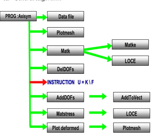
A. General Algorithm
PROG :Axisym Data file
Plotmesh
Matk
LOCE Matke
DelDOFs
AddDOFs AddToVect
Matstress LOCE
Plot deformed Plotmesh
INSTRUCTION U = K \ F
PROG :Axisym Data file
Plotmesh
Matk
LOCE Matke
DelDOFs
AddDOFs AddToVect
Matstress LOCE
Plot deformed Plotmesh
[image:3.595.47.292.550.767.2]INSTRUCTION U = K \ F
Fig.3. General Algorithm of the Axisym Program
The two elaborate programs (Axisym CAXI_L, and Axisym CAXI_K) relating to finite elements CAXI_L, CAXI_K, presented above are written with MATLAB language, each program consists of a principal function Axisym and subroutines.
B. Description of Axisym program Principal function Axisym
It calls the various subroutines or functions for different calculations of an axisymmetric structure, using the formulations described above for each element.
Data file
It is a file function where all the relative data with the problem are introduced:
Table of the nodes coordinates. Table of the elements connectivity Elements thickness
Elasticity modulus Poisson's ratio
Boundary conditions (numbers of the fixed degrees of freedom)
Applied loading vector
The MATLAB instruction: [data] = feval (str2func (Name of the data file); open the data file and allows the various subroutines or functions to read the relating data.
Plot mesh function
This function gives a graphic posting of the meshes, the coordinates and the numbering of the nodes, which allows, with the layout the seized structure, a visual checking of the data (coordinates table and connectivity).
Matk function
This function contains the process of assembling the element stiffness matrices Ke provides by the function matke. The do loop is done on the elements, by using the function LOCE; which provides the insertion of each element term in the global stiffness matrix.
LOCE Function
According the connectivity table; this function provides the localization table (numbers) of the degrees of freedom for each element.
Matke function
The element stiffness matrix can be evaluated by Matke function.
DelDOFs function
Instruction U = K\F
Once the boundary conditions are applied, it only remains to solve the discrete system. The solution in displacement (with the nodes) can be obtained with instruction MATLAB U = K \ F to solve the linear equations system (Cholesky method).
AddDOFs function
With this function, the degrees of freedom of the fixed nodes are added to the displacement vector; that is removed by the DelDOFs function. The do loop is made on the numbers of the degrees of freedom add by using the AddToVect function.
AddToVect function
This function provides the resulting displacement vector for each degree of freedom.
Matstress function
With this function, we can calculate the stresses, using the formulation presented for each element.
Plottedeformed function
Finally, with this function we can obtain the deformed shape of the structure.
V. NUMERICALAPPLICATIONS
The purpose of this section is the validation of the elaborated programs. Also the comparison of the results obtained with the presented elements and those given by ANSYS.
A. Circular Plate (without transverse shearing)
A circular plate is subjected to uniformly distributed load; its geometry and mechanical properties are presented on the fig.4.
Table I shows the results obtained with the Axisym programs for elements CAXI_L and CAXI_K and the analytical solution [10] without taking into account the assumption of transverse shearing(TS).
fZ
20
h=0.1 in ν = 0.3 E=107 lb/m2
fZ=1 lb/m2
Clamped
fZ
20
h=0.1 in ν = 0.3 E=107 lb/m2
fZ=1 lb/m2
Clamped
Fig.4. Circular plate subjected to uniformly distributed load
TABLEI:VALUE OF MAXIMUM DISPLACEMENT (IN)
Meshes Analy
Sol. [10]
Prog:CAXI_L Error Prog:CAXI_K Error
2 elements
0,17
0,2113 24,29% 0,1705 0,29%
4
elements 0,1759 3,47% 0,1700 0,00%
Comment
Both elements CAXI_L and CAXI_K converge towards the analytical solution in a monotonous way.
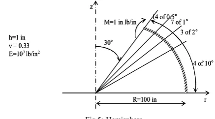
B. Hemisphere
A hemisphere shell structure (Fig.5) is modelled by truncated element CAXI_K (24 elements). The results obtained will be compared with the analytical solution [10], and with those given by ANSYS (Fig.6). All results are presented in Table II.
r z
30°
14 of 0.5° 7 of 1°
3 of 2°
4 of 10°
R=100 in M=1 in lb/in
h=1 in ν = 0.33 E=107 lb/in2
r z
30°
14 of 0.5° 7 of 1°
3 of 2°
4 of 10°
R=100 in M=1 in lb/in
h=1 in ν = 0.33 E=107 lb/in2
Fig.5:Hemisphere
TABLEII:VALUE OF MAXIMUM DISPLACEMENT (IN)
Mesh Analyt.
Sol. [10] ANSYS Prog:CAXI_K Error
24 elements 1,60E-05 1,59E-05 1,587E-05 0,81%
1
MN MX
X
Y
Z
-.159E-04-.137E-04 -.115E-04
-.928E-05 -.708E-05
-.487E-05 -.267E-05
-.464E-06 .174E-05
.395E-05
APR 1 2011 03:50:50 NODAL SOLUTION
STEP=1 SUB =1 TIME=1 /EXPANDED UX (AVG) RSYS=0 DMX =.318E-04 SMN =-.159E-04 SMX =.395E-05
U ROT M NFOR
NMOM
RFOR
RMOM
Fig. 6Deformed structure
Comment
The results obtained by the element CAXI_K are acceptable
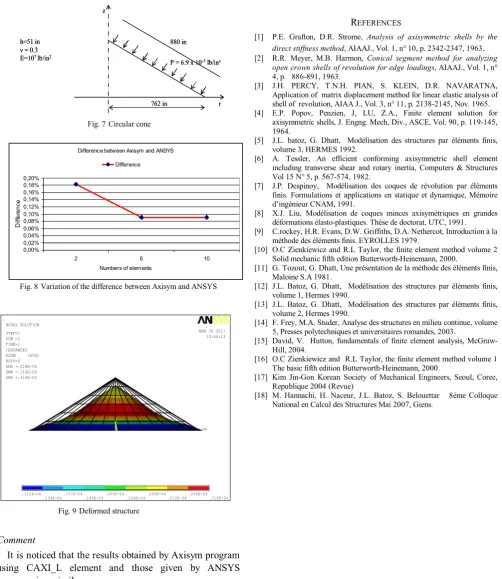
C. Circular cone
[image:4.595.319.538.217.338.2] [image:4.595.304.573.363.654.2]r z
762 in h=51 in
ν = 0.3 E=107 lb/in2
P = 6.9 x 10⁻³lb/in²
880 in
r z
762 in h=51 in
ν = 0.3 E=107 lb/in2
P = 6.9 x 10⁻³lb/in²
880 in
Fig. 7Circular cone
Difference between Axisym and ANSYS
0,00% 0,02% 0,04% 0,06% 0,08% 0,10% 0,12% 0,14% 0,16% 0,18% 0,20%
2 6 10
Numbers of elem ents
D
if
fe
ren
ce
Difference
Fig. 8Variation of the differencebetween Axisym and ANSYS
1
MN MX
X
Y
Z
.11 0E-04.134E-04 .157E-04
.180E-04 .203E-04
.226E-0 4 .249E-04
.272E-04 .295E-04
.318E-04 MAR 30 2011
10:44:13 NODAL SOLUTION
STEP=1 SUB =1 TIME=1 /EXPANDED USUM (AVG) RSYS=0 DMX =.318E-04 SMN =.110E-04 SMX =.318E-04
Fig. 9Deformed structure
Comment
It is noticed that the results obtained by Axisym program using CAXI_L element and those given by ANSYS converge in a similar way.
VI. CONCLUSION
From the results obtained above, the following conclusions can be drawn:
It can be observed that, the programs Axisym CAXI_L and CAXI_K give good results, which confirm the validation of the elaborated programs.
The presented CAXI_L and CAXI_K prove their efficiency in analysing axisymmetric shells structures.
REFERENCES
[1] P.E. Grafton, D.R. Strome, Analysis of axisymmetric shells by the direct stiffness method, AIAAJ., Vol. 1, n° 10, p. 2342-2347, 1963.
[2] R.R. Meyer, M.B. Harmon, Conical segment method for analyzing open crown shells of revolution for edge loadings, AIAAJ., Vol. 1, n° 4, p. 886-891, 1963.
[3] J.H. PERCY, T.N.H. PIAN, S. KLEIN, D.R. NAVARATNA, Application of matrix displacement method for linear elastic analysis of shell of revolution, AIAA J., Vol. 3, n° 11, p. 2138-2145, Nov. 1965. [4] E.P. Popov, Penzien, J, LU, Z.A., Finite element solution for
axisymmetric shells, J. Engng. Mech, Div., ASCE, Vol. 90, p. 119-145, 1964.
[5] J.L. batoz, G. Dhatt, Modélisation des structures par éléments finis, volume 3, HERMES 1992.
[6] A. Tessler, An efficient conforming axisymmetric shell element including transverse shear and rotary inertia, Computers & Structures Vol 15 N° 5, p. 567-574, 1982.
[7] J.P. Despinoy, Modélisation des coques de révolution par éléments finis. Formulations et applications en statique et dynamique, Mémoire d’ingénieur CNAM, 1991.
[8] X.J. Liu, Modélisation de coques minces axisymétriques en grandes déformations élasto-plastiques. Thèse de doctorat, UTC, 1991. [9] C.rockey, H.R. Evans, D.W. Griffiths, D.A. Nethercot, Introduction à la
méthode des éléments finis. EYROLLES 1979.
[10] O.C Zienkiewicz and R.L Taylor, the finite element method volume 2 Solid mechanic fifth edition Butterworth-Heinemann, 2000.
[11] G. Tozout, G. Dhatt, Une présentation de la méthode des éléments finis, Maloine S.A 1981.
[12] J.L. Batoz, G. Dhatt, Modélisation des structures par éléments finis, volume 1, Hermes 1990.
[13] J.L. Batoz, G. Dhatt, Modélisation des structures par éléments finis, volume 2, Hermes 1990.
[14] F. Frey, M.A. Studer, Analyse des structures en milieu continue, volume 5, Presses polytechniques et universitaires romandes, 2003.
[15] David, V. Hutton, fundamentals of finite element analysis, McGraw- Hill, 2004.
[16] O.C Zienkiewicz and R.L Taylor, the finite element method volume 1 The basic fifth edition Butterworth-Heinemann, 2000.
[17] Kim Jin-Gon Korean Society of Mechanical Engineers, Seoul, Coree, Republique 2004 (Revue)
[image:5.595.50.553.72.652.2] [image:5.595.52.283.384.578.2]