BME-HAS System for CoNLL–SIGMORPHON 2018 Shared Task:
Universal Morphological Reinflection
Judit ´Acs
Department of Automation and Applied Informatics Budapest University of Technology and Economics
and
Institute for Computer Science and Control Hungarian Academy of Sciences
Abstract
This paper presents an encoder-decoder neu-ral network based solution for both subtasks of the CoNLL–SIGMORPHON 2018 Shared Task: Universal Morphological Reinflection. All of our models are sequence-to-sequence neural networks with multiple encoders and a single decoder.
1 Introduction
Morphological inflection is the task of inflecting a lemma given either a target form or some con-textual information. Morphology has traditionally been solved by finite state transducers (FST) that employ a large number of handcrafted rules. The discrete nature of such processes makes it diffi-cult to directly translate transducers into neural networks and to effectively train them using back-propagation. There have been various attempts to replace parts of the FST paradigm with neural net-works (Aharoni and Goldberg,2016).
SIGMORPHON first organized a shared task on morphological inflection in 2016 (Cotterell et al.,
2016) which involved both inflection (inflect a word given its lemma) and reinflection (inflect a word given another inflected form of the same lemma). The winning solution (Kann and Sch¨utze,
2016) used a character sequence-to-sequence net-work with Bahdanau’s attention (Bahdanau et al.,
2015). In the second edition of the shared task (Cotterell et al.,2017) most teams used similar set-tings.
2 Task formulation
In this section we briefly describe the objective of the task and provide examples for each subtask. A more comprehensive explanation is available on the shared task’s website1 and in task description
paper (Cotterell et al.,2018).
1https://sigmorphon.github.io/sharedtasks/2018/
2.1 Task1: Type-level inflection
Inflection aims to find an inflected word given its lemma and a set of morphological tags in Uni-Morph MSD(Kirov et al.,2018). A few examples are shown below (the second column is the target):
release releasing V;V.PTCP;PRS
deodourize deodourize V;NFIN
outdance outdancing V;V.PTCP;PRS
misrepute misrepute V;NFIN
vanquish vanquished V;PST
resterilize resterilizes V;3;SG;PRS
The shared task features over 100 languages and 10 additional surprise language were released before the submission deadline. Most languages had three data settings: high (10 000 samples), medium (1 000 samples) and low (100 samples), except some low-resource languages that did not have enough samples for high or medium settings. Each language had a development set of 1 000 or less samples.
2.2 Task2: Inflection in context
Task2 is a cloze task. We were given a sentence with a number of missing word forms (usually 1 or 2) and our task is to inflect the word given its lemma and context. Task2 two had two tracks: in Track1 all the lemmas and morphosyntactic de-scription are given in the sentence context (the morphosyntactic description of the covered word is covered too), and in Track2 only the word forms of the context are given. Below are examples from Track1:
Les le DET;DEF;FEM;PL
compagnies compagnie N;FEM;PL
a´eriennes a´erien ADJ;FEM;PL
`
a `a ADP
bas bas ADJ;MASC;SG
coˆut coˆut N;MASC;SG
ne ne ADV;NEG
_ connaˆıtre _
pas pas ADV;NEG
la le DET;DEF;FEM;SG
crise crise N;FEM;SG
. . PUNCT
decoder
lemma encoder tag encoder
a l m a $ SOS N NOM PL $
lemma
attention attentiontag
lemma
context contextcontexttagtag
sigmoid output projection
tanh
[image:2.595.78.272.58.327.2]a
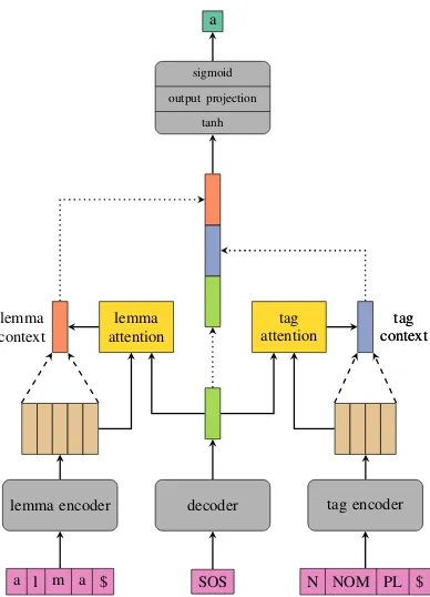
Figure 1: Two-headed attention model used for Task1. The figure illustrates the first timestep of decoding. The output of this step is fed back to the decoder in the next timestep. Modules are colored gray, attention heads yellow, inputs are purple, outputs are teal and en-coder output matrices are salmon. Dotted arrows rep-resent copy operations and dashed arrows reprep-resent at-tention summaries. The color scheme is borrowed from colorbrewer2.org
and the same sentence for Track2:
Les _ _
compagnies _ _
a´eriennes _ _
`
a _ _
bas _ _
coˆut _ _
ne _ _
_ connaˆıtre _
pas _ _
la _ _
crise _ _
. _ _
Both examples are taken from the development sets. The training sets have no covered words, and we generated training examples by covering a sin-gle word at a time, and using the rest as its sen-tence context.
Task2 also featured low, medium and high re-source settings with roughly 1 000, 10 000 and 100 000 tokens respectively.
3 Task1 model: two-headed attention
In this section we describe our system for Task 1: Type-level inflection. We explain our experimen-tal setup and the random hyperparameter search, and finally we list three slightly different submis-sions and their results.
3.1 Two-headed attention seq2seq
Inflection can be formulated as a mapping of two sequences, namely a lemma and a sequence of tags, to one sequence, the inflected word form. The lemma and the inflected word forms are char-acter sequences that usually share a common al-phabet while the tags are a sequence of language-specific morphological codes. Figure1illustrates our architecture. We use separate encoders for the lemma and the morphological tags and a sin-gle decoder. Both encoders employ character/tag embeddings and bidirectional LSTMs, where the outputs are summed over the two directions. The two encoders’ hidden states are then linearly pro-jected to the decoder’s hidden dimension and used to initialize the decoder’s hidden state. This allows using different hidden dimensions in each mod-ule. Decoding is done in an autoregressive fash-ion, one character at a time. At each timestep the decoder reads a single character: SOS (start-of-sequence)at first, the ground truth during training (teacher forcing) and the previous output during inference. The decoder uses a character level em-bedding, which may or may not be shared with the lemma encoder (c.f.3.2), then it passes the embed-ded symbol to a unidirectional LSTM. Its output is used by two attention modules, hence the name
two-headed attention, to compute a context vec-tor using Luong’s attention (Luong et al., 2015). The lemma and tag context vectors are concate-nated with the decoder output, then passed through atanh, an output projection and finally a sigmoid layer which produces a distribution over the char-acter vocabulary of the language. Greedy decod-ing is used.
3.2 Experimental setup
experi-ments. The framework is available on Github2and
the configurations and scripts used for this shared task are available in a separate repository3. The
latter repository contains all best configurations including the random seeds (we generate the ran-dom seeds at the beginning of each experiments, then save them for reproducibility).
All experiments shared a number of configura-tion opconfigura-tions while the others were randomly op-timized. We list the ones we fixed here and the others in3.3. Each experiment used a batch size of 128 for both training and evaluation except the ones on the Kurmanji language because the de-velopment dataset contained very long sequences and we had to reduce the batch size to 16 to fit into memory (12GB). We used the Adam opti-mizer with learning rate 0.001 and we stopped each experiment when the development loss did not decrease on average in the last 5 epochs com-pared to the previous 5 epochs. We ran at least 20 epochs before stopping even if the early stopping condition was satisfied to avoid early overfitting, which happened in about 10% of the experiments. We also set a hard upper limit for the number of epochs (200) but this was reached only two times out of 1 886 experiments. The average number of epochs before reaching the early stopping condi-tion was 51 and only 2.7% of experiments ran for more than 100 epochs. After each epoch, we saved the model if its development loss was lower than the previous minimum. We used cross entropy as the loss function.
3.3 Random parameter search
Our initial experiments suggested that the model is very sensitive to random initialization and the same configuration can result in models with very different performance. This is probably due to the limited training data even inhigh setting and the large number of parameters of the model. We chose three languages, Breton, Latin and Lithua-nian, and ran a large number of experiments with random configuration on them. The reason these were chosen is that the development accuracy on these were in the mid-ranges among all the lan-guage during our initial experiments. The follow-ing random experiments were all run on thehigh
training sets. Common parameters (c.f.3.2) were loaded from a base configuration and some
[image:3.595.306.526.80.274.2]param-2https://github.com/juditacs/deep-morphology 3https://github.com/juditacs/sigmorphon2018
Table 1: Parameter ranges
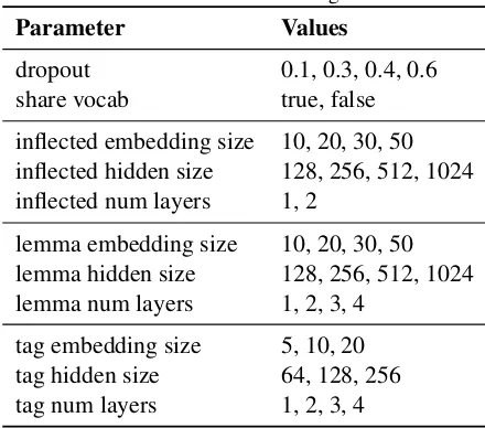
Parameter Values
dropout 0.1, 0.3, 0.4, 0.6 share vocab true, false inflected embedding size 10, 20, 30, 50 inflected hidden size 128, 256, 512, 1024 inflected num layers 1, 2
lemma embedding size 10, 20, 30, 50 lemma hidden size 128, 256, 512, 1024 lemma num layers 1, 2, 3, 4
tag embedding size 5, 10, 20 tag hidden size 64, 128, 256 tag num layers 1, 2, 3, 4
eters were overriden with a value uniformly sam-pled from a predefined set. The range of values are listed in Table1. Both encoders (lemma and tag) and the decoder (listed asinflected) have three varying parameters: the size of the embedding, the number of hidden LSTM cells and the num-ber of LSTM layers. We also varied the dropout rate for both the embedding and the LSTMs and the whether to share the vocabulary and the em-bedding among the lemma and the decoder or not. The running time of an experiment is dependent on the average length of the input sequences and the size of the vocabulary. It turns out that these vary greatly among the languages in the dataset. As listed in Table2 Breton is much ”smaller” in both alphabet and sequence length than Lithuanian or Latin and this was evident from the difference in average running time.
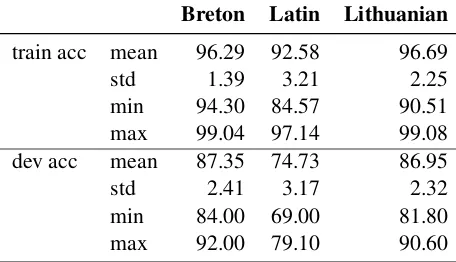
Table 3 summarizes the results of our random parameter search. Since the average running time of different language experiments is very differ-ent, we ended up running many more Breton ex-periments in roughly the same time. The standard deviation of results is quite large, especially for Breton, which we attribute to the small alphabet, the short sequences and the small number of lem-mas (44) as opposed to Latin (6517) or Lithuanian (1443).
pa-Table 2: Dataset statistics.
Breton Latin Lithuanian
alphabet size 27 55 58
inflected maxlen 14 23 32 inflected types 1790 9896 9463
lemma maxlen 11 19 28
lemma types 44 6517 1443
tag types 20 33 34
[image:4.595.77.513.81.230.2]tags maxlen 9 7 6
Table 3: Summary of the parameter search. The run-ning time is given in minutes.
Breton Latin Lithuanian
experiments 1033 610 243
dev acc meanmax 70.92 62.3293.00 78.90 80.2588.40 std 28.70 11.30 8.37
time mean 0.83 5.42 8.61
rameters can result in models with very different performance.
3.4 Submission
[image:4.595.72.297.251.344.2]We took the 5 highest scoring model for each lan-guage and trained a model with those parameters for each language and each data size, thus training 15 models per dataset. Our first submission is sim-ply the model with the highest development word accuracy. The second submission is the result of majority voting by all 15 models. The third one is the same as the first one but we changed the evalu-ation batch size from 128 to 16. This results fewer pad symbols on average. Table5 lists the mean performance of each submission.
Table 4: Accuracy statistics of 20 models trained with the same parameters but different random seed.
Breton Latin Lithuanian train acc mean 96.29 92.58 96.69
std 1.39 3.21 2.25
min 94.30 84.57 90.51 max 99.04 97.14 99.08 dev acc mean 87.35 74.73 86.95
std 2.41 3.17 2.32
min 84.00 69.00 81.80 max 92.00 79.10 90.60
Table 5: The mean accuracy of our Task1 submissions. Subm Data size Accuracy Ranking
#1 HighMedium 93.884884 767.430392 8 Low 3.742718 22
#2
High 94.662791 3
Medium 67.258824 10 Low 2.429126 25
#3 HighMedium 93.973256 667.357843 9 Low 3.634951 23
4 Task2: Inflection in Context
In this section we describe our system for Task2 - Track1, then explain how the model for Track2 differs from the model for Track1.
The development datasets for Task2 have two versions: covered and uncovered. An example is provided in2.2.
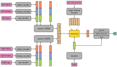
Figure 2 illustrates the model at a single timestep (decoding one character). The model has several inputs (colored purple):
target lemma The lemma of the target word. The inflected form of this lemma is the expected output.
left/right token context The other (inflected) to-kens in the sentence. Left context refers to the tokens preceding the covered token and right context refers to the ones succeeding it. left/right lemma context The lemmas of the
pre-ceding and succeeding tokens.
left/right tag context The corresponding tags of the preceding and succeeding tokens. previously decoded symbol Start-of-sequence at
the first timestep, then the last symbol pro-duced by greedy decoding.
[image:4.595.72.300.630.761.2]left tokeni
left lemmai
left tagsi
token encoder
lemma encoder
tag encoder
. . .
context LSTM
left
conte
xt
right tokeni
right lemmai
right tagsi
token encoder
lemma encoder
tag encoder
. . . context LSTM
right
conte
xt
decoder
SOS target lemma
encoder l e m m a
attention
sigmoid output projection
tanh
[image:5.595.75.525.59.316.2]a
Figure 2: Task2 architecture. The figure illustrates the first timestep of decoding. The output of this step is fed back to the decoder in the next timestep. The target lemma encoder’s hidden state is used to initialize the decoder hidden state (not pictured for the sake of clarity). The same coloring scheme is used as in1.
we acquire three fixed dimensional vector repre-sentation for each token. We concatenate these and use another biLSTM (context LSTM) to cre-ate a single vector representation of the left/right context. The context LSTM is shared by the left and the right context. The target lemma is en-coded by the same encoder as the other lemmas and inflected tokens and the output is used by the attention mechanism. The last hidden state of the encoder is used to initialize the hidden state of the decoder. Decoding is similar to the autoregressive process used in Task1 but there is only one atten-tion mechanism and it attends to the target lemma encoder outputs. Attention weights are computed using the concatenation of the decoder output at a single timestep and the left and right context vec-tors. The output of the attention module is con-catenated with the decoder output, passed through atanhand an output projection and finally a soft-max layer outputs a distribution over the character alphabet of the language. Similarly to our Task1 model, the ground truth is fed to the decoder at training time and the greedily decoded character at inference time. The cross entropy of the output distributions and the ground truth is used as a loss function.
Our model for Track2 is very similar to the model for Track1, except the left and right lemma
and tag encoders are missing and the context vec-tors are derived only from the left and right tokens.
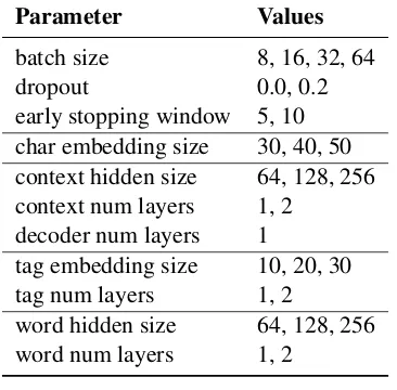
4.1 Experimental setup
Since our experiments for Task2 were significantly slower than the ones for Task1, we were unable to run extensive parameter search. We did perform a smaller version of the same random search using the parameter ranges listed in Table6. We chose the French dataset with medium setting, which is about 10 000 tokens. The average length of one experiment was 100 minutes and we were able to run 38 experiments. We ran the best configuration of the 38 on each language and each data size at least once. Since our parameter search was very limited, we also varied the parameters manually and tried other combinations. The exact configu-rations are available on the GitHub repository. All experiments were run on NVIDIA GTX TITAN X GPUs (12GB), since they did not fit into the mem-ory of the smaller cards (4GB).
Table 6: Predefined parameter ranges used for Task2 parameter search.
Parameter Values
batch size 8, 16, 32, 64
dropout 0.0, 0.2
early stopping window 5, 10 char embedding size 30, 40, 50 context hidden size 64, 128, 256 context num layers 1, 2
decoder num layers 1
tag embedding size 10, 20, 30 tag num layers 1, 2
word hidden size 64, 128, 256 word num layers 1, 2
Table 7: Task2 results.
Track1 Track2
high med low high med low
de 73.21 56.83 30.64 64.61 52.17 27.81 en 76.23 66.77 61.33 69.89 64.05 56.90 es 56.10 42.50 29.17 41.65 32.12 27.77 fi 53.75 22.11 10.29 30.24 17.15 8.89 fr 67.21 51.12 26.27 45.42 23.63 9.57 ru 67.67 38.76 21.59 56.73 33.73 19.68 sv 65.64 41.91 26.06 54.26 34.89 22.34
4.2 Submission and results
For both Track1 and Track2 we only submitted one system, the output of the highest scoring model on the development dataset. In both tracks, we finished in 2nd place. Table7lists our detailed results.
5 Conclusion
We presented our submissions for the CoNLL–SIGMORPHON 2018 Shared Task: Universal Morphological Reinflection. We em-ployed variations of sequence-to-sequence or encoder-decoder networks with Luong attention. Our experiments for Task1 suggest that at the current data size, the model is very sensitive to random initialization, so we used an ensemble of many systems, which placed 2nd of all teams in the high data setting. We also placed 2nd in both tracks of Task2. Our code and configuration files including the random seeds are available on Github.
References
Roee Aharoni and Yoav Goldberg. 2016. Morphologi-cal inflection generation with hard monotonic atten-tion. arXiv preprint arXiv:1611.01487.
Dzmitry Bahdanau, Kyunghyun Cho, and Yoshua Ben-gio. 2015. Neural machine translation by jointly learning to align and translate. InInternational Con-ference on Learning Representations (ICLR 2015).
Ryan Cotterell, Christo Kirov, John Sylak-Glassman, G´eraldine Walther, Ekaterina Vylomova, Arya D. McCarthy, Katharina Kann, Sebastian Mielke, Gar-rett Nicolai, Miikka Silfverberg, David Yarowsky, Jason Eisner, and Mans Hulden. 2018. The CoNLL– SIGMORPHON 2018 shared task: Universal mor-phological reinflection. In Proceedings of the CoNLL–SIGMORPHON 2018 Shared Task: Univer-sal Morphological Reinflection, Brussels, Belgium. Association for Computational Linguistics.
Ryan Cotterell, Christo Kirov, John Sylak-Glassman, G´eraldine Walther, Ekaterina Vylomova, Patrick Xia, Manaal Faruqui, Sandra K¨ubler, David Yarowsky, Jason Eisner, and Mans Hulden. 2017. The CoNLL-SIGMORPHON 2017 shared task: Universal morphological reinflection in 52 languages. In Proceedings of the CoNLL-SIGMORPHON 2017 Shared Task: Universal Mor-phological Reinflection, Vancouver, Canada. Asso-ciation for Computational Linguistics.
Ryan Cotterell, Christo Kirov, John Sylak-Glassman, David Yarowsky, Jason Eisner, and Mans Hulden. 2016. The SIGMORPHON 2016 shared task— morphological reinflection. In Proceedings of the 2016 Meeting of SIGMORPHON, Berlin, Germany. Association for Computational Linguistics.
Katharina Kann and Hinrich Sch¨utze. 2016. MED: The LMU system for the SIGMORPHON 2016 shared task on morphological reinflection. ACL 2016, page 62.
Christo Kirov, Ryan Cotterell, John Sylak-Glassman, G´eraldine Walther, Ekaterina Vylomova, Patrick Xia, Manaal Faruqui, Sebastian Mielke, Arya D. McCarthy, Sandra K¨ubler, David Yarowsky, Ja-son Eisner, and Mans Hulden. 2018. UniMorph 2.0: Universal Morphology. InProceedings of the Eleventh International Conference on Language Re-sources and Evaluation (LREC 2018), Miyazaki, Japan. European Language Resources Association (ELRA).