On the Construction of Separable-Variables
Conductivity Functions, and Their Application for
Approaching Numerical Solutions of the
Two-Dimensional Electrical Impedance Equation
M.P. Ramirez T., IAENG Member, M. C. Robles G., R. A. Hernandez-Becerril
Abstract—We analyze a technique for obtaining piecewise separable-variables conductivity functions, employing standard cubic polynomial interpolation. Our goal is to start making possible the practical use of the Pseudoanalytic Function Theory in medical imaging, by allowing the construction of numerical solutions, in terms of Taylor series in formal powers, of the two-dimensional Electrical Impedance Equation.
Keywords: Electrical Impedance Equation, pseudoanalytic func-tions
I. INTRODUCTION
The analysis of the two-dimensional Electrical Impedance Equation
∇ ·(σ∇u) = 0, (1)
is the departure point for any proper study of the Electrical Impedance Tomography problem.
As a matter of fact, we will find that the complexity of this governing equation, appears just at the very beginning, when the selection of the mathematical representation for the conductivityσ takes place.
There exists a wide collection of interesting methods for approaching the electric potentialuonce σhas been chosen. Many of them are based upon variations of the well known Finite Element Method (see e.g. [9]), which effectiveness has been well proved in many classes of boundary value problems belonging to the Electromagnetic Theory.
Still, most of the known variations of the Finite Element Method present instability when approaching solutions for the inverse problem of (1), and it is not clear yet how to overpass this situation.
An interesting alternative for solving (1) appeared when K. Astala and L. Païvarïnta [1] first noticed that the two-dimensional case of (1) was directly related with a special class of Vekua equation [11], and V. Kravchenko et al. [6] posed the structure of its general solution in analytic form by means of Taylor series in formal powers, employing elements of the Pseudoanalytic Function Theory developed by L. Bers [2].
We may also remark that the use of this new mathematical tools allowed to approach the solution of the direct boundary
Facultad de Ingenieria de la Universidad La Salle, A.C., B. Franklin 47, C.P. 06140, Mexico D.F., Mexico. email: [email protected]
The authors would like to acknowledge the support of CONACyT project 106722, Mexico.
value problem for (1), with high accuracy, once σwas posed as a separable-variables function [4].
These new results are, with no doubt, relevant for better understanding the dynamics of the Electrical Impedance Equa-tion. Thus, a natural path to follow, is to search for the interpolating methods that will allow us to apply these novel techniques, when studying cases situated nearer to the medical imaging engineering.
This work is dedicated to analyze one interpolating method posed in [7], that allows to obtain separable-variables functions
σ when a finite set of conductivity values is properly defined within a bounded domain.
Specifically, after reviewing a collection of statments cor-responding to the Pseudoanalytic Function Theory, we will discuss how to construct a piecewise polynomial separable-variables function by using standard interpolation methods.
Starting with the case used in [4], for approaching solutions of the boundary value problem for (1), we present the results of performing a basic numerical analysis, in order to test the convergence of the interpolation method. We illustrate the behavior of a certain class of maxima errors, taking into account the number of subregions in which we divided a unitary circle, and the number of points considered within every subregion.
We close with a brief discussion about the validity and use of these preliminary results, emphasizing the necessary work before we can use effectively this interpolation method in medical imaging.
II. PRELIMINARIES
Following [2], let the pair of complex-valued functions (F, G)fulfil the condition
Im F G
>0, (2)
where F denotes the complex conjugation of F. Thus any complex functionW can be expressed by means of the linear combination of F andG:
W =φF+ψG.
Here φ and ψ are real functions. A pair of functions satis-fying (2) is named a Bers generating pair. Indeed, L. Bers introduced a derivative based upon the generating pair(F, G). It has the form
where∂z=∂x∂ −i∂y∂ , andirepresents the standard imaginary
uniti2=−1. But this derivative will exist iff
(∂zφ)F+ (∂zψ)G= 0 (4)
holds, where ∂z = ∂x∂ +i∂y∂ (the reader should notice that
traditionally the differential operators∂zand∂zare introduced
with the factor12, but in our study it will result somehow more convenient to work without it). Introducing the notations
A(F,G)=
F ∂zG−G∂zF
F G−F G , B(F,G)=
F ∂zG−G∂zF
F G−F G , (5)
a(F,G)=
G∂zF−F ∂zG
F G−F G , b(F,G)=
F ∂zG−G∂zF
F G−F G ;
the equation (3) becomes
∂(F,G)W =∂zW −A(F,G)W−B(F,G)W , (6)
whereas (4) reaches
∂zW −a(F,G)W −b(F,G)W = 0. (7)
Specifically, the expressions (5) are called the characteristic coefficients of the generating pair (F, G); the relation (6) is referred as the derivative in the sense of Bers of W, or simply the(F, G)-derivative ofW; and (7) is in fact theVekua equation [11], which will play a central role in our further discussions.
We will define a complex valued function W fulfilling (7) as an (F, G)-pseudoanalytic function. The next statements were all originally posed in [2], and extended to the Applied Sciences in [5].
Definition 1: Let(F0, G0)and(F1, G1)be two generating pairs, and let their characteristic coefficients (5) satisfy the relations
a(F0,G0)=a(F1,G1),
B(F0,G0)=−b(F1,G1).
Then, (F1, G1) will be called a successor pair of (F0, G0), as well as (F0, G0) will be named the predecessor pair of (F1, G1).
Definition 2: Let the set of generating pairs {(Fn, Gn)},
n = 0,±1,±2, ... posses the following property: Every (Fn+1, Gn+1)is a successor of(Fn, Gn). The set{(Fn, Gn)}
is then called a generating sequence. If the generating pair (F, G) = (F0, G0), we say that (F , G) is embedded into {(Fn, Gn)}. Beside, if a number k exists such that
(Fn+k, Gn+k) = (Fn, Gn), the generating sequence is
classi-fied as periodic, with period equal tok.
Remark 1: Notice the (F0, G0)-derivative of an (F0, G0) -pseudoanalytic function will be(F1, G1)-pseudoanalytic. This implies if one is to know the m-derivative in the sense of Bers of an(F0, G0)-pseudoanalytic function, it is a requisite to posses in exact form all generating pairs, fromn= 0tilln=
m, belonging to the generating sequence in which(F0, G0)is embedded.
L. Bers also introduced the notion of an(F0, G0)-integral. We refer the reader to the specialized literature for examine the details of the existence of such integral [2], since in the current pages we will use exclusively(F0, G0)-integrable functions.
Definition 3: The adjoint generating pair (F0∗, G∗0) corre-sponding to(F0, G0)is introduced as
F0∗=− 2F0 F0G0−F0G0
, G∗= 2G0
F0G0−F0G0
.
Definition 4: When it exists, the (F0, G0)-integral of a complex valued function W is defined as
Z z
z0
W d(F0,G0)z=F0Re
Z z
z0
G∗0W dz+G0Re Z z
z0
F0∗W dz.
Particularly, the (F0, G0)-integral of the derivative in the sense of Bers of an (F0, G0)-pseudoanalytic function W:
∂(F0,G0)W, reaches
Z z
z0
∂(F0,G0)W d(F0,G0)z=W−φ(z0)F−ψ(z0)G,
and since the (F0, G0)-derivatives of (F0, G0) vanish identi-cally:
∂(F0,G0)F0≡∂(F0,G0)G0≡0,
the last integral expression represents the (F0, G0 )-antiderivative of the function ∂(F0,G0)W.
A. Formal powers
The classical Complex Analysis shows that any analytic function ϕ with respect to a complex variable z = x−iy:
∂zϕ= 0; can be expanded in Taylor series
ϕ=
∞
X
n=0
∂n zϕ(z0)
n! (z−z0)
n
,
where ∂zn = ∂z∂nn, z =x+iy and z0 is a fixed point in the plain, called the center of the series.
L. Bers generalized this classical result for the set of pseudoanalytic functions, employing what he called formal powers.
Definition 5: The formal powerZm(0)(a0, z0;z)with formal exponent0, complex constant coefficienta0, center at z0and depending upon z; is defined by the expression
Zm(0)(a0, z0;z) =λmFm+µmGm,
where
λmF(z0) +µmG(z0) =a0.
The formal powers with higher exponents are defined by the recursive formulas
Zm(n)(an, z0;z) =n Z z
z0
Zm−(n−11)(a0, z0;z)d(Fm,Gm)z.
Notice the integral operators are indeed antiderivatives in the sense of Bers.
In the light of the last statements, L. Bers proved that any (Fm, Gm)-pseudoanalytic function can be expressed by means
of Taylor series in formal powers:
W =
∞
X
n=0
Zm(n)(an, z0;z), (8)
where
an=
∂(nF
m,Gm)W(z0)
n! .
III. THE TWO-DIMENSIONALELECTRICALIMPEDANCE EQUATION
As it was mentioned before, K. Astala and L. Paï-varïnta proved in [1] the biunique relation between the two-dimensional (1) and a special Vekua equation, which was rediscovered and employed in a variety of works (see e.g. [5], [10]). This represents a very important advance since the study of the solutions for the direct problem of (1), is a critical matter when approaching solutions for its inverse problem, which is indeed the Electrical Impedance Tomography problem.
We should remark that positive results were obtained by assuming the electrical conductivity functionσas a separable-variables function
σ(x1, x2) =σ1(x1)σ2(x2).
More precisely, the example σ = ek1x1+k2x2 played the
main role in many works (see [4], [6]). Still, the majority of the novel results can apply when a wide class of different separable-variables function is considered.
Our proposal then, is to consider a piecewise separable-variables function, obtained by applying a polynomial inter-polation method to a set of conductivity values [7], that could have well been acquired from a medical image. In order to prove the validity of this suggestion, we will now briefly review the requirements that the interpolation method must fulfil, for working as part of the base on which the method of Taylor series in formal powers can be applied.
According to the notations of [10], by introducing the functions
W =−√σ ∂ ∂x1
u+i√σ ∂ ∂x2
u, (9)
∂z=
∂ ∂x1
+i ∂ ∂x2
,
p= p
σ2(x2) p
σ1(x1)
,
the two-dimensional Electrical Impedance Equation will turn into the Vekua equation
∂zW−
∂zp
p W = 0. (10)
The reader can verify that, for this case, a generating pair (F0, G0)is
F0=p, G0=ip−1,
and that this generating pair is embedded into a periodic generating sequence with period2 [2], [5], for which
Fm=
p
σ2(x2) p
σ1(x1)
,
Gm=i
p
σ1(x1) p
σ2(x2) ;
whenm is an even number, and
Fm=
p
σ1(x1)σ2(x2),
Gm=i
1 p
σ1(x1)σ2(x2) ;
when mis odd.
It becomes evident that once the piecewise interpolating polynomial function have approached a separable-variables conductivity function σ, the construction of the generating pairs (F0, G0) and (F1, G1) must be achieved by simple arithmetical operations.
It is easy to see that(F1, G1)can be obtained immediately, taking the squared root of σ. The main challenge lies on the construction of(F0, G0), since according to the notations (9), this pair should rise through the algebraic division of the function depending upon x2 over such depending uponx1.
Intending to give a positive answer to this question, we follow the method posed in [7] (also analized in [8]).
A. A piecewise separable-variable conductivity function
Let us consider a circular bounded domain with radius equal to 1, and let us separate such domain into a finite set of subregions created through the trace of parallel lines to the
x2-axis.
For simplicity, we will assume that the parallel lines have identical distance between them, and they are symmetrically distributed inside the circular domain.
After this sectioning procedure, we will observe q subre-gions created by the trace of q−1 parallel lines. Now trace a new set of parallel lines to the x2-axis, crossing precisely at the middle distance of the first set of lines. Select on every new parallel line a finite set of a points equally distributed on the line and inside the domain, assigning to every point a constant conductivity value.
We will have then a finite set of a×q conductivity values distributed across the parallel lines, each of them located on one subregion of the circle. Following the ideas posed in [7], the piecewise separable-variables function will have the form:
σ(x1, x2) =σ1(x1)σ2(x2) =
=
(x1+A)
(ξ1+A)f1(x2) ; 1≥x1>1−
2
q;
(x1+A)
(ξ2+A)f2(x2) ; 1−
2
q ≥x1>1−
4
q;
(x1+A)
(ξ3+A)f3(x2) ; 1−
4
q ≥x1>1−
6
q;
(x1+A)
(ξ4+A)f4(x2) ; 1−
6
q ≥x1>1−
8
q;
...
(x1+A)
(ξq+A)fq(x2) ;−1 + 2
q ≥x1≥ −1.
(11)
Here, ξ1, ξ2, ..., ξq represent the common x1 coordinate to every set of points located on the line crossing every subregion, andAis a real constant such thatx1+A6= 0within the circle. Other hand, every fk(x2), k = 1,2, ..., q are simply in-terpolating functions created by using standard cubic splines algorithms, each one corresponding to the collection of points selected on the parallel lines.
For simplicity, let us construct the piecewise function
p2=F02= σ(x2)
σ(x1)
,
according to the expression
F02= σ(x2)
=
(ξ1+A)
(x1+A)f1(x2) ; 1≥x1>1−
2
q;
(ξ2+A)
(x1+A)f2(x2) ; 1−
2
q ≥x1>1−
4
q;
(ξ3+A)
(x1+A)f3(x2) ; 1−
4
q ≥x1>1−6q;
(ξ4+A)
(x1+A)f4(x2) ; 1−
6
q ≥x1>1−
8
q;
...
(ξq+A)
(x1+A)fq(x2) ;−1 +
2
q ≥x1≥ −1.
(12)
B. Basic trials of convergence
A basic numerical analysis for the proposal is now in order. We will consider first the example of the conductivity function
F−21=σ=ek1x1+k2x2,
adopting k1 = k2 = 3, and A = 10. We will establish the maximum number of subregionsq= 100, and the maximum points on every line inside the circlea= 100.
We employ the criteria of locating the maximum erroremax
inside the region for everyqandacombination, according to the rule
emax=
q
(σo−σint)
2
,
where σo represents the original conductivity and σint the
piecewise interpolated function.
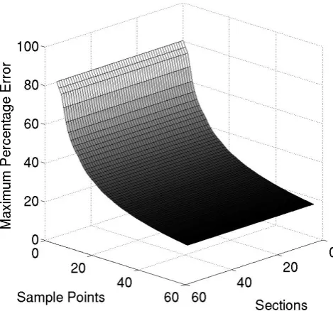
[image:4.595.310.544.235.449.2]Figure 1 displays the behavior of the maximum error, when sampling the interpolated functionσ at 99% of the limits of every region. We intend to be as close as possible of the places where the interpolating technique evidently has the biggest difference when compared to the original function.
Fig. 1. Example 1A
As expected, the maximum error does not decrease sig-nificantly when increasing a, due to the smoothness of the functione3x1+3x2, but it does when incrementing the number
of subregions q. Te computational procedure reported the minimum error emax atq=a= 100, being of1.2%.
Yet, by virtue of the graphical appreciation, we displayed the values corresponding to q= a= 60. Basically, they are not significant variations on the remaining values to be shown in the graphic. This restriction was also applied for the rest of the figures.
More interesting trial is the one performed considering
F02=e−3x1+3x2,
the function defined according to (12). Following the same steps, the minimumemaxwas registered atq=a= 100, being
of 1.9%. The behavior of the maximum error is illustrated in Figure 2.
Fig. 2. Example 1B
Trying to understand better the dynamics of the posed inter-polation technique, we performed a new experiment proposing
F−21=σ1(x1)σ2(x2) =
= (10 + sin (2πx2) + sin (4πx2) + sin (6πx2) + sin (8πx2))·
·(10 + cos (2πx2) + cos (4πx2) + cos (6πx2) + cos (8πx2)).
For this example we considered a maximum number of points
a = 200 and a maximum number of regions q = 200. The minimum error was located at the maxima of q anda, being 0.06%. Figure 3 shows the dynamics of the maximum error
emax.
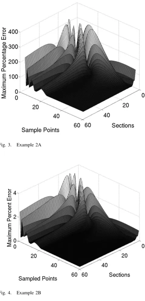
Finally, it was considered the case
F02=
σ2(x2)
σ1(x1)
,
and the interpolating function (12). Once more, we posed the maxima at q=a= 200. The minimum emax was located at
[image:4.595.45.280.449.668.2]Fig. 3. Example 2A
Fig. 4. Example 2B
IV. CONCLUSIONS
The possibility of applying the elements of Pseudoanalytic Function Theory to the Electrical Impedance Equation, con-sidering conductivity functions obtained from real medical images, is an interesting tool that opens the path for posing new and important questions.
We believe it is very important to remark in this last section some of the main areas to which we may direct our efforts, in order to make the novel rising theory of Electrical Impedance Tomography, fully applicable to practical cases.
In many senses, the results presented above are, indeed, preliminaries, since we have only considered conductivity functions which smoothness is well known, even the math-ematical expressions employed could suggest a higher degree
of complexity.
It is evident that the technique has to be tested when considering a wide range of geometrical figures with different classes of conductivities, within domains that does not share with the unitary circle. Beside, such tests must include strong changes in the values of the conductivity, through very small sections of the plane, as it would correspond to any clinical application.
Moreover, the very nature of the suggested interpolating function has indeed provoked the existence of discontinuities into the bounded domain, providing the precise condition for the uprising of anisotropic effects. A. P. Calderon did not consider such a case when he posed the Electrical Impedance Tomography problem, since the biunique correspondence be-tween a boundary electric potential function u and the elec-trical conductivity inside the domain can not be warranted anymore.
Of course, the case is very interesting, but overpasses the controlled conditions that may be established in order to better understand the dynamics of a problem that has been historically classified as very unstable. This implies the interpolating procedure posed before, should be modified to avoid this undesirable situation as soon as possible.
It is also important to remark that we have arbitrarily taken an equal number of points located at every line traced among the subregions. Evidently, this will not be convenient, even possible, when dealing with a wide class of medical images, very often required in clinical monitoring.
Taking into account this matters, the reader might consider this work as a basic proposal that intends to start a discussion in order to identify better techniques for the engineering work in medical instrumentation, based upon novel mathematical tools into the field of the Electrical Impedance Tomography.
REFERENCES
[1] K. Astala and L. Päivärinta,Calderón’s inverse conductivity problem in plane, Annals of Mathematics No. 163, 265-299, 2006.
[2] L. Bers,Theory of Pseudo-Analytic Functions,Institute of Mathematics and Mechanics, New York University, New York, 1953.
[3] A. P. Calderon, On an inverse boundary value problem, Seminar on Numerical Analysis and its Applications to Continuum Physics, Sociedade Brasileira de Matematica, pp. 65-73, 1980.
[4] R. Castillo P., V. V. Krvachenko, R. Reseniz V. ,Solution of boundary and eigenvalue problems for second-order elliptic operators in the plane using pseudoanalytic formal powers, Mathematical Methods in the Applied Sciences, Vol. 34, Issue 4, pp. 445-468, 2011.
[5] V. V. Kravchenko, Applied Pseudoanalytic Function Theory, Series: Frontiers in Mathematics, ISBN: 978-3-0346-0003-3, 2009.
[6] V. V. Kravchenko, H. Oviedo, On explicitly solvable Vekua equations and explicit solution of the stationary Schrödinger equation and of the equationdiv(σ∇u) = 0, Complex Variables and Elliptic Equations, Vol. 52, No. 5, pp. 353-366, 2007.
[7] M. P. Ramirez T.,On the electrical current distributions for the gener-alized Ohm’s Law, Submited for publication to Applied Mathematics and Computation, Elsevier, 2010. Avaliable in electronic format at http://www.arxiv.com
[8] M.P. Ramirez T., M. C. Robles G., R. A. Hernandez-Becerril, On a numerical interpolation technique for obtaining piecewise separable-variables conductivity functions, Proceedings of the 12th International Conference in Electrical Impedance Tomography, Bath, U.K., 2011 (accepted for publication).
[10] M. P. Ramirez T., V. D. Sanchez N., O. Rodriguez T., A. Gutierrez S., On the General Solution for the Two-Dimensional Electrical Impedance Equation in Terms of Taylor Series in Formal Powers, IAENG Interna-tional Journal of Applied Mathematics, 39:4, IJAM_39_4_13, Volume 39 Issue 4, ISSN: 1992-9986 (online version); 1992-9978 (print version), 2010.