Face Recognition using Common Vector based on
Curvelet Transform
Lifang Wei, Yanfeng Sun, Baocai Yin
Abstract—In this paper, a novel approach for expression invariant face recognition is proposed. It's implemented by common vector and the feature extraction is based on Curvelet transform, which is one of the multiscale geometric transforms and has better sparsity than the other transforms, especially for the edges. We assume the different images of the same subject as an interrelated ensemble with expression variations which could be viewed as sparse respectively. Then, each subject can be represented by a common feature vector, capturing its essential features, and an innovation feature vector, corresponding to the expression variations. By keeping the two feature vectors of each subject, we can use them to classify an image by the minimum reconstruction error.
Index Terms—Face recognition, Curvelet transform, common feature vector, innovation feature vector
esearch on face recognition has shown great maturity as developing for several decades. And many quite efficient approaches have emerged. Approaches based on linear subspace, such as PCA[1], LDA[2] and ICA[3] are commonly used. Although they have the capability to achieve rather good results for recognition, there still exist some limitations. For PCA and LDA, they have advantages in representing facial images, but involve in a high interrelation among the samples and being not robust for facial images with expression variations. Moreover, LDA is usually followed by the singularity problem. ICA overcomes these defects, but it's more complex than PCA and LDA.
To solve the limitations of linear subspace approaches, especially for singularity problem resulting from limited sample images, the Common Vector method [4][5] was proposed. It extracted essential common features from the same subject by discarding their differences. The Discriminative Common Vector based on linear subspace
Manuscript received December 6, 2010. This paper is supported by the National Natural Science Foundation of China (No. 60973057, 60825203, 61070117).
Lifang Wei is with Beijing Key Laboratory of Multimedia and Intelligent Software Technology , College Of Computer Science and Technology , Beijing University Of Technology , Beijing. 100124, China (phone: 67396568-2310; emails:[email protected]).
Yanfeng Sun is with Beijing Key Laboratory of Multimedia and Intelligent Software Technology , College Of Computer Science and Technology , Beijing University Of Technology , Beijing. 100124, China (emails:[email protected]).
Baocai Yin is with Beijing Key Laboratory of Multimedia and Intelligent Software Technology , College Of Computer Science and Technology , Beijing University Of Technology , Beijing. 100124, China (emails: [email protected]).
and Gram-Schmidt orthogonalization is one of such methods. Then Pradeep and Baoxin Li proposed another common vector method—BJSM [6] based on Joint Sparsity Models. It combined DCT and compressive sensing theory to get the common feature vector and the innovation feature vector corresponding to expression variations of the same subject. BJSM not only reduced the storage spaces for training samples, but also improved the recognition rate of facial images with expression variations. Nevertheless, there still exists some space to improve it by extracting sparser representations of images. So we try to choose other advanced image transforms. The multiscale geometric transforms should give a high priority, which could explore rather sparser representations than DCT, and achieve a better recognition rate.
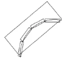
In 1999 Candes proposed a new multiscale geometric transform—Curvelet transform [8][9][10].Because of its high anisotropy and multi-orientations, Curvelet transform has provided rather optimal sparse representations of images, especially for the edges with competent handling of curve singularities. This sparse property profits from using oblong support for sparse approximation, unlike the wavelet transform which approximates curves in the way of point and keeps a great many coefficients.Figure1 demonstrates sparse approximation of Curvelet transform. Usually, facial images have variations in contour and the five sense organs (open or/close eyes, mouth). Moreover, capturing such information can be essentially helpful for face recognition with expression variations. That's why Curvelet transform gradually become popular in face recognition.
The method we proposed is a common vector method based on Curvelet transform and aims for improving face recognition with great expression variations. We extract each subject's common feature vector and innovation feature vector with the former containing the essential features and the latter containing expression variations related to all the images of the same subject. Firstly, we apply Curvelet transform to each training image and obtain coefficients in different scales and orientations. Then, we view the
I.INTRODUCTION
[image:1.595.359.463.553.653.2]R
transformed images of the same subject at each scale and orientation as a small ensemble. Then, using a formula based on the compressive sensing theory to compute the common component and innovation component of the same subject at each scale and orientation. Finally, merge these common components and innovation components to be as the subject's common feature vector and innovation feature vector. The common feature vectors and innovation vectors of all the subjects compose the common feature set and innovation feature set. Then we can test an image using the two sets.
Section 2 gives a brief introduction of Curvelet Transform. Section 3 presents our proposed method including Curvelet composition, feature extraction and classification. Section 4 displays the experimental results and analysis, and conclusion and future work in Section 5.
II.CURVELET TRANSFORM
Curvelet transform as one of multiscale geometric transforms has provided an essentially optimal representation of objects with discontinuous edges. At present, it has developed for two generations. The first generation Curvelet transform is essentially derived from ridgelet. To some extent, it can be defined as a transform based on ridgelet theory and subband filter theory. And the
Curvelet decomposition can be stated in four stages, including subband decomposition, smooth
partitioning, renormalization and ridgelet analysis. The main idea of the first generation curvelet transform in solving curve singularities is that curve can be viewed as line at rather small scales and then curve singularities are handled by line singularities.
Because of the complexity of the digital implementation for the first generation Curvelet transform, the second generation Curvelet transform was proposed. The second generation has no relation to the ridgelet theory, completely different from the first generation. As wavelet and ridgelet transforms, Curvelet transform also belongs to sparse theory category and continuous Curvelet can be represented as inner product of signal and base functions:
c
(
j
,
l
,
k
)
:
f
,
j,l,k (1)where
j,l,k is Curvelet. Respectively, j, l and k represent scale, direction and position. By defining two windows called "radial window" and "angular window "at scale j, we can create a window function using Parabolic scaling, with wedge support areas refined by "radial window" and "angular window". From figure 2 we can see that the wedge support areas contains all scales and orientations, which ensures the Curvelet transform being anisotropic. The representation of the window function in frequency domain is just the Curvelet at scale j. Since the Curvelet at scale j is known, the Curvelet at scale2
jcan be obtained through rotation and translation.
The second generation Curvelet transform has two digital implementations. One is Digital Curvelet Transform via Unequispaced FFTs, and the other is Digital Curvelet
Transform via Wrapping. In this paper, we choose the first one to use.
III.THE PROPOSED METHOD
Our proposed method aims to extraction common feature vector and innovation feature vector from images of the same subject in the Curvelet transform domain. The Curvelet decomposes at different scales and orientations. That means there will be several layers of decomposition coefficients. To get sparser and more accurate common feature and innovation feature, we extract common components and innovation components from each scale and orientation layer and then combine them to be as common feature vector and innovation feature vector of each subject.
A.Curvelet Decomposition
Through the second generation Curvelet transform, the facial image is decomposed of low frequency coefficients and high frequency coefficients. For a size
M
N
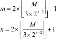
image, its decomposition scale s is determined bys[lb(min(M,N))3] (2)
where lb is log based binary. In addition, the decomposition scale s should neither be too large nor too small. Too large scale may result in losing some useful information. And too small scale performs low compression and retains great redundancy information. The first scale layer is coarse scale layer and the last is fine scale layer each with only one coefficients matrix because of having no directions. The size of the coarse coefficients matrix is determined by
1
2
3
2
1
2
3
2
2 2
s s
M
n
M
m
(3)
The size of the fine coefficients matrix is the same as the original image. The other scales are detailed scales and have multi-orientations at each scale. The number of orientations is usually multiple of 8.
[image:2.595.369.457.87.159.2]The coarse-scale layer contains all the low frequency coefficients capturing the essential part of an image. The detailed layer and fine layer coefficients are high frequency coefficients, which contains an image's edges and detailed information. Figure 3 shows each single layer's reconstructed image with the original image size256256. Since the coarse layer coefficients contain the essential information of an image, many authors used only the coarse layer for recognition and achieved expected results.
Fig. 2. The wedge support of Curvelet
[image:2.595.383.481.553.620.2]B. Feature Extraction
Although using only the coarse layer has achieved good results, it has not enough information for expression facial images with many edges and details, because the detailed layer and fine layer are also indispensable parts for recognition. Therefore, we will extract features from all the layers to achieve better recognition results.
Suppose there are C classes, each class with S images and
C k S N 1(k=1, 2, ... , C) . For size 64x64 original image, it
decomposes to three layers, coarse layer, detailed layers and fine layer. The coarse layer and the fine layer have only one coefficient matrix with size 32x32 and 64x64. And the detailed layers has 32 (4 big orientations, each with 8 small orientations) coefficient matrixes. Since we view each class as a big ensemble and each class images' same coefficient matrixes as a small ensemble, we should extract common components and innovation components from the 34 coefficient matrixes to get the common feature vector and the innovation feature vector. Following we introduce how to compute such a small ensemble's common components and innovation components.
For a size
m
n
coefficient matrix, all the same coefficient matrixes of the kth class images can be viewed as a small ensemble{
z
,}
R
mxn(
j
1
,
2
,
,
S
)
j
k
:
C
k
z
z
z
z
k k k kS,...,
2
,
1
],
[
,1 ,2 ,
(4)
For each
z
k,j, it can be partitioned into two separate parts: a common part ck
w
and a innovation part i j kw
, , namely,n m i j k c k i j k T c k T i j k c k j k
R
w
w
w
E
w
E
w
w
z
, , , ,,
,
(5)]
[
,1 i,S k i k c k
k
w
w
w
W
(6)From formula (4)-(6), we can write,
z
k
W
k , (7) where
1 2
,m mS T T T T
R
E
E
E
( )1
[
]
,m m
R
E
isan identity matrix , 2
(
1)
(mS) (mS)R
diag
.
1and
2 correspond to the common part and innovation part. ComputingW
k is equivalent to solve the following problem, k k k kW
z
t
s
W
W
.
.
min
arg
1 (8)Calculate
W
k by using GPSR(Gradient Projection for Sparse Reconstruction) algorithm .Then we can get matrixes ck
w
and ( )1 ,
S j i j k i k ik w w
w corresponding to the
common component and the innovation component.
In the above way, compute the common components and innovation components of the 34 coefficient matrixes from the coarse layer, detailed layers and fine layer in the kth class. The common feature vector and innovation feature vector of the kth class consist of these common components and innovation components. Due to the large amount of coefficients, it is necessary to find a way to compress them. For the coarse layer containing essential information, we reduce its common component and innovation component to a low dimension. However, the common components and innovation components of the detailed layers and fine layer are compressed by choosing only part of its coefficients for not all of them are necessary for recognition. Some have strong discrimination powers while others have very weak discrimination powers perhaps resulting from illumination and noise. Now our task is to find out the coefficients with great discrimination powers. We use a value to represent a coefficient's discrimination power called discriminant value. The greater the value is, the stronger the power is. On the contrary, the power is weak when the value is small. Here we use DPA (Discrimination Power Analysis) algorithm [12]to calculate the discriminant value.
For a coefficient matrix mn
R
X
,
mn m m n nx
x
x
x
x
x
x
x
x
X
2 1 3 22 21 1 12 11 (9)Since there are
C
S
training images, the discriminatevalue of each coefficient
)
,...,
2
,
1
;
,...,
2
,
1
(
i
m
j
n
x
ij
is computed as follows:(1)Construct matrix
A
ij: ) , ( ) 2 , ( ) 1 , ( ) , 2 ( ) 2 , 2 ( ) 1 , 2 ( ) , 1 ( ) 2 , 1 ( ) 1 , 1 ( C S x S x S x C x x x C x x x A ij ij ij ij ij ij ij ij ij ij (10)
(2)Compute the mean value and covariance of each class:
C c c s A S M S s ij c
ij ( , ), 1,2,...,
1 1
(11) C c M c s A V S s c ij ij cij ( ( , ) ) , 1,2,...,
1 2
(12)(3)The average of covariance of all the classes:
C c c ij W ijV
C
V
11
(13)(4)Compute the mean value and covariance of all the training samples:
1 ( , )
1 1 c s A C S M C c S s ij ij
(14)
2 1 1 ) ) , ( ( ij C c S s ij B
ij A s c M
V
(15)
(5)Compute the discriminant value at position (i,j):
N
j
M
i
V
V
j
i
D
W ij Bij
,
1
,
1
)
,
(
(16)(6)Construct matrix D:
mn m m m mD
D
D
D
D
D
D
D
D
D
2 1 2 22 21 1 12 11 (17)D is the discriminant value matrix corresponding to coefficient matrix X.
In the same way, using DPA compute the discriminant value of the 33 coefficient matrixes of the detailed and fine layers belonging to the kth class and single out the coefficients corresponding to the large values to compose the common feature vector and innovation feature vector. For each of the detailed common components and innovation components, we choose n2 coefficients with strong discrimination power. And n3 coefficients from the fine common component and fine innovation component. And we compress the coarse common component and innovation component to a n1 dimensions vector for reducing computation complexity. Finally, we get a (n1+32n2+n3) dimensions common feature vector and a (n1+32n2+n3) dimensions innovation feature vector for the kth class. Compute the other classes by the same way, we
can get a common feature vector set{Vc}(j 1,2,...,C)
j and a innovation feature vector set
{
i}
j
V
, c represents common and i represents innovation. Just keeping the two sets we can conduct classification and recognition.C. Classification
To decide which class the test image belongs to, we choose the minimum reconstruction error method for classification, with the common feature vector set and innovation feature vector set. Firstly, we apply the Curvelet transform to the test image and get the coarse coefficients, detailed coefficients and fine coefficients. For the coarse efficient matrix, compress it to a n1 dimensions vector. Then using DPA to single out n2 coefficients from each detailed coefficient matrix and n3 from the fine coefficient matrix. Therefore, we get a (n1+32n2+n3) dimensions feature vector t
V
for the test image. Reconstruct tV
by the common feature vector and innovation feature vector of each class.Assume the test image belongs to the jth class, t
V
can be represents by, ) ,..., 2 , 1 (, j C
r V
Vt jc ji (18)
where i j
r
is the innovation feature vector of the test image related to the jth class. Furthermore, extract a common componentf
jbetween ij
r
and ij
V
by formula (7).Then the reconstructed t
V
displays as:c j j t
f
V
V
ˆ
(19)Then, reconstruct t
V
by each class of the training set, and compute their reconstruction errors by,||) ˆ
(|| min
arg t t
k V V
(20)Eventually, the test image is classified to the kth class with the minimum reconstruction error.
IV.EXPERIMENTAL RESULTS AND ANALYSIS
We chose 3 facial expression databases for experiment: (1)JAFFE (Japanese Female facial expression database); (2)CMU-AMP facial expression database; (3) Yale facial expression database. We select 200 images from JAFFE database, 20 images for each person. Select J=2,3,4,5 images for each person and conduct experiments with 10 trials for each J. The CMU-AMP database contains 975 images, 75 images for each person. Set J=4,5,...,8 images for each person with 5 trials for each J. The Yale database contains 165 images, 15 images for each person. Set J=3,4,5 images for each person with 5 trials for each J. All the images from the three facial expression database are cropped to size 64x64.The common feature vector and innovation feature vector are set at respectively 486
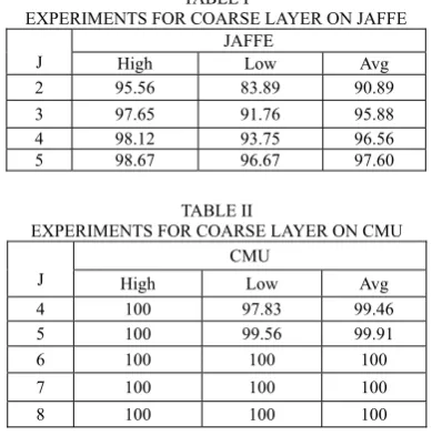
dimensions (n1=64,n2=12,n3=10), 480 dimensions (n1=150, n2=10,n3=10) and 730 dimensions (n1=400, n2=10, n3=10) corresponding to JAFFE, CMU-AMP and Yale databases. To prove the validation of Curvelet transform for face recognition, firstly, just use the coarse coefficients for experiments. From Table I and II, we can see the recognition rates are growing with the increasing number of the training images, with the highest rates 98.67% and 100% on JAFFE database and CMU database.
Although taking the coarse coefficients only for face recognition functions effectively, our proposed method can obtain better recognition results by adding the detailed coefficients and fine coefficients. These coefficients contain the edge and contour information of images which are especially important for recognition of the facial expression images. we performed experiments on two types of test sets. One is that involves the same facial expression images as the training set, the other is that doesn't involve any same expression images as the training set. JAFFE and CMU-AMP databases belongs to the first type, and Yale database goes to the second type. Here we compare our method with the BJSM method. From Table III, we can see that our proposed method's highest recognition rate reaches 100% while BJSM is 98.67% on JAFFE database. On CMU-AMP database, both the proposed method and BJSM method have achieved good results with highest recognition rate 100%, but our method is still better at J=4,5. For the Yale database, the whole experimental results are lower than the two other databases because of no same facial expression images between the test sets and the training sets. However, compared to BJSM, the highest recognition rates and the average rates have increased by about 2%.
V.CONCLUSION AND FUTURE WORK
We proposed a new method using common vector based on Curvelet transform for the expression invariant face recognition. By extracting the common feature vector and the innovation feature vector of the same subject in the Curvelet transform domain, we can only conserve the two feature vectors for recognition, while the original training samples take a lot of space, especially for quite a large face database. The two feature vectors are extracted from the common components and innovation components of all the coefficient layers of the same subject. Here, we choose DPA to compress the large amount of high frequency coefficients. In fact, there may exist many other better ways instead of DPA for coefficient selection. Apart from that, Curvelet Transform is not the most optimal image transform, so we can also replace it by other transforms with much better sparsity.
ACKNOWLEDGMENT
I would like to take this chance to express my sincere gratitude to my supervisors, Yanfeng Sun and Baocai Yin, who are professors of Beijing University Of Technology, for their
kindly assistance and valuable suggestions during the process of my thesis writing. My gratitude also extends to all the teachers who taught me during my graduate years for their kind encouragement and patient instructions. Last, I would like to offer my particular thanks to my friends and family, for their encouragement and support for the completion of this thesis.
REFERENCES
[1] Matthew A. Turk and Alex P. Pentland Face Recognition Using Eigenfaces. IEEE Conference on Computer Vision and Pattern Recognition,1991,586-591
[2] Peter N. Belhumeur,João P. Hespanha,and David J. Kriegman Eigenfaces vs. Fisherfaces:Recognition Using Class Specific Linear Projection. IEEE Transactions on Pattern Analysis and Machine Intelligence, 1997, 19(7): 711-720
[3] Jian Yang. Kernel ICA: An alternative formulation and its application to face recognition. Pattern Recognition. 2009,38(10): 1784-1787
[4] Gulmezoglu M.B.,Dzhafarov V.,Keskin M.,and Barkana A.,A Novel Approach to Isolated Word Recognition,IEEE Transactions Speech TABLE І
EXPERIMENTS FOR COARSE LAYER ON JAFFE J
JAFFE
High Low Avg 2 95.56 83.89 90.89 3 97.65 91.76 95.88 4 98.12 93.75 96.56 5 98.67 96.67 97.60
TABLE II
EXPERIMENTS FOR COARSE LAYER ON CMU J
CMU
High Low Avg 4 100 97.83 99.46 5 100 99.56 99.91 6 100 100 100 7 100 100 100 8 100 100 100
TABLE III
COMPARISON BETWEEN TWO ALGORITHM ON JAFFE JAFFE
J
Proposed Algorithm BJSM Algorithm
High Low Avg High Low Avg 2 97.22 86.11 92.84 95.56 83.89 90.94 3 98.82 94.12 96.71 97.65 91.76 95.88 4 99.38 95.63 96.94 98.12 93.75 96.62 5 100 96.67 98.53 98.67 96.67 97.80
TABLE IV
COMPARISON BETWEEN TWO ALGORITHM ON CMU CMU
J
Proposed Algorithm BJSM Algorithm
High Low Avg High Low Avg 4 100 99.46 99.83 100 97.94 99.50 5 100 100 100 100 99.67 99.93 6 100 100 100 100 100 100 7 100 100 100 100 100 100 8 100 100 100 100 100 100
TABLE V
COMPARISON BETWEEN TWO ALGORITHM ON YALE Yale
J
Proposed Algorithm BJSM Algorithm
[image:5.595.76.271.179.376.2]and Audio Processing,1999,7(6)
[5] Gulmezoglu M.B.,Dzhafarov V.,Keskin M.,and Barkana A.,The Common Vector Approach and Its Relation to Principal Component Analysis,IEEE Transactions Speech and Audio Processing,2001,9(6) [6] Pradeep Nagesh and Baoxin Li. A Compressive Sensing Approach
for Expression-Invariant Face Recognition. IEEE,2009
[7] Chelali F.Z. Face recognition system based on DCT and Neural Network. International Conference on Artificial Intelligence and Pattern Recognition, 2010:13-18
[8] Candes E J, Demanet L, Donoho D L. Fast discrete Curvelet transforms[R]. Applied and Computational Mathematics. California Institute of Technology,2005: 1-43.
[9] Candes E J, Donoho D L. New tight frames of Curvelets and optimal representations of objects with C2 singularities [J]. Communications on Pure and Applied mathematics, 2004, 57(2): 219-266.
[10] Candés E, Donoho D L. Curvelets-a surprisingly effective nonadaptive representation for objects with edges, Technical Report, Department of Statistics,Stanford University, USA, 1999
[11] Donoho D L. Compressed sensing. IEEE Transactions on Information Theory, 2006,52(4):1289-1306
[12] Saeed Dabbaghchian. Feature extraction using discrete cosine transform and discrimination power analysis with a face recognition technology. Pattern Recongniton. 2010, 43(4):1431-1440