and Lexical Language Model
Ming Tan
∗Wright State University
Wenli Zhou
∗∗Wright State University
Lei Zheng
†Wright State University
Shaojun Wang
‡ Wright State UniversityThis paper presents an attempt at building a large scale distributed composite language model that is formed by seamlessly integrating an n-gram model, a structured language model, and probabilistic latent semantic analysis under a directed Markov random field paradigm to simul-taneously account for local word lexical information, mid-range sentence syntactic structure, and long-span document semantic content. The composite language model has been trained by performing a convergent N-best list approximate EM algorithm and a follow-up EM algorithm to improve word prediction power on corpora with up to a billion tokens and stored on a supercomputer. The large scale distributed composite language model gives drastic perplexity reduction over n-grams and achieves significantly better translation quality measured by the Bleu score and “readability” of translations when applied to the task of re-ranking the N-best list from a state-of-the-art parsing-based machine translation system.
No rights reserved. This work was authored as part of the Contributor’s official duties as an Employee of
1. Introduction
The Markov chain (n-gram) source models, which predict each word on the basis of the previousn−1 words, have been the workhorses of state-of-the-art speech recognizers and machine translators that help to resolve acoustic or foreign language ambiguities by placing higher probability on more likely original underlying word strings. Although the Markov chains are efficient at encoding local word interactions, then-gram model
∗ Kno.e.sis Center and Department of Computer Science and Engineering, Wright State University, Dayton OH 45435. E-mail:[email protected].
∗∗ Kno.e.sis Center and Department of Computer Science and Engineering, Wright State University, Dayton OH 45435. E-mail:[email protected].
† Kno.e.sis Center, Wright State University, Dayton OH 45435. E-mail:[email protected].
‡ Kno.e.sis Center and Department of Computer Science and Engineering, Wright State University, Dayton OH 45435. E-mail:[email protected].
clearly ignores the rich syntactic and semantic structures that constrain natural lan-guages. Attempting to increase the order of ann-gram to capture longer range depen-dencies in natural language immediately runs into the curse of dimensionality (Bengio et al. 2003). The performance of conventionaln-gram technology has essentially reached a plateau (Rosenfeld 2000b; Zhang 2008), and it has proven remarkably difficult to improve onn-grams (Jelinek 1991; Jelinek and Chelba 1999). Research groups (Och 2005; Zhang, Hildebrand, and Vogel 2006; Brants et al. 2007; Emami, Papineni, and Sorensen 2007) have shown that using an immense distributed computing paradigm, up to 6-grams, can be trained on up to billions and trillions of tokens, yielding consistent sys-tem improvements because of excellentn-gram hit ratios on unseen test data, but Zhang (2008) did not observe much improvement beyond 6-grams. As the machine translation (MT) working groups stated in their final report (Lavie et al. 2006, page 3), “These approaches have resulted in small improvements in MT quality, but have not funda-mentally solved the problem. There is a dire need for developing novel approaches to language modeling.”
Over the past two decades, more sophisticated models have been developed that outperformn-grams; these are mainly the syntactic language models (Della Pietra et al. 1994; Chelba 2000; Chelba and Jelinek 2000; Charniak 2001; Roark 2001; Wang and Harper 2002; Jelinek 2004; Bened´ı and S ´anchez 2005; Van Uytsel and Compernolle 2005) that effectively exploit sentence-level syntactic structure of natural language, and the topic language models (Saul and Pereira 1997; Gildea and Hofmann 1999; Bellegarda 2000; Wallach 2006) that exploit document-level semantic content. Unfortunately, each of these language models only targets some specific, distinct linguistic phenomena (Pereira 2000; Rosenfeld 2000a, 2000b); thus, each captures and exploits different aspects of natural language regularity. A natural question we should ask is whether/how we can construct more complex and powerful but computationally tractable language models by integrating many existing/emerging language model components, with each component focusing on specific linguistic phenomena like syntactic structure, semantic topic, morphology, and pragmatics in complementary, supplementary, and coherent ways (Bellegarda 2001, 2003).
information in natural language, such as syntactic structure and semantic topic. The second weakness is that if the statistical model is too complex it becomes intractable to estimate model parameters; computationally very expensive Markov chain Monte Carlo sampling methods (Mark, Miller, and Grenander 1996; Rosenfeld 2000b; Rosenfeld, Chen, and Zhu 2001) would have to be used. One way to overcome the first hurdle is to use a preprocessing tool to extract hidden features (e.g., Rosenfeld [1996] used mutual information clustering method to find word pair triggers) then combine these triggers with trigrams through a maximum conditional entropy approach to allow the discourse topic to influence word prediction; Khudanpur and Wu (2000) used Chelba and Jelinek’s structured language model and a word clustering model to extract relevant grammatical and semantic features, then to again combine these features with trigrams through a maximum conditional entropy approach to form a syntactic, semantic, and lexical language model. Wang and colleagues (Wang et al. 2005a; Wang, Schuurmans, and Zhao 2012) have proposed thelatent maximum entropy (LME) principle, which extends standard maximum entropy estimation by incorporating hidden dependency structure, but still the LME wouldn’t overcome the second hurdle. The third method is
directed Markov random field(Wang et al. 2005b) that overcomes both weaknesses in the maximum entropy approach. Wang et al. used this approach to combine trigram, probabilistic context-free grammar (PCFG), and probabilistic latent semantic analysis (PLSA) models; a generalized inside–outside algorithm is derived that alters the well-known inside–outside algorithm for PCFG (Baker 1979; Lari and Young 1990) with modular modification to take into account the effect ofn-gram and PLSA while remain-ing at the same cubic time complexity. When applyremain-ing this to the Wall Street Journal corpus with 40 million tokens, they achieved moderate perplexity reduction. Because the probabilistic dependency structure in a structured language model (SLM) (Chelba 2000; Chelba and Jelinek 2000) is more complex and powerful than that in a PCFG, Wang et al. (2006) studied the stochastic properties for the composite language model that integratesn-gram, SLM, and PLSA under the directed MRF framework (Wang et al. 2005b) and derived anothergeneralized inside–outsidealgorithm to train a compositen -gram, SLM, and PLSA language model from a general expectation maximization (EM) (Dempster, Laird, and Rubin 1977) algorithm by following Jelinek’s ingenious definition of the inside and outside probabilities for SLM (Jelinek 2004). Again, the generalized inside–outside algorithm alters Jelinek’s inside–outside algorithm with modular modi-fication and has the same sixth order of sentence-length time complexity. Unfortunately, there are no experimental results reported.
and estimation error, thus in Section 6 we conduct comprehensive experiments on corpora with 44 million tokens, 230 million tokens, and 1.3 billion tokens, and compare perplexity results withn-grams (n= 3, 4, 5 respectively) on these three corpora under various situations; drastic perplexity reductions are obtained. We explain why the com-posite language models lead to better predictive capacity than linear interpolation. The proposed composite language models are applied to the task of re-ranking the N-best list from Hiero (Chiang 2005, 2007), a state-of-the-art parsing-based machine translation system; we achieve significantly better translation quality measured by the Bleu score and “readability” of translations. Finally, we draw our conclusions and propose future work in Section 7.
The main theme of our approach is “to exploit information, be it syntactic structure or semantic fabric, which involves a fairly high degree of cognition. This is precisely the kind of knowledge that humans naturally and inherently use to process natural language, so it can be reasonably conjectured to represent a key ingredient for success” (Bellegarda 2003, p. 105). In that light, the directed MRF framework, “whose ultimate goal is to integrate all available knowledge sources, appears most likely to harbor a potential breakthrough. It is hoped that the on-going effort conducted in this work to leverage such latent synergies will lead, in the not-too-distant future, to more polyva-lent, multi-faceted, effective and tractable solutions for language modeling – this is only beginning to scratch the surface in developing systems capable of deep understanding of natural language” (Bellegarda 2003, p. 105).
2. The Compositen-gram/SLM/PLSA Language Model
LetXdenote a set of random variables (Xτ)τ∈Γtaking values in a (discrete) probability space (Xτ)τ∈Γ, whereΓis a finite set of states. We define a (discrete)directed Markov random fieldto be a probability distributionP, which admits a recursive factorization if there exist non-negative functions, κτ(·,·),τ∈Γ defined on Xτ×Xpa(τ), such that
xτκ τ
(xτ,xpa(τ))=1 andPhas density
p(x)=
τ∈Γ
κτ(xτ,xpa(τ)) (1)
Herepa(τ) denotes the set of parent states ofτ. If the recursive factorization refers to a graph, then we have a Bayesian network (Lauritzen 1996). Broadly speaking, however, the recursive factorization can refer to a representation more complicated than a graph with a fixed set of nodes and edges—for example, PCFG and SLM are examples of directed MRFs whose parse tree structure is a random object that can’t be described as a Bayesian network (McAllester, Collins, and Pereira 2004). A key difference be-tween directed MRFs and undirected MRFs is that a directed MRF requires many local normalization constraints whereas an undirected MRF has a global normalization factor.
Then-gram (Jelinek 1998; Jurafsky and Martin 2008) language model is essentially a WORD-PREDICTOR, that is, given its entire document history, it predicts the next word wk+1∈Vbased on the lastn–1 words with probabilityp(wk+1|wkk−n+2) wherew
k k−n+2=
wk−n+2,· · ·,wkandVdenotes the vocabulary.
dependencies. The SLM is based on statistical parsing techniques that allow syntactic analysis of sentences; it assigns a probabilityp(W,T) to every sentenceW and every possible binary parse T. The terminals of T are the words ofW with part of speech (POS) tags, and the nodes ofTare annotated with phrase headwords and non-terminal labels. LetWbe a sentence of lengthnwords to which we have prepended the sentence beginning markersand appended the sentence end marker/sso thatw0=sand
wn+1 =/s. LetWk=w0,· · ·,wkbe the wordk-prefix of the sentence (the words from the beginning of the sentence up to the current positionk) andWkTkbe the word-parse k-prefix. A word-parsek-prefix has a set of exposed headsh−m,· · ·,h−1 ∈H, with each head being a pair (headword, non-terminal label), H=V×ONT where ONT denotes the set of non-terminal label (NTlabel), or in the case of a root-only tree (word, POS tag)
H=V×OwhereOdenotes the set of POS tags. The exposed heads at a given position kin the input sentence are a function of the word-parsek-prefix.
The SLM operates left-to-right, building up the parse structure in a bottom–up manner. At any given stage of the word generation by the SLM, the exposed headwords are those headwords of the current partial parse which are not yet part of a higher phrase with a head of its own. An mth order SLM (m-SLM) has three operators to generate a sentence:
r
The WORD-PREDICTOR predicts the next wordwk+1 ∈Vbased on them most recently exposed headwordsh−−1m=h−m,· · ·,h−1in the word-parsek-prefix with probabilityp(wk+1|h−−1m), and then passes control to the TAGGER.
r
The TAGGER predicts the POS tagtk+1 ∈Oto the next wordwk+1based on the next wordwk+1and the POS tags of themmost recently exposed headwordsh−−1m(denoted ash−−1m.tag=h−m.tag,· · ·,h−1.tag) in the word-parsek-prefix with probabilityp(tk+1|wk+1,h−1
−m.tag).
r
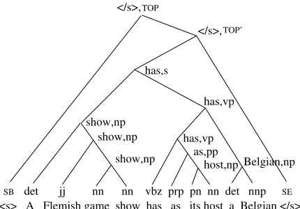
The CONSTRUCTOR builds the partial parseTk+1fromTk,wk+1, andtk+1 in a series of moves ending with NULL, where a parse moveais made with probabilityp(a|h−−1m);a∈A={(unary, NTlabel), (adjoin-left, NTlabel), (adjoin-right, NTlabel), NULL}. Depending on an actiona=adjoin-right or adjoin-left, the headwordh−1orh−2is percolated up by one tree level, the indices of the current exposed headwordsh−3,h−4,· · · are increased by 1, and these headwords together withh−1orh−2become the new exposed headwords. Once the CONSTRUCTOR hits NULL, the headword indexing and current parse structure remain as they are, and the CONSTRUCTOR passes control to the WORD-PREDICTOR.Figure 1
A complete parse tree by the structured language model.
A PLSA model (Hofmann 2001) is a generative probabilistic model of word-document co-occurrences using the bag-of-words assumption described as follows:
r
Choose a documentdwith probabilityp(d).r
SEMANTIZER selects a semantic classg∈Gwith probabilityp(g|d) whereGdenotes the set of topics.
r
WORD-PREDICTOR picks a wordw∈Vwith probabilityp(w|g).Because only one pair of (d,w) is being observed, the joint probability model is a mixture of log-linear models with the expression p(d,w)=p(d)gp(w|g)p(g|d). Typically, the number of documents and the vocabulary size are much larger than the size of latent semantic class variables. Latent semantic class variables therefore function as bottleneck variables to constrain word occurrences in documents.
When combining n-gram, m-SLM, and PLSA together to build a composite generative language model under the directed MRF paradigm (Wang et al. 2005b, 2006), the composite language model is simply a complicated generative model that has four operators: WORD-PREDICTOR, TAGGER, CONSTRUCTOR, and SEMANTIZER. The TAGGER and CONSTRUCTOR in SLM and the SEMANTIZER in PLSA remain unchanged; the WORD-PREDICTORs in n-gram, m-SLM, and PLSA, however, are combined to form a stronger WORD-PREDICTOR that generates the next word,wk+1, not only depending on themmost recently exposed headwordsh−−1m in the word-parse k-prefix but also itsn-gram historywkk−n+2and its semantic contentgk+1. The parameter for WORD-PREDICTOR in the composite n-gram/m-SLM/PLSA language model becomesp(w|w−−n1+1h−−1mg). The resulting composite language model has an even more complex dependency structure but with more expressive power than the original SLM. Figure 2 illustrates the structure of a compositen-gram/m-SLM/PLSA language model.
Figure 2
A compositen-gram/m-SLM/PLSA language model where the hidden information is the parse treeTand semantic contentg. Then-gram encodes local word interactions, them-SLM models the sentence’s syntactic structure, and the PLSA captures the document’s semantic content; all interact together to constrain the generation of natural language. The WORD-PREDICTOR generates the next wordwk+1with probabilityp(wk+1|wkk−n+2h
−1
−mgk+1) instead ofp(wk+1|wkk−n+2),
p(wk+1|h− 1
−m), andp(wk+1|gk+1), respectively.
normalization constraints for the parameters of each model component, WORD-PREDICTOR, TAGGER, CONSTRUCTOR, and SEMANTIZER. That is,
w∈V
p(w|w−−1n+1h−−1mg)=1 (2)
t∈O
p(t|wh−−1m.tag)=1 (3)
a∈A
p(a|h−−1m)=1 (4)
g∈G
p(g|d)=1 (5)
If we look at the example in Figure 1, for the composite n-gram/m-SLM/PLSA language model there exists a SEMANTIZER’s action to choose a topic g before any WORD-PREDICTOR’s action. Moreover, for m-SLM, its WORD-PREDICTOR predicts the next word, such as a, based on m most recently exposed headwords “s-SB, show-np, has-vp,” but for the composite model, the WORD-PREDICTOR predicts the next word a based on m most recently exposed headwords “s-SB, show-np, has-vp,”n-grams “as its host,” and a topicg. These are the only differences between SLM and our proposed composite language model.
3. Training Algorithm
For the composite n-gram/m-SLM/PLSA language model under the directed MRF paradigm, the likelihood of a training corpus D, a collection of documents, can be written as
ˆ
L(D,p)=
d∈D
l
Gl
Tl
Pp(Wl,Tl,Gl|d)
p(d)
where (Wl,Tl,Gl|d) denotes the joint sequence of thelth sentenceWlwith its parse struc-tureTland semantic annotation stringGlin documentd. This sequence is produced by a unique sequence of model actions: WORD-PREDICTOR, TAGGER, CONSTRUCTOR, SEMANTIZER moves; its probability is obtained by chaining the probabilities of these moves
Pp(Wl,Tl,Gl|d)=
g∈G
p(g|d)#(g,Wl,Gl,d) h−1,···,h−m∈H
(7)
w,w−1,···,w−n+1∈V
p(w|w−−1n+1h−−1mg)#(w−1−n+1wh −1 −mg,W
l,Tl,Gl,d)
t∈O
p(t|wh−−1m.tag)#(t,wh−1−m.tag,W
l,Tl,d)
a∈A
p(a|h−−1m)#(a,h−1−m,W l,Tl,d)
where #(g,Wl,Gl,d) is the count of semantic contentgin semantic annotation stringGlof thelth sentenceWlin documentd; #(w−−1n+1wh−−1mg,Wl,Tl,Gl,d) is the count ofn-grams, itsmmost recently exposed headwords, and semantic contentgin parseTland semantic annotation stringGlof thelth sentenceWlin documentd; #(twh−−1m.tag,Wl,Tl,d) is the count of tagtpredicted by wordwand the tags ofmmost recently exposed headwords in parse treeTlof thelth sentenceWlin documentd; and finally #(ah−−1m,Wl,Tl,d) is the count of constructor moveaconditioning onmexposed headwordsh−−1min parse treeTl of thelth sentenceWlin documentd.
Let
L(D,p)=
d∈D
l
Gl
Tl
Pp(Wl,Tl,Gl|d)
(8)
then
ˆ
L(D,p)=L(D,p) d∈D
p(d) (9)
Clearly, when maximizing ˆL(D,p) in Equation (6), p(d) is an ancillary term that is independent of all other data-generating parameters, it is not critical to anything that follows; moreover, when a language model is used to find the most likely word se-quence in machine translation and speech recognition, this term is useless. Thus, similar to ann-gram language model, we will generally ignore this term and concentrate on optimizing Equation (8) in the subsequent development.
The objective of maximum likelihood estimation is to maximize the likelihood
semantic content are hidden and the number of parse trees grows faster than expo-nentially with sentence length; Wang et al. (2006) have derived a generalized inside– outside algorithm by applying the standard EM algorithm and considering the auxiliary function
Q(p,p)=
d∈D l Gl Tl
Pp(Tl,Gl|Wl,d) logPp(Wl,Tl,Gl|d) (10)
The complexity of this algorithm is sixth order (sentence length), however; thus it is computationally too expensive to be practical for a large corpus even with the use of pruning on charts (Jelinek and Chelba 1999; Jelinek 2004).
3.1N-best List Approximate EM
Similar to SLM (Chelba and Jelinek 1998, 2000; Chelba 2000), we adopt anN-best list approximate EM re-estimation with modular modifications to seamlessly incorporate the effect of n-gram and PLSA components. Instead of maximizing the likelihood
L(D,p), we maximize theN-best list likelihood,
max
T
N
L(D,p,TN)=
d∈D
l max
Tl N∈TN
Gl
Tl∈Tl
N,||TlN||=N
Pp(Wl,Tl,Gl|d) (11)
whereTlN is a set ofN parse trees for sentenceWl in document d, || · ||denotes the cardinality, andTNis a collection ofT
l
N for sentences over entire corpusD. TheN-best list approximate EM involves two steps:
1. N-best list search: For each sentenceWin documentd, findN-best parse trees,
Tl
N =arg max
Tl N Gl
Tl∈Tl N
Pp(Wl,Tl,Gl|d),||T l N||=N
and denoteTNas the collection ofN-best list parse trees for sentences over entire corpusDunder model parameterp.
2. EM update: Perform one iteration (or several iterations) of the EM algorithm to estimate model parameters that maximizeN-best list likelihood of the training corpusD,
˜
L(D,p,TN)=
d∈D l Gl
Tl∈Tl N∈TN
That is,
(a) E-step: Compute the auxiliary function of theN-best list likelihood
˜
Q(p,p,TN)=
d∈D
l
Gl
Tl∈Tl N∈TN
Pp(Tl,Gl|Wl,d) logPp(Wl,Tl,Gl|d)
(b) M-step: Maximize ˜Q(p,p,TN) with respect topto get the new update forp.
Iterate steps (1) and (2) until the convergence of theN-best list likelihood.
We use Zangwill’s global convergence theorem (Zangwill 1969) to analyze the behavior of convergence of theN-best list approximate EM.
First, we define two concepts needed for Zangwill’s global convergence theorem. A mapM is from points of Θto subsets of Θ is called a point-to-set mapon Θ. It is said to be closed at θ if θi→θ,θi∈Θ and λi→λ,λi∈M(θi) implies λ∈M(θ). For a point-to-point map, continuity implies closedness. Then the global convergence theorem (Zangwill 1969) states the following.
Theorem
Let M be a point-to-set map (an algorithm) that, given a point θ0 ∈Θ, generates a sequence{θ∞i=0}through the iterationθi+1=M(θi). LetΩ∈Θbe the set of fixed points of M. Suppose (i) M is closed over the complement of Ω; (ii) there is a continuous function φonΘsuch that (a) ifθ /∈Ω,φ(λ)> φ(θ) for allλ∈M(θ), and (b) ifθ∈Ω, φ(λ)≥φ(θ) for allλ∈M(θ).
Then all the limit points of{θi}are inΩandφ(θi) converges monotonically toφ(θ) for someθ∈Ω.
Proof
This theorem has been used by Wu (1983) to prove the convergence of a standard EM algorithm (Dempster, Laird, and Rubin 1977). We now use this theorem to show that theN-best list approximate EM algorithm globally converges to the stationary points of theN-best list likelihood. We encounter one difficulty at this point, however, due to the maximization operator in Equation (11); after each iteration theN-best list may have been changed, therefore the set of data presented for the estimation of model parameters may be different from the previous one. Nevertheless, we prove the convergence of the N-best list approximate EM algorithm by checking whether it satisfies two conditions in Zangwill’s global convergence theorem. Because the composite model is essentially a mixture model of a curved exponential family through a complex hierarchy, there is a closed form solution for the ˜Q(p,p,TN) function irrespective of the N-best list parse trees, so theN-best list approximate EM algorithm is a one-to-one map. Because
˜
Q(p,p,TN) is continuous in both p and p, the map is closed, thus condition (i) is satisfied.
ofN-best list parse trees for sentences over entire corpusDunder two model parameters ˇ
pand ¯p, respectively:
ˇ
TN =arg max
T
N
L(D, ˇp,TN) (12)
¯
TN =arg max
T
N
L(D, ¯p,TN) (13)
and let ¯pbe the closed form solution of maximizing ˜Q(p, ˇp, ˇTN) with respect top, that is,
¯
p=arg max p
˜
Q(p, ˇp, ˇTN) (14)
Then
max
TN L(D, ¯p,T
N)≥L˜(D, ¯p, ˇTN) (15)
≥L˜(D, ˇp, ˇTN) (16)
≥max
T
N
L(D, ˇp,TN) (17)
The inequality in Equation (15) is strict unless ˇTN=T¯N, which results in ¯p∈M( ¯p). Using results proven by Wu (1983), we know that when ˇpis not a stationary point of the N-best list likelihood or ˇp∈/M( ˇp), ∂L˜(D, ˇp,TN)
∂pˇ =
∂Q˜(p, ˇp, ˇTN)
∂pˇ =0, ˜Q( ¯p, ˇp, ˇTN)>Q˜( ˇp, ˇp, ˇTN), thus the inequality in Equation (16) is strict. Finally, the inequality in Equation (17) is strict unless ˇp∈M( ˇp). Thus condition (ii) is satisfied.
This completes the proof that the N-best list approximate EM algorithm mono-tonically increases theN-best list likelihood and converges in the sense of Zangwill’s global convergence.
In the following, we formally derive theN-best list approximate EM algorithm with linear sentence length time complexity.
3.1.1N-best List Search Strategy.For each sentenceWin documentd, instead of scanning all the hidden events (both allowed parse trees and semantic annotation strings) we restrict the algorithm to operate with N-best hidden events. We find that, for each document, a large number of topics should be pruned and only a small set of allowed topics should be kept due to the considerations of both computational time and resource demand, otherwise we have to use many more machines to store WORD-PREDICTOR’s parameters.
We can either find both theN-best parses for each sentence and N-best topics for each document simultaneously or separately. The latter is much preferred, because the first case is much more computationally expensive.
To extract theN-best topics, we run an EM algorithm for a PLSA model on training corpusD, then keep theNmost likely topics (denoted asGd) according to the values of p(g|d); the rest of the topics are purged.
hypotheses (partial parses) that have been constructed by the same number of WORD-PREDICTOR and the same number of CONSTRUCTOR operations. The hypotheses in each stack are ranked according to the log(Pp(Wk,Tk|d)) score with the highest on top, wherePp(Wk,Tk|d)=
GkPp(Wk,Tk,Gk|d) and theWk,Tk,Gkdenote the joint sequence of prefixWk=w0,w1· · ·,wkwith its parse structureTkand semantic annotation string Gk=g1,· · ·,gk, gi∈Gd,i=1,· · ·,k in document d. This sequence is produced by a unique sequence of model actions: WORD-PREDICTOR, TAGGER, CONSTRUCTOR, and SEMANTIZER moves. Its probability is obtained by chaining the probabilities of these moves. The value ofPp(Wk,Tk|d) is computed recursively fromPp(Wk−1,Tk−1|d) by the following formula:
Pp(Wk,Tk|d)=Pp(Wk−1,Tk−1|d)
gk∈Gd
p(wk|wkk−−1n+1h−−1mgk) p(gk|d) gi∈Gdp(gi|d)
(18)
p(tk|wk,h−−1m.tag)p(Tk−1,k|Wk−1Tk−1,wk,tk)
where Wk−1Tk−1 is the word-parse (k−1)-prefix; wk is the kth word predicted by WORD-PREDICTOR;tkis the tag assigned to wkby the TAGGER;Tk−1,k is the incre-mental parse structure that generates Tk=Tk−1||Tk−1,k when attached to Tk−1, (this is the parse structure built on top of Tk−1 and the newly predicted word wk); the || notation stands for concatenation. Finally, p(Tk−1,k|Wk−1Tk−1,wk,tk) is the product of the probabilities of a series of CONSTRUCTOR moves inTk−1,kto formTk. Because the topics are pruned toGd, the probability of the SEMANTIZER is normalized to ensure a proper probability distribution. A stack vector consists of the ordered set of stacks con-taining partial parses with the same number of WORD-PREDICTOR operations but a different number of CONSTRUCTOR operations. In WORD-PREDICTOR and TAGGER operations, some hypotheses are discarded due to the maximum number of hypotheses that the stack can contain at any given time. In the CONSTRUCTOR operation, the resulting hypotheses are discarded due to either finite stack size or the log-probability threshold (the maximum tolerable difference between the log-probability score of the top-most hypothesis and the bottom-most hypothesis at any given state of the stack). The synchronous, multi-stack search strategy is a greedy best-first search algorithm, one of the local heuristic search procedures that does not use future cost estimates to guide the search and thus does not guarantee that theN-best list parse trees are a global optimal solution (Russell and Norvig 2010). In practice, however, we find that theN-best list approximate EM algorithm does converge within several iterations.
3.1.2 EM Update.Once we have both theN-best parse trees for each sentence in docu-mentdand theN-best topics for documentd, we derive the EM algorithm to estimate model parameters.
Maximizing ˜Q(p,p,TN) with respect topleads to re-estimated parameters of the composite model, which are nothing but the following normalized conditional expected counts:
p(w|w−−1n+1h−−1mg)∝ d∈D
l
Gl
Tl∈Tl N∈TN
Pp(Tl,Gl|Wl,d)#(w−−1n+1wh
−1
−mg,W l
p(t|wh−−1m.tag)∝ d∈D
l
Tl∈Tl N∈TN
Pp(Tl|Wl,d)#(twh−−1m.tag,W l
,Tl,d) (20)
p(a|h−−1m))∝
d∈D
l
Tl∈Tl N∈TN
Pp(Tl|Wl,d)#(ah−−1m,W l
,Tl,d) (21)
p(g|d)∝ d∈D
l
Gl
Tl∈Tl N∈TN
Pp(Tl,Gl|Wl,d)#(g,Wl,Gl,d) (22)
In the E-step, we use Equations (19)–(22) to compute the expected count of each model parameter over sentenceWlin documentdin the training corpusD. In the full case where the number of parse trees grows faster than exponentially with sentence length, we use Jelinek-style recursive formulas in the generalized inside–outside algo-rithm (Jelinek 2004) to handle the tree structure and describe the weighted forest of possible derivations (Wang et al. 2006). In theN-best list case considered in this paper, however, we just enumerate each parse tree in theN-best list and compute the expected posterior count for each parse tree. For the WORD-PREDICTOR and the SEMANTIZER, we use Equations (19) and (22) and note that there is a sum over semantic annotation se-quenceGlwhere the number of possible semantic annotation sequences is exponential. We use forward–backward recursive formulas reminiscent of those in hidden Markov models to compute the expected counts. To be more specific, for each parseTl∈TNl, we define the forward vectorαl(g|d) to be
αlk+1(g|d)= Gl
k
Pp(Wkl,T l k,w
k
k−n+2wk+1h−−1mg,G l
k|d) (23)
=Pp(Wlk,T l k,w
k
k−n+2wk+1h−−1mg|d)
=Pp(Wlk,T l
k|d)p(wk+1|wkk−n+2h
−1
−mg,d)
p(gk+1|d)
gi∈Gdp(gi|d)
whereWlkis the wordk-prefix for sentenceWl, andTlkis the parse fork-prefix. It is easy to see that the forward vectorαl(g|d) can be recursively computed in a forward manner using Equation (18) as
αlk+1(g|d)=
gk∈Gd
αlk(gk|d)
p(tk|wk,h−−1m.tag)p(T l k−1,k|W
l k−1T
l
k−1,wk,tk) (24)
p(wk+1|wkk−n+2h
−1
−mg,d)
p(gk+1,d)
gi∈Gdp(gi|d)
We define the backward vectorβl(g|d) to be
βlk+1(g|d)= Gl
k+1,·
Pp(Wkl+1,·,T l k+1,·,G
l k+1,·|w
k
k−n+2wk+1h−−1mg,d) (25)
Wlk+1that generates parse treeTl,Tl=Tkl+1||Tlk+1,·, andGlk+1,·=gk+2,· · ·, is the seman-tic subsequence inGlrelevant toWlk+1,·. Again it is easy to see that the backward vector βl(g|d) can be recursively computed in a backward manner as
βlk+1(g|d)=p(tk+1|wk+1,h−−1m.tag)p(T l k,k+1|W
l kT
l
k,wk+1,tk+1) (26)
gk+2∈Gd
p(wk+2|wkk−n+3h
−1
−mgk+2,d)
p(gk+2|d)
gi∈Gdp(gi|d)
Gl k+2,·
Pp(Wlk+2,·,T l k+2,·,G
l k+2,·|w
k+1
k−n+3wk+2h
−1
−mgk+2,d)
=p(tk+1|wk+1,h−−1m.tag)p(T l k,k+1|W
l kT
l
k,wk+1,tk+1)
gk+2∈Gd
p(wk+2|wkk−n+3h
−1
−mgk+2,d)
p(gk+2|d)
gi∈Gdp(gi|d)
βlk+2(gk+2|d)
Then, the expected count ofw−−1n+1wh−−1mgfor the WORD-PREDICTOR on sentenceWl in documentdis
Gl
Tl∈Tl N∈TN
Pp(Tl,Gl|Wl,d)#(w−−1n+1wh
−1
−mg,W l
,Tl,Gl,d) (27)
=
Gl
Tl∈Tl N∈TN
Pp(Tl,Gl,Wl|d)#(w−−1n+1wh
−1
−mg,W l
,Tl,Gl,d)/Pp(Wl|d)
=
l
k
αlk+1(g|d)βlk+1(g|d)δ(wkk−n+2wk+1h− 1
−mgk+1=w− 1
−n+1wh
−1
−mg)/Pp(Wl|d)
wherePp(Wl|d)=Gl
Tl∈Tl
N∈TNPp(T
l,Gl,Wl|d)= Tl∈Tl
N∈TNPp(T
l,Wl|d),P
p(Tl,Wl|d) is recursively computed by Equation (18) through traversing thelth parse treeTl∈TNl of sentenceWlfrom left to right, andδ(·) is an indicator function. The expected count ofgfor the SEMANTIZER on sentenceWlin documentdis
Gl
Tl∈Tl N∈TN
Pp(Tl,Gl|Wl,d)#(g,Wl,Gl,d) (28)
=
l
k
αlk+1(g|d)βlk+1(g|d)p(wk+1|wkk−n+2h
−1
−mg)/Pp(Wl|d)
For the TAGGER and the CONSTRUCTOR, we use Equations (20) and (21), and the expected count of each event of twh−−1m.tag and ah−−1m over parse Tl of sentence Wl in documentdis the real count appearing in parse treeTl of sentenceWlin documentd times the conditional distributionPp(Tl|Wl,d)=Pp(Tl,Wl|d)/Tl∈TlPp(Tl,Wl|d)—that is,Pp(Tl|Wl,d)#(twh−−1m.tag,Wl,Tl,d) andPp(Tl|Wl,d)#(ah−−1m,Wl,Tl,d), respectively.
times the posterior probabilityPp(Tl|Wl,d), as is done in Chelba and Jelinek (1998, 2000) and Chelba (2000).
In the M-step, the recursive linear interpolation scheme (Jelinek and Mercer 1980) is used to obtain a smooth probability estimate for each model component (WORD-PREDICTOR, TAGGER, and CONSTRUCTOR). The TAGGER and CONSTRUCTOR are conditional probabilistic models of the typep(u|z1,· · ·,zn) whereu,z1,· · ·,znbelong to a mixed set of words, POS tags, NTtags, and CONSTRUCTOR actions (u only); and z1,· · ·,znform a linear Markov chain. The recursive mixing scheme is the standard one among relative frequency estimates of different ordersk=0,· · ·,n and has been ex-plained in Chelba and Jelinek (1998, 2000) and Chelba (2000). The WORD-PREDICTOR is, however, a conditional probabilistic modelp(w|w−−n1+1h−−1mg) where there are three kinds of context, w−−1n+1,h−−1m, and g—each forms a linear Markov chain. The model has a combinatorial number of relative frequency estimates of different orders among three linear Markov chains. We generalize Jelinek and Mercer’s (1980) original recur-sive mixing scheme to handle the situation where the context is a mixture of Markov chains. The factored language (FL) model (Bilmes and Kirchhoff 2003) is close to the smoothing technique we propose here, the major difference is that FL considers all possible combination of the context of conditional probability that can be concisely represented by a factor graph, whereas our approach strictly respects the order of Markov chains for word sequence and headword sequence because we believe natural language tightly follows these orders; moreover, where FL uses a backoff technique, we use linear interpolation.
[image:15.486.54.289.373.588.2]Consider a composite trigram/2-SLM/PLSA language model. Figure 3 illustrates a lattice formed of all possible conditional probabilistic models and relative frequency
Figure 3
Recursive linear interpolation lattice to estimate WORD-PREDICTORp(w|w−2w−1h−2h−1g) of
the composite trigram/2-SLM/PLSA language model, whereUis the vocabulary in which the predicted random variablewtakes values andp(U) denotes uniform distribution ofU. The lattice is formed by three linear Markov chains,w−2w−1,h−2h−1, andg. Starting fromp(U),
estimates of different orders along each of the three linear Markov chains. Each vertex in the lattice represents a conditional probabilistic model that is a linear interpolation of vertices having directed arcs pointing to this vertex and its relative frequency estimate; the linear interpolation coefficients are the weights of directed arcs. For example, the WORD-PREDICTORp(w|w−2w−1h−2h−1g) is a linear interpolation of three conditional probabilistic models, p(w|w−1h−2h−1g), p(w|w−2w−1h−1g), p(w|w−2w−1h−2h−1), and their relative frequency estimatef(w|w−2w−1h−2h−1g),
p(w|w−2w−1h−2h−1g)=λw(w−2w−1h−2h−1g)·p(w|w−1h−2h−1g) (29) +λh(w−2w−1h−2h−1g)·p(w|w−2w−1h−1g)
+λg(w−2w−1h−2h−1g)·p(w|w−2w−1h−2h−1) +(1−λw(w−2w−1h−2h−1g)−λh(w−2w−1h−2h−1g)
−λg(w−2w−1h−2h−1g))·f(w|w−2w−1h−2h−1g)
where λw(w−2w−1h−2h−1g),λh(w−2w−1h−2h−1g), and λg(w−2w−1h−2h−1g) are non-negative context-dependent interpolation coefficients with a sum of less than 1;
f(w|w−2w−1h−2h−1g)=
C(w−2w−1wh−2h−1g)
C(w−2w−1h−2h−1g); and C(w−2w−1wh−2h−1g) is the expected count of the event w−2w−1wh−2h−1g that is extracted from the training cor-pus by the E-step of the N-best approximate EM algorithm, C(w−2w−1h−2h−1g)=
w∈UC(w−2w−2wh−2h−1g). The linear interpolation coefficients are grouped into equivalence classes (tied) based on the range into which the count falls; the count ranges for each equivalence class, “buckets,” are set such that a statistically sufficient number of events fall within that range. In our experiments, we set the count ranges to be the intervals of 2i,i=0, 1,· · ·, 10 (i.e., 0, 1, 2, 4, 8, 16, 32, 64, 128, 256, 512, 1024, and∞). These “tied” interpolation weights are determined by the maximum likelihood estimate from cross-validation data through the EM algorithm (Dempster, Laird, and Rubin 1977) where we use a public available parser in the openNLP software1to parse sentences in cross-validation data, and we run LSA to extractNmost likely topics for each document in cross-validation data, then we gather joint counts for each model component, WORD-PREDICTOR, TAGGER, CONSTRUCTOR used to determine interpolation weights.
In the M-step, assuming that the count ranges and the corresponding interpolation values for each order are kept fixed to their initial values, the only parameters to be re-estimated using the EM algorithm are the maximal order counts for each model component. The interpolation scheme outlined here is then used to obtain a smooth probability estimate for each model component.
3.2 Follow-up EM
As explained in Chelba and Jelinek (2000) and Chelba (2000), for the SLM component a large fraction of the partial parse trees that can be used for assigning probability to the next word do not survive in the synchronous, multi-stack search strategy, thus they are not used in the N-best approximate EM algorithm for the estimation of WORD-PREDICTOR to improve its predictive power. To remedy this weakness, we estimate a
separate WORD-PREDICTOR (and SEMANTIZER) model using the partial parse trees exploited by the synchronous, multi-stack search strategy.
First, we look at how to compute thelanguage modelprobability assignment for the word at positionk+1 in the input sentence of documentdwhen the word-parsek-prefix WkTkis available. From the causal relationship among the parameters of the composite n-gram/m-SLM/PLSA, we have
Pp(wk+1|Wk,d)=
Tk∈Zk,gk+1∈Gd
Pp(wk+1,Tk,gk+1|Wk,d) (30)
=
Tk∈Zk,gk+1∈Gd
Pp(wk+1|Wk,Tk,gk+1,d)Pp(Tk|Wk,d)
p(gk+1|d)
gi∈Gdp(gi|d)
=
h−1−m∈Tk;Tk∈Zk,gk+1∈Gd
p(wk+1|wkk−n+2h
−1
−mgk+1)Pp(Tk|Wk,d)
p(gk+1|d)
gi∈Gdp(gi|d)
wherePp(Tk|Wk,d)=
GkPp(Wk,Tk,Gk|d)
Tk∈Zk
GkPp(Wk,Tk,Gk|d) to ensure a proper probability normaliza-tion over word stringsWk;Zkis the set of all parses present in the stacks at the current stage k during the synchronous multi-stack pruning strategy and it is a function of the wordk-prefixWk=w0,· · ·,wk;Gk=g1,· · ·,gk,gi∈Gd,i=1,· · ·,kis the semantic string up tok; andPp(Wk,Tk,Gk|d) is the joint probability of word-parsek-prefixWkTk and its semantic stringGkin a documentd.
The likelihood of a training corpusDunder this language model probability as-signment that uses partial parse trees generated during the process of the synchronous, multi-stack search strategy can be written as
˜
L(D,p)=
d∈D
l
Pp(Wl|d)
(31)
wherePp(Wl|d)=
kPp(w (l) k+1|W
l
k,d) andW
l is thelth sentence in documentd. Again, similar to Equation (8), we ignore the ancillary termp(d) in Equation (31).
We use a second stage of parameter re-estimation for p(wk+1|wkk−n+2h
−1
−mgk+1) and p(gk+1|d) by maximizing Equation (31) to improve WORD-PREDICTOR’s predictive power. In this case, the estimation of the WORD-PREDICTOR is for the emission probability of a hidden Markov model with fixed transition probabil-ities (although dependent on the position k in the input sentence) specified by the Pp(Tk|Wk,d)
p(gk+1|d)
gi∈Gdp(gi|d) values. We use EM again. The E-step is to gather expected joint counts C(wkk−n+2wk+1h−
1
−mgk+1,d) and C(gk+1,d) of the WORD-PREDICTOR model by accumulating each count at positionk weighted by a posterior probability Pp(Tk,gk+1|wk+1,Wk,d), namely,
Pp(Tk,gk+1|wk+1,Wk,d)=
p(wk+1|wkk−n+2h
−1
−mgk+1)p(gk+1|d)Pp(Tk|Wk,d)
h−1−m∈Tk∈Zk,g∈Gdp(wk+1|w k k−n+2h
−1
−mg)p(g|d)Pp(Tk|Wk,d)
3.3 Distributed Architecture
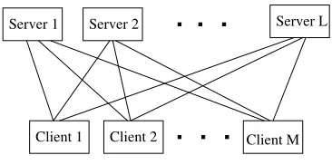
When using very large corpora to train our composite language model, the data and the parameters cannot be stored together on a single machine, so we have to resort to dis-tributed computing. The topic of large-scale disdis-tributed language models is relatively new, and existing work is restricted to n-grams only (Zhang, Hildebrand, and Vogel 2006; Brants et al. 2007; Emami, Papineni, and Sorensen 2007). Although all existing research use distributed architectures that follow the client–server paradigm, the real implementations are in fact different. Zhang et al. (2006) and Emami et al. (2007) store training corpora in suffix arrays such that one sub-corpus per server serves raw counts, and test sentences are loaded in a client. This implies that when computing the language model probability of a sentence in a client, all servers need to be contacted for each n-gram request. The approach by Brants et al. (2007) follows a standard MapReduce paradigm (Dean and Ghemawat 2004): The corpus is first divided and loaded into a number of clients, andn-gram counts are collected at each client, then then-gram counts are mapped via hashing and are stored in a number of servers, resulting in exactly one server being contacted per n-gram when computing the language model probability of a sentence. We adopt a similar approach to Brants et al. (2007) and make it suitable to perform iterations of the N-best list approximate EM algorithm (see Figure 4). The corpus is divided and loaded into a number of clients. We use a publicly available parser to parse the sentences in each client to get the initial counts for w−−1n+1wh−−1mg (WORD-PREDICTOR),twh−−1m.tag (TAGGER), andah−−1m (CONSTRUCTOR), we finish the Map part, and then the counts for a particularw−−1n+1wh−−1mgat different clients are summed up and stored in one of the servers by hashing through wordw−1, headword
h−1, and its topic g. The counts for all twh−−1m.tag and ah− 1
[image:18.486.49.232.508.599.2]−m at different clients are summed up and stored in one of the servers, then we complete the Reduce part. This is the initialization of the N-best list approximate EM step. Each client then calls the servers for parameters to perform a synchronous multi-stack search for each sentence to get theN-best list parse trees. Again, the expected count for a particular parameter of w−−1n+1wh−−1mg,twh−−1m.tag, andah−−1mat the clients are computed, thus we finish the Map part. The expected count ofw−−1n+1wh−−1mgare then summed up and stored in one of the servers by hashing through wordw−1, headwordh−1, and its topicg, and the counts for all twh−−1m.tag and ah−−1m at different clients are summed up and stored in one of the servers; thus we finish the Reduce part. The SEMANTIZER has document-specific
Figure 4
Distributed architecture is essentially a MapReduce paradigm: Clients store partitioned data and perform the E-step: compute expected counts; this is “Map.” Servers store parameters (counts) for the M-step where counts ofw−−1n+1wh
−1
−mgare hashed by wordw−1, headwordh−1, and its
parameters, thus the EM iterative updates are performed at each of local clients. We repeat this procedure until convergence.
Similarly, we use a distributed architecture as in Figure 4 to perform the follow-up EM algorithm to re-estimate WORD-PREDICTOR.
4. Using the Model for Testing
When a language model is used in one-pass decoders of speech recognition and phrased-based MT systems to guide the search, the search space is organized as a prefix tree and operates left to right, thus we need to know the language model probability at the word level given by Equation (30) one word at a time. Because a document of the test data is not contained in the original training corpus, to compute the language model probability assignment for word wk+1 we use a “fold-in” heuristic approach similar to the one used in Hofmann (2001): The parameters corresponding to SEMANTIZER, p(g|d), are re-estimated by maximizing the probability of word subsequence seen so far—that is, a pseudo-document ˜dk=(Wk,S), whereSis the set of previous sentences of a document in test data—while holding the other parameters fixed. Wang et al. (2005b) use on-line gradient ascent to re-estimate these parameters. We use three methods, one-step on-line EM, on-line EM with fixed learning rate, and batch EM, to re-estimate these parameters. Both one-step on-line EM and on-line EM with fixed learning rate use Equation (32) withγset to 1
|d˜
k|+1
and a constant 0.2, respectively.
p(g|d˜k)=γ
h−1−m∈Tk−1;Tk−1∈Zk−1p(wk|w k−1 k−n+1h
−1
−mg)p(g|d˜k−1)Pp(Tk−1|Wk−1, ˜dk−1)
g∈Gd
h−1−m∈Tk−1;Tk−1∈Zk−1p(wk|w k−1 k−n+1h
−1
−mg)p(g|d˜k−1)Pp(Tk−1|Wk−1, ˜dk−1)
+(1−γ)p(g|d˜k−1) (32)
The batch EM is the standard EM algorithm where we repeat the iterative procedure
until convergence. The initial values are set to
d∈D#(d) p(g|d)
gi∈Gdp(gi|d)
|D| , where for the topics
that are purged we just plug in 0 forp(g|d). #(d) is the number of words in document d,d∈D, and |D|=d#(d) denotes the size of training corpus (which is the total number of words in the entire training corpus).
When we use Equation (30) to compute perplexity, the system only uses information coming from previous words to generate a topic distribution, which then is used to predict the next word, so the sum over all next words is 1.
We find that the perplexity results are sensitive to these three methods and the initial values. For example, for batch EM, if we set initial values to be those obtained by using the pseudo-document up to the previous word ˜dk−1=(Wk−1,S) and trained by batch EM, we obtain worse perplexity results. Table 8 in Section 6.2 gives perplexity results that use these three methods to re-estimate the parameters of the SEMANTIZER, where the on-line EM with fixed learning rate not only has the cheapest computational cost but also leads to the highest perplexity reductions.
5. Related Work
SLM and a word clustering model to extract relevant grammatical and semantic fea-tures, then integrated these features withn-grams by a maximum conditional entropy approach. Our composite language model is a generative model, all features play impor-tant roles in the EM iterations to allow maximal order events for WORD-PREDICTOR to appear; in Khudanpur and Wu (2000), however, the counts for all events are fixed after feature extraction from SLM and word clustering and no new maximal order events for WORD-PREDICTOR are possibly extracted, this potentially hinders the predictive power of WORD-PREDICTOR. Moreover, the training algorithm in Khudanpur and Wu is computationally expensive. Both methods use the first-stageN-best list approximate EM to extract headwords, thus the complexity is at the same order at this stage; at second stage, however, where we use the follow-up EM, they use the maximum en-tropy approach. The maximum enen-tropy approach is more expensive, mainly in feature expectation and normalization as well as optimization (such as iterative scaling or the quasi Newton method); ours is quite simple, which is expected relative to frequency estimates with proper smoothing.
The highest reported perplexity reductions are those by Goodman (2001), where the author examines the techniques of caching, clustering, higher-ordern-grams, skipping models, and sentence-mixture models in various combinations (mainly linear interpola-tion). The authorcompares to the baseline of a Katz smoothed trigramwith no count cutoffs. On a small training corpus with 100k tokens, a 50% perplexity reduction (1 bit improve-ment) is obtained. On a larger corpus with 284 million tokens without punctuation, the improvement declines to 38%; we assume that this improvement shrinks to 30% when compared with 4-gram as the baseline.
6. Experimental Results
In this section, we first explain the experimental set-up for our experiments, we then show comprehensive perplexity results in various situations, and we end by reporting the results when we apply the composite language model to the task of re-ranking the N-best list from a state-of-the-art parsing-based machine translation system.
6.1 Experimental Set-up
Table 1
The corpora used in our experiments.
1.3BILLION TOKEN TRAINING CORPUS
AFP 19940512.0003∼19961015.0568
AFW 19941111.0001∼19960414.0652
NYT 19940701.0001∼19950131.0483
NYT 19950401.0001∼20040909.0063
XIN 19970901.0001∼20041125.0119
230MILLION TOKEN TRAINING CORPUS
AFP 19940622.0336∼19961031.0797
APW 19941111.0001∼19960419.0765
NYT 19940701.0001∼19941130.0405
44MILLION TOKEN TRAINING CORPUS
AFP 19940601.0001∼19950721.0137
13.7MILLION TOKEN CHECK CORPUS
NYT 19950201.0001∼19950331.0494
1.7MILLION TOKEN CHECK CORPUS
AFP 19940512.0003∼19940531.0197
354K TOKEN TEST CORPUS
CNA 20041101.0006∼20041217.0009
These are selected from the LDC English Gigaword corpus. AFP = Agence France-Presse; AFW = Associated Press Worldstream; NYT = New York Times; XIN = Xinhua News Agency; and CNA = Central News Agency of Taiwan denote the sections of the LDC English Gigaword corpus.
The vocabulary sizes in all three cases are:
r
word (also WORD-PREDICTOR operation) vocabulary: 60k, open— all words outside the vocabulary are mapped to theunktoken, these 60k words are chosen from the most frequently occurring words in the 44 million token corpus;r
POS tag (also TAGGER operation) vocabulary: 69, closed;r
non-terminal tag vocabulary: 54, closed;r
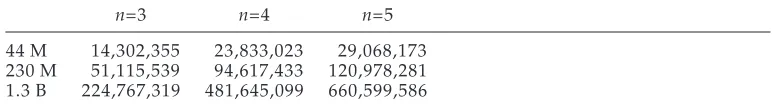
CONSTRUCTOR operation vocabulary: 157, closed.Table 2
Statistics about the number of types ofn-grams (n=3, 4, 5) on the 44 million, 230 million, and 1.3 billion token corpora.
n=3 n=4 n=5
44 M 14,302,355 23,833,023 29,068,173 230 M 51,115,539 94,617,433 120,978,281 1.3 B 224,767,319 481,645,099 660,599,586
the 354k token test corpus is 2.0%. Table 2 lists the statistics about the number of types ofn-grams on these three corpora.
Similar to SLM (Chelba 2000; Chelba and Jelinek 2000), after the parse under-goes headword percolation and binarization, each model component of WORD-PREDICTOR, TAGGER, and CONSTRUCTOR is initialized from a set of parsed sentences. We use the openNLP software2 to parse a large number of sentences in the LDC English Gigaword corpus to generate an automatic treebank, which has a slightly different word-tokenization than that of the manual treebank such as the Penn Treebank used in Chelba and Jelinek (2000) and Chelba (2000). For the 44 and 230 million token corpora, all sentences are automatically parsed and used to initialize model parameters, whereas for the 1.3 billion token corpus, we parse the sentences from a portion of the corpus that contains 230 million tokens, then use them to initialize model parameters. The parser at openNLP is trained on the Penn Treebank, which has only one million tokens, and there is a mismatch between the Penn Treebank and the LDC English Gigaword corpus. Nevertheless, experimental results show that this approach is effec-tive to provide initial values of model parameters.
6.2 Perplexity Results
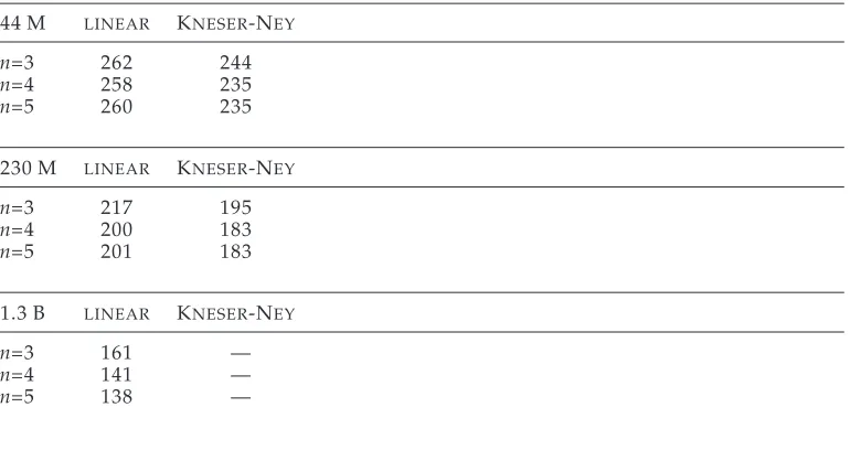
Table 3 gives the perplexity results (Bahl et al. 1977) ofn-grams (n= 3, 4, and 5) using linear interpolation and Kneser-Ney (1995) smoothing when the training corpus has 44 million, 230 million, and 1.3 billion tokens, respectively. We have implemented a distributedn-gram with linear interpolation smoothing, but we don’t have distributed n-grams with Kneser-Ney smoothing implemented by us. Instead, we use the SRI Language Modeling Toolkit to obtain perplexity results of n-grams with Kneser-Ney smoothing for the 44 million and 230 million token corpora using a single machine that has 20G memory at the Ohio Supercomputer center. We are not able to compute per-plexity results ofn-grams with Kneser-Ney smoothing on the 1.3 billion token corpus, thus we leave these results blank in Table 3. From the results in Table 3, we decided to use a linearly smoothed trigram as the baseline model for the 44 million token corpus, a linearly smoothed 4-gram as the baseline model for the 230 million token corpus, and a linearly smoothed 5-gram as the baseline model for the 1.3 billion token corpus.
As we mentioned in Section 3.1.1, we can keep only a small set of topics due to the considerations of computational time and resource demand. Table 4 shows the perplexity results and computation time of compositen-gram/PLSA language models that are trained on the three corpora when the pre-defined number of total topics is 200, but different numbers of most-likely topics are kept for each document in PLSA; the
Table 3
Perplexity results ofn-grams (n= 3, 4, and 5) using linear interpolation and Kneser-Ney
smoothing when training set is a 44 million, 230 million, or 1.3 billion token corpus, respectively.
44 M LINEAR KNESER-NEY
n=3 262 244
n=4 258 235
n=5 260 235
230 M LINEAR KNESER-NEY
n=3 217 195
n=4 200 183
n=5 201 183
1.3 B LINEAR KNESER-NEY
n=3 161 —
n=4 141 —
[image:23.486.53.437.373.500.2]n=5 138 —
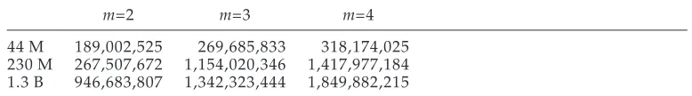
Table 4
Perplexity (ppl) results and time consumed of the compositen-gram/PLSA language model trained on three corpora when different numbers of most-likely topics are kept for each document in PLSA.
CORPUS n #OF PPL TIME #OF #OF #OF TYPES TOPICS (HOURS) SERVERS CLIENTS OFww−−1n+1g
44M 3 5 196 0.5 40 100 120.1M
3 10 194 1.0 40 100 218.6M 3 20 190 2.7 80 100 537.8M
3 50 189 6.3 80 100 1.123B
3 100 189 11.2 80 100 1.616B 3 200 188 19.3 80 100 2.280B 230M 4 5 146 25.6 280 100 0.681B 1.3B 5 2 111 26.5 400 100 1.790B 5 5 102 75.0 400 100 4.391B
rest are pruned. For the composite 5-gram/PLSA model trained on the 1.3 billion token corpus, 400 cores have to be used to keep the top five most likely topics. For the composite trigram/PLSA model trained on the 44M token corpus, the computation time increases drastically, with less than 5% percent perplexity improvement. In the following experiments, therefore, we keep the top five topics for each document from a total of 200 topics—all other 195 topics are pruned.