Learning Representations for Weakly Supervised Natural Language Processing Tasks

Supervised Natural Language

Processing Tasks

Fei Huang

Arun Ahuja

Northwestern University

Doug Downey

Yi Yang

Northwestern University

Yuhong Guo

Alexander Yates

Finding the right representations for words is critical for building accurate NLP systems when domain-specific labeled data for the task is scarce. This article investigates novel techniques for extracting features from n-gram models, Hidden Markov Models, and other statistical language models, including a novel Partial Lattice Markov Random Field model. Experiments on part-of-speech tagging and information extraction, among other tasks, indicate that features taken from statistical language models, in combination with more traditional features, outperform traditional representations alone, and that graphical model representations outperform n-gram models, especially on sparse and polysemous words.

∗1805 N. Broad St., Wachman Hall 324, Philadelphia, PA 19122, USA. E-mail:{fei.huang,yuhong,yates}@temple.edu.

∗∗2133 Sheridan Road, Evanston, IL, 60208. E-mail:[email protected]. †2133 Sheridan Road, Evanston, IL, 60208. E-mail:[email protected]. ‡2133 Sheridan Road, Evanston, IL, 60208. E-mail:[email protected].

Submission received: 13 June 2012; revised submission received: 25 November 2012, accepted for publication: 15 January 2013.

1. Introduction

NLP systems often rely on hand-crafted, carefully engineered sets of features to achieve strong performance. Thus, a part-of-speech (POS) tagger would traditionally use a feature like, “the previous token is the” to help classify a given token as a noun or adjective. For supervised NLP tasks with sufficient domain-specific training data, these traditional features yield state-of-the-art results. However, NLP systems are in-creasingly being applied to the Web, scientific domains, personal communications like e-mails and tweets, among many other kinds of linguistic communication. These texts have very different characteristics from traditional training corpora in NLP. Evidence from POS tagging (Blitzer, McDonald, and Pereira 2006; Huang and Yates 2009), parsing (Gildea 2001; Sekine 1997; McClosky 2010), and semantic role labeling (SRL) (Pradhan, Ward, and Martin 2007), among other NLP tasks (Daum´e III and Marcu 2006; Chelba and Acero 2004; Downey, Broadhead, and Etzioni 2007; Chan and Ng 2006; Blitzer, Dredze, and Pereira 2007), shows that the accuracy of supervised NLP systems degrades significantly when tested on domains different from those used for training. Collecting labeled training data for each new target domain is typically prohibitively expensive. In this article, we investigate representations that can be applied toweakly supervised learning, that is, learning when domain-specific labeled training data are scarce.

A growing body of theoretical and empirical evidence suggests that traditional, manually crafted features for a variety of NLP tasks limit systems’ performance in this weakly supervised learning for two reasons. First, feature sparsity prevents systems from generalizing accurately, because many words and features are not observed in training. Also because word frequencies are Zipf-distributed, this often means that there is little relevant training data for a substantial fraction of parameters (Bikel 2004b), espe-cially in new domains (Huang and Yates 2009). For example, word-type features form the backbone of most POS-tagging systems, but types like “gene” and “pathway” show up frequently in biomedical literature, and rarely in newswire text. Thus, a classifier trained on newswire data and tested on biomedical data will have seen few training examples related to sentences with features “gene” and “pathway” (Blitzer, McDonald, and Pereira 2006; Ben-David et al. 2010).

Further, because words are polysemous, word-type features prevent systems from generalizing to situations in which words have different meanings. For instance, the word type “signaling” appears primarily as a present participle (VBG) in Wall Street Journal (WSJ) text, as in, “Interest rates rose, signaling that . . . ” (Marcus, Marcinkiewicz, and Santorini 1993). In biomedical text, however, “signaling” appears primarily in the phrase “signaling pathway,” where it is considered a noun (NN) (PennBioIE 2005); this phraseneverappears in the WSJ portion of the Penn Treebank (Huang and Yates 2010).

the number of features that they produce, controlling how sparse those features are in training data.

Our specific contributions are as follows:

1. We show how to generate representations from a variety of language models, includingn-gram models, Brown clusters, and Hidden Markov Models (HMMs). We also introduce a Partial-Lattice Markov Random Field (PL-MRF), which is a tractable variation of a Factorial Hidden Markov Model (Ghahramani and Jordan 1997) for language modeling, and we show how to produce representations from it.

2. We quantify the performance of these representations in experiments on POS tagging in a domain adaptation setting, and weakly supervised information extraction (IE). We show that the graphical models outperform

n-gram representations, even when then-gram models leverage larger corpora for training. The PL-MRF representation achieves a state-of-the-art 93.8% accuracy on a biomedical POS tagging task, which represents a 5.5 percentage point absolute improvement over more traditional POS tagging representations, a 4.8 percentage point improvement over a tagger using ann-gram representation, and a 0.7 percentage point improvement over a tagger with ann-gram representation using several orders of magnitude more training data. The HMM representation improves over then-gram model by 7 percentage points on our IE task.

3. We analyze how sparsity, polysemy, and differences between domains affects the performance of a classifier using different representations. Results indicate that statistical language model representations, and especially graphical model representations, provide the best features for sparse and polysemous words.

The next section describes background material and related work on representation learning for NLP. Section 3 presents novel representations based on statistical language models. Sections 4 and 5 discuss evaluations of the representations, first on sequence-labeling tasks in a domain adaptation setting, and second on a weakly supervised set-expansion task. Section 6 concludes and outlines directions for future work.

2. Background and Previous Work on Representation Learning

2.1 Terminology and Notation

In a traditional machine learning task, the goal is to make predictions on test data using a hypothesis that is optimized on labeled training data. In order to do so, practitioners predefine a set of features and try to estimate classifier parameters from the observed features in the training data. We call these feature setsrepresentationsof the data.

measures the cost of the mismatch between the target functionf(x) and the hypothesis

h(R(x)).

As an example, the instance set for POS tagging in English is the set of all English sentences, andZis the space of POS sequences containing labels like NN (for noun) and VBG (for present participle). The target function f is the mapping between sentences and their correct POS labels. A traditional representation in NLP converts sentences into sequences of vectors, one for each word position. Each vector contains values for features like, “+1 if the word at this position ends with -tion, and 0 otherwise.” A typical loss function would count the number of words that are tagged differently by

f(x) andh(R(x)).

2.2 Representation-Learning Problem Formulation

Machine learning theory assumes that there is a distribution Dover X from which data is sampled. Given a training set S={(x1,z1),. . ., (xN,zN)} ∼(D(X),Z)N, a fixed representation R, a hypothesis space H, and a loss function L, a machine learning algorithm seeks to identify the hypothesis in Hthat will minimize the expected loss over samples from distributionD:

h∗=argmin

h∈H Ex∼D(X)L

(x,R,f,h) (1)

The representation-learning paradigm breaks the traditional notion of a fixed rep-resentationR. Instead, we allow a space of possible representationsR. The full learning problem can then be formulated as the task of identifying the best R∈Randh∈H

simultaneously:

R∗,h∗=argmin

R∈R,h∈HEx∼D(X)L(

x,R,f,h) (2)

The representation-learning problem formulation in Equation (2) can in fact be reduced to the general learning formulation in Equation (1) by setting the fixed rep-resentationRto be the identity function, and setting the hypothesis space to beR×H from the representation-learning task. We introduce the new formulation primarily as a way of changing the perspective on the learning task: most NLP systems consider a fixed, manually crafted transformation of the original data to some new space, and investigate hypothesis classes over that space. In the new formulation, systems learn the transformation to the feature space, and then apply traditional classification or regression algorithms.

2.3 Theory on Domain Adaptation

We refer to the distribution D over the instance space X as a domain. For example, the newswire domain is a distribution over sentences that gives high probability to sentences about governments and current events; the biomedical literature domain gives high probability to sentences about proteins and regulatory pathways. Indomain adaptation, a system observes a set of training examples (R(x),f(x)), where instances

samplesUS and UT, respectively. For any domain D, letR(D) represent the induced distribution over the feature spaceYgiven byPrR(D)[y]=PrD[{xsuch thatR(x)=y}].

Previous work by Ben-David et al. (2007, 2010) proves theoretical bounds on an open-domain learning machine’s performance. Their analysis shows that the choice of representation is crucial to domain adaptation. A good choice of representation must allow a learning machine to achieve low error rates on the source domain. Just as important, however, is that the representation must simultaneously make the source and target domains look as similar to one another as possible. That is, if the labeling functionf is the same on the source and target domains, then for everyh∈H, we can provably bound the error ofhon the target domain by its error on the source domain plus a measure of the distance betweenDSandDT:

Ex∼DTL(x,R,f,h)≤Ex∼DSL(x,R,f,h)+d1(R(DS),R(DT)) (3)

where the variation divergenced1is given by

d1(D,D)=2 sup B∈B|

Pr_D[B]−Pr_D[B]| (4)

whereBis the set of measurable sets underDandD(Ben-David et al. 2007, 2010). Crucially, the distance between domains depends on the features in the representa-tion. The more that features appear with different frequencies in different domains, the worse this bound becomes. In fact, one lower bound for thed1distance is the accuracy

of the best classifier for predicting whether an unlabeled instancey=R(x) belongs to domainSorT(Ben-David et al. 2010). Thus, ifRprovides one set of common features for examples fromS, and another set of common features for examples fromT, the domain of an instance becomes easy to predict, meaning the distance between the domains grows, and the bound on our classifier’s performance grows worse.

In light of Ben-David et al.’s theoretical findings, traditional representations in NLP are inadequate for domain adaptation because they contribute to thed1 distance

between domains. Although many previous studies have shown that lexical features allow learning systems to achieve impressively low error rates during training, they also make texts from different domains look very dissimilar. For instance, a feature based on the word “bank” or “CEO” may be common in a domain of newswire text, but scarce or nonexistent in, say, biomedical literature. Ben David et al.’s theory predicts greater variance in the error rate of the target domain classifier as the distance grows.

At the same time, traditional representations contribute to data sparsity, a lack of sufficient training data for the relevant parameters of the system. In traditional super-vised NLP systems, there are parameters for each word type in the data, or perhaps even combinations of word types. Because vocabularies can be extremely large, this leads to an explosion in the number of parameters. As a consequence, for many of their parameters, supervised NLP systems have zero or only a handful of relevant labeled examples (Bikel 2004a, 2004b). No matter how sophisticated the learning technique, it is difficult to estimate parameters without relevant data. Because vocabularies differ across domains, domain adaptation greatly exacerbates this issue of data sparsity.

2.4 Problem Formulation for the Domain Adaptation Setting

source domain and unlabeled instancesUTfrom the target domain, as well as a set of labeled instances LS drawn from the source domain, identify a function R∗ from the space of possible representationsRthat minimizes

R∗,h∗=argmin R∈R,h∈H

Ex∼DSL(x,R,f,h)

+λd1(R(DS),R(DT)) (5)

whereλis a free parameter.

Note that there is an underlying tension between the two terms of the objec-tive function: The best representation for the source domain would naturally include domain-specific features, and allow a hypothesis to learn domain-specific patterns. We are aiming, however, for the best general classifier, which happens to be trained on training data from one domain (or a few domains). The domain-specific features contribute to distance between domains, and to classifier errors on data taken from domains not seen in training. By optimizing for this combined objective function, we allow the optimization method to trade off between features that are best for classifying source-domain data and features that allow generalization to new domains.

Unlike the representation-learning problem-formulation in Equation (2), Equa-tion (5) does notreduce to the standard machine-learning problem (Equation (1)). In a sense, the d1 term acts as a regularizer on R, which also affects H. Representation

learning for domain adaptation is a fundamentally novel learning task.

2.5 Tractable Representation Learning: Statistical Language Models as Representations

For most hypothesis classes and any interesting space of representations, Equations (2) and (5) are completely intractable to optimize exactly. Even given a fixed representation, it is intractable to compute the best hypothesis for many hypothesis classes. And thed1

metric is intractable to compute from samples of a distribution, although Ben-David et al. (2007, 2010) propose some tractable bounds. We view these problem formulations as high-level goals rather than as computable objectives.

As a tractable objective, in this work we describe an investigation into the use of statistical language models as a way to represent the meanings of words. This approach depends on the well-known distributional hypothesis, which states that a word’s meaning is identified with the contexts in which it appears (Harris 1954; Hindle 1990). From this hypothesis, we can formulate the following testable prediction, which we call thestatistical language model representation hypothesis, or LMRH:

To the extent that a model accurately describes a word’s possible contexts, parameters of that model are highly informative descriptors of the word’s meaning, and are therefore useful as features in NLP tasks like POS tagging, chunking, NER, and information extraction.

The LMRH is similar to the manifold and cluster assumptions behind other semi-supervised approaches to machine learning, such as Alternating Structure Optimization (ASO) (Ando and Zhang 2005) and Structural Correspondence Learning (SCL) (Blitzer, McDonald, and Pereira 2006). All three of these techniques use predictors built on unlabeled data as a way to harness the manifold and cluster assumptions. However, the LMRH is distinct from at least ASO and SCL in important ways. Both ASO and SCL create multiple “synthetic” or “pivot” prediction tasks using unlabeled data, and find transformations of the input feature space that perform well on these tasks. The LMRH, on the other hand, is more specific — it asserts that for language problems, if we opti-mize word representations on a single task (the language modeling task), this will lead to strong performance on weakly supervised tasks. In reported experiments on NLP tasks, both ASO and SCL use certain synthetic predictors that are essentially language modeling tasks, such as the task of predicting whether the next token is of word typew. To the extent that these techniques’ performance relies on language-modeling tasks as their “synthetic predictors,” they can be viewed as evidence in support of the LMRH.

One significant consequence of the LMRH is that it allows us to leverage well-developed techniques and models from statistical language modeling. Section 3 presents a series of statistical language models that we investigate for learning repre-sentations for NLP.

2.6 Previous Work

There is a long tradition of NLP research on representations, mostly falling into one of four categories: 1) vector space models of meaning based on document-level lexical co-occurrence statistics (Salton and McGill 1983; Sahlgren 2006; Turney and Pantel 2010); 2) dimensionality reduction techniques for vector space models (Deerwester et al. 1990; Ritter and Kohonen 1989; Honkela 1997; Kaski 1998; Sahlgren 2001, 2005; Blei, Ng, and Jordan 2003; V¨ayrynen and Honkela 2004, 2005; V¨ayrynen, Honkela, and Lindqvist 2007); 3) using clusters that are induced from distributional similarity (Brown et al. 1992; Pereira, Tishby, and Lee 1993; Martin, Liermann, and Ney 1998) as non-sparse features (Miller, Guinness, and Zamanian 2004; Ratinov and Roth 2009; Lin and Wu 2009; Candito and Crabbe 2009; Koo, Carreras, and Collins 2008; Suzuki et al. 2009; Zhao et al. 2009); and, recently, 4) neural network statistical language models (Bengio 2008; Bengio et al. 2003; Morin and Bengio 2005; Mnih, Yuecheng, and Hinton 2009; Mnih and Hinton 2007, 2009) as representations (Weston, Ratle, and Collobert 2008; Collobert and Weston 2008; Bengio et al. 2009). Our work is a form of distributional clustering for representations, but where previous work has used bigram and trigram statistics to form clusters, we build sophisticated models that attempt to capture the context of a word, and hence its similarity to other words, more precisely. Our experiments show that the new graphical models provide representations that outperform those from previous work on several tasks.

Ratinov, and Bengio’s (2010) tests also show that Brown clusters perform as well or better than neural net models on all of their chunking and NER tests. We concentrate on probabilistic graphical models with discrete latent states instead. We show that HMM-based and other representations significantly outperform the more commonly used Brown clustering (Brown et al. 1992) as a representation for domain adaptation settings of sequence-labeling tasks.

Most previous work on domain adaptation has focused on the case where some labeled data are available in both the source and target domains (Chan and Ng 2006; Daum´e III and Marcu 2006; Blitzer, Dredze, and Pereira 2007; Daum´e III 2007; Jiang and Zhai 2007a, 2007b; Dredze and Crammer 2008; Finkel and Manning 2009; Dredze, Kulesza, and Crammer 2010). Learning bounds for this domain-adaptation setting are known (Blitzer et al. 2007; Mansour, Mohri, and Rostamizadeh 2009). Approaches to this problem setting have focused on appropriately weighting examples from the source and target domains so that the learning algorithm can balance the greater relevance of the target-domain data with the larger source-domain data set. In some cases, researchers combine this approach with semi-supervised learning to include unlabeled examples from the target domain as well (Daum´e III, Kumar, and Saha 2010). These techniques do not handle open-domain corpora like the Web, where they require expert input to acquire labels for each new single-domain corpus, and it is difficult to come up with a representative set of labeled training data for each domain. Our technique requires only unlabeled data from each new domain, which is significantly easier and cheaper to acquire. Where target-domain labeled data is available, however, these techniques can in principle be combined with ours to improve performance, although this has not yet been demonstrated empirically.

A few researchers have considered the more general case of domain adaptation without labeled data in the target domain. Perhaps the best known is Blitzer, McDonald, and Pereira’s (2006) Structural Correspondence Learning (SCL). SCL uses “pivot” words common to both source and target domains, and trains linear classifiers to predict these pivot words from their context. After an SVD reduction of the weight vectors for these linear classifiers, SCL projects the original features through these weight vectors to obtain new features that are added to the original feature space. Like SCL, our language modeling techniques attempt to predict words from their context, and then use the output of these predictions as new features. Unlike SCL, we attempt to predict all words from their context, and we rely on traditional probabilistic methods for language mod-eling. Our best learned representations, which involve significantly different techniques from SCL, especially latent-variable probabilistic models, significantly outperform SCL in POS tagging experiments.

text classification task trained purely on the source domain. These last two techniques are not representation learning, and are complementary to our techniques.

Our representation-learning approach to domain adaptation is an instance of semi-supervised learning. Of the vast number of semi-supervised approaches to sequence labeling in NLP, the most relevant ones here include Suzuki and Isozaki’s (2008) combination of HMMs and CRFs that uses over a billion words of unlabeled text to achieve the current best performance on in-domain chunking, and semi-supervised approaches to improving in-domain SRL with large quantities of unlabeled text (Weston, Ratle, and Collobert 2008; Deschacht and Moens 2009; and F ¨urstenau and Lapata 2009). Ando and Zhang’s (2005) semi-supervised sequence labeling technique has been tested on a domain adaptation task for POS tagging (Blitzer, McDonald, and Pereira 2006); our representation-learning approaches outperform it. Unlike most semi-supervised techniques, we concentrate on a particularly simple task decomposition: un-supervised learning for new representations, followed by standard un-supervised learning. In addition to our task decomposition being simple, our learned representations are also task-independent, so we can learn the representation once, and then apply it to any task. One of the best-performing representations that we consider for domain adaptation is based on the HMM (Rabiner 1989). HMMs have of course also been used for super-vised, semi-supersuper-vised, and unsupervised POS tagging on a single domain (Banko and Moore 2004; Goldwater and Griffiths 2007). Recent efforts on improving unsupervised POS tagging have focused on incorporating prior knowledge into the POS induction model (Grac¸a et al. 2009; Toutanova and Johnson 2007), or on new training techniques like contrastive estimation (Smith and Eisner 2005) for alternative sequence models. Despite the fact that completely connected, standard HMMs perform poorly at the POS induction task (Johnson 2007), we show that they still provide very useful features for a supervised POS tagger. Experiments in information extraction have previously also shown that HMMs provide informative features for this quite different, semantic processing task (Downey, Schoenmackers, and Etzioni 2007; Ahuja and Downey 2010).

This article extends our previous work on learning representations for do-main adaptation (Huang and Yates 2009, 2010) by investigating new language representations—the naive Bayes representation and PL-MRF representation (Huang et al. 2011)—by analyzing results in terms of polysemy, sparsity, and domain diver-gence; by testing on new data sets including a Chinese POS tagging task; and by pro-viding an empirical comparison with Brown clusters as representations.

3. Learning Representations of Distributional Similarity

In this section, we will introduce several representation learning models.

3.1 Traditional POS-Tagging Representations

Table 1

Summary of features provided by our representations.∀a1[g(a)] represents a set of boolean features, one for each value ofa, where the feature is true iffg(a) is true.xirepresents a token at positioniin sentencex,wrepresents a word type, Suffixes={-ing,-ogy,-ed,-s,-ly,-ion,-tion,-ity}, k(andk) represents a value for a latent state (set of latent states) in a latent-variable model,y∗ represents the maximum a posteriori sequence of statesyforx,yiis the latent variable forxi, and yi,jis the latent variable forxiat layerj. prefix(y,p) is thep-length prefix of the Brown clustery.

Representation Features

TRAD-R ∀w1[xi=w]

∀s∈Suffixes1[xiends withs]

1[xicontains a digit] n-GRAM-R ∀w_,wP(www)/P(w) LSA-R ∀w,j{vleft(w)}j

∀w,j{vright(w)}j

NB-R ∀k1[y∗i =k] HMM-TOKEN-R ∀k1[y∗i =k] HMM-TYPE-R ∀kP(y=k|x=w) I-HMM-TOKEN-R ∀j,k1[y∗i,j=k] I-HMM-TYPE-R ∀j,kP(y.,j=k|x=w)

BROWN-TOKEN-R ∀j∈{−2,−1,0,1,2}

∀p∈{4,6,10,20}prefix(yi+j,p) BROWN-TYPE-R ∀pprefix(y,p)

LATTICE-TOKEN-R ∀j,k1[y∗i,j=k] LATTICE-TYPE-R ∀kP(y=k|x=w)

describe how we can learn representationsRby using a variety of statistical language models, for use in both our IE and POS tagging tasks. All representations for POS tagging inherit the features from TRAD-R; all representations for IE do not.

3.2n-gram Representations

n-gram representations, which we calln-GRAM-R, model a word typewin terms of the n-gram contexts in whichwappears in a corpus. Specifically, for wordwwe generate the vectorP(www)/P(w), the conditional probability of observing the word sequence wto the left andw to the right ofw. Each dimension in this vector represents a com-bination of the left and right words. The experimental section describes the particular corpora and statistical language modeling methods used for estimating probabilities. Note that these features depend only on the word typew, and so for every tokenxi=w, n-GRAM-R provides the same set of features regardless of local context.

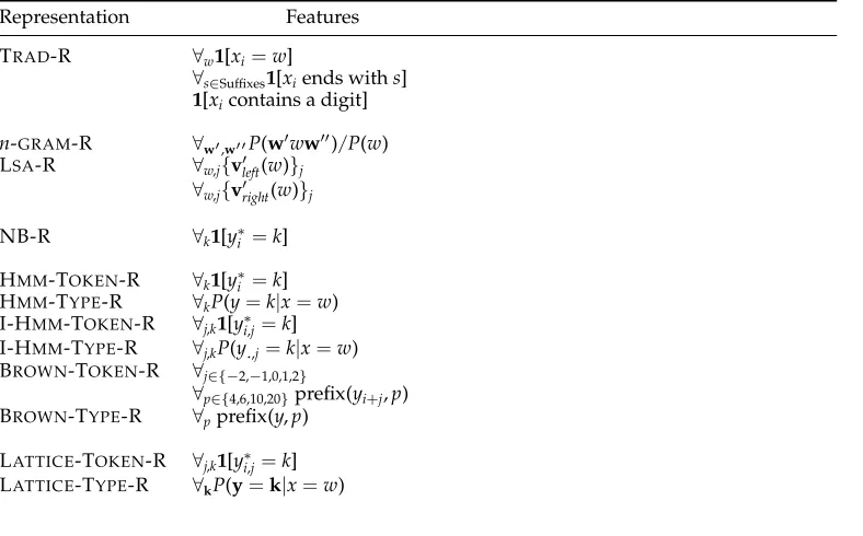
Figure 1

A graphical representation of the naive Bayes statistical language model. TheBandEare special dummy words for the beginning and end of the sentence.

of right context vectors and the set of left context vectors separately,1 _{to find}

reduced-rank versions v_right(w) andv_left(w), where each dimension represents a combination of several context word types. We then use each component of v_right(w) and v_left(w) as features. After experimenting with different choices for the number of dimensions to reduce our vectors to, we choose a value of 10 dimensions as the one that maximizes the performance of our supervised sequence labelers on held-out data. We call this model LSA-R.

3.3 A Context-Dependent Representation Using Naive Bayes

Then-GRAM-R and LSA-R representations always produce the same features F for a given word type w, regardless of the local context of a particular tokenxi=w. Our remaining representations are all context-dependent, in the sense that the features provided for tokenxi depend on the local context aroundxi. We begin with a statis-tical language model based on the Naive Bayes model with categorical latent states

S={1,. . .,K}. First, we form trigrams from our sentences. For each trigram, we form a separate Bayes net in which each token from the trigram is conditionally independent given the latent state. For tokensxi−1,xi, andxi+1, the probability of this trigram given

latent stateYi=yis given by:

P(xi−1,xi,xi+1|yi)=Pleft(xi−1|yi)Pmid(xi|yi)Pright(xi+1|yi) (6)

wherePleft,Pmid, andPrightare multinomial distributions conditioned on the latent state. The probability of a whole sentence is then given by the product of the probabilities of its trigrams. Figure 1 shows a graphical representation of this model. We train our models using standard expectation-maximization (Dempster, Laird, and Rubin 1977) with random initialization of the parameters.

Because our factorization of the sentence does not take into account the fact that the trigrams overlap, the resulting statistical language model is mass-deficient. Worse still, it is throwing away information from the dependencies among trigrams which might help make better clustering decisions. Nevertheless, this model closely mirrors many of the clustering algorithms used in previous approaches to representation learning for sequence labeling (Ushioda 1996; Miller, Guinness, and Zamanian 2004; Koo, Carreras,

and Collins 2008; Lin and Wu 2009; Ratinov and Roth 2009), and therefore serves as an important benchmark.

Given a naive Bayes statistical language model, we construct an NB-R representa-tion that produces|S|boolean featuresFs(xi) for each tokenxiand each possible latent states∈S:

Fs(xi)=

true ifs=arg max_s∈SP(xi−1,xi,xi+1|yi=s), false otherwise.

For a reasonable choice ofS(i.e.,|S| |V|), each feature should be observed often in a sufficiently large training data set. Therefore, compared with n-GRAM-R, NB-R

produces far fewer features. On the other hand, its features forxidepend not just on the contexts in whichxihas appeared in the statistical language model’s training data, but also on xi−1 and xi+1 in the current sentence. Furthermore, because the range of

the features is much more restrictive than real-valued features, it is less prone to data sparsity or variations across domains than real-valued features.

3.4 Context-Dependent, Structured Representations: The Hidden Markov Model

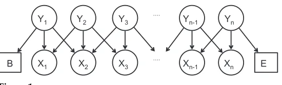
In previous work, we have implemented several representations based on hidden Markov models (Rabiner 1989), which we used for both sequential labeling (like POS tagging [Huang et al. 2011] and NP chunking [Huang and Yates 2009]) and IE (Downey, Schoenmackers, and Etzioni 2007). Figure 2 shows a graphical model of an HMM. An HMM is a generative probabilistic model that generates each word xi in the corpus conditioned on a latent variableyi. Eachyiin the model takes on integral values from 1 toK, and each one is generated by the latent variable for the preceding word,yi−1. The

joint distribution for a corpusx=(x1,. . .,xN) and a set of state vectorsy=(y1,. . .,yN) is given by: P(x,y)=_iP(xi|yi)P(yi|yi−1). Using expectation-maximization (EM)

(Dempster, Laird, and Rubin 1977), it is possible to estimate the distributions for

P(xi|yi) andP(yi|yi−1) from unlabeled data.

We construct two different representations from HMMs, one for sequence-labeling tasks and one for IE. For sequence labeling, we use the Viterbi algorithm to produce the optimal settingy∗of the latent states for a given sentencex, ory∗=argmax

y P(x,y). We

use the value ofy∗_i as a new feature forxi that represents a cluster of distributionally similar words. For IE, we require features for word types w, rather than tokens xi. Applying Bayes’ rule to the HMM parameters, we compute a distributionP(Y|x=w), whereYis a single latent node,xis a single token, andwis its word type. We then use each of theKvalues forP(Y=k|x=w), wherekranges from 1 toK, as features. This set

Figure 2

of features represents a “soft clustering” ofwintoKdifferent clusters. We refer to these representations as HMM-TOKEN-R and HMM-TYPE-R, respectively.

We also compare against a multi-layer variation of the HMM from our previous work (Huang and Yates 2010). This model trains an ensemble ofMindependent HMM models on the same corpus, initializing each one randomly. We can then use the Viterbi-optimal decoded latent state of each independent HMM model as a separate feature for a token, or the posterior distribution forP(Y|x=w) from each HMM as a separate set of features for each word type. We refer to this statistical language model as an I-HMM, and the representations as I-HMM-TOKEN-R and I-HMM-TYPE-R, respectively.

Finally, we compare against Brown clusters (Brown et al. 1992) as learned features. Although not traditionally described as such, Brown clustering involves constructing an HMM model in which each word type is restricted to having exactly one latent state that may generate it. Brown et al. describe a greedy agglomerative clustering algorithm for training this model on unlabeled text. Following Turian, Ratinov, and Bengio (2010), we use Percy Liang’s implementation of this algorithm for our comparison, and we test runs with 100, 320, 1,000 and 3,200 clusters. We use features from these clusters identical to Turian et al.’s.2 Turian et al. have shown that Brown clusters match or exceed the performance of neural network-based statistical language models in domain adaptation experiments for named-entity recognition, as well as in-domain experiments for NER and chunking.

Because HMM-based representations offer a small number of discrete states as features, they have a much greater potential to combat sparsity than don-gram mod-els. Furthermore, for token-based representations, these models can potentially handle polysemy better thann-gram statistical language models by providing different features in different contexts.

3.5 A Novel Lattice Statistical Language Model Representation

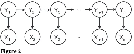
Our final statistical language model is a novel latent-variable statistical language model, called a Partial Lattice MRF (PL-MRF), with rich latent structure, shown in Figure 3. The model contains a lattice ofM×Nlatent states, where Nis the number of words in a sentence andMis the number of layers in the model. The dotted and solid lines in the figure together form a complete lattice of edges between these nodes; the PL-MRF uses only the solid edges. Formally, letc= N

2, whereNis the length of the sentence; leti

denote a position in the sentence, and letjdenote a layer in the lattice. Ifi<candjis odd, or ifjis even andi>c, we delete edges betweenyi,jandyi,j+1 from the complete

lattice. The same set of nodes remains, but the partial lattice contains fewer edges and paths between the nodes. A central “trunk” ati=cconnects all layers of the lattice, and branches from this trunk connect either to the branches in the layer above or the layer below (but not both).

The result is a model that retains most of the edges of the complete lattice, but unlike the complete lattice, it supports tractable inference. AsM,N→ ∞, five out of every six edges from the complete lattice appear in the PL-MRF. However, the PL-MRF makes the branches conditionally independent from one another, except through the trunk. For instance, the left branch between layers 1 and 2 ((y1,1,y1,2) and (y2,1,y2,2)) in

Figure 3 are disconnected; similarly, the right branch between layers 2 and 3 ((y4,2,y4,3) and (y5,2,y5,3)) are disconnected, except through the trunk and the observed nodes. As

y_4,1

y_3,1

y_4,2

y_3,2

y_4,3

y_3,3

y_4,4

y_3,4

y_4,5

y_3,5

x₁ y2,1

y_1,1

x₂ y2,2

y_1,2

x₃ y2,3

y_1,3

x₄ y2,4

y_1,4

x₅ y2,5

y_1,5

Figure 3

The PL-MRF model for a five-word sentence and a four-layer lattice. Dashed gray edges are part of a complete lattice, but not part of the PL-MRF.

a result, excluding the observed nodes, this model has a lowtree-widthof 2 (excluding observed nodes), and a variety of efficient dynamic programming and message-passing algorithms for training and inference can be readily applied (Bodlaender 1988). Our inference algorithm passes information from the branches inwards to the trunk, and then upward along the trunk, in time O(K4MN). In contrast, a fully connected lattice model has tree-width=min(M,N), making inference and learning intractable (Sutton, McCallum, and Rohanimanesh 2007), partly because of the difficulty in enumerating and summing over the exponentially-many configurationsyfor a givenx.

We can justify the choice of this model from a linguistic perspective as a way to capture the multi-dimensional nature of words. Linguists have long argued that words have many different features in a high dimensional space: They can be separately described by part of speech, gender, number, case, person, tense, voice, aspect, mass vs. count, and a host of semantic categories (agency, animate vs. inanimate, physical vs. abstract, etc.), to name a few (Sag, Wasow, and Bender 2003). In the PL-MRF, each layer of nodes is intended to represent some latent dimension of words.

We represent the probability distribution for PL-MRFs as log-linear models that decompose over cliques in the MRF graph. LetCliq(x,y) represent the set of all maximal cliques in the graph of the MRF model forxandy. Expressing the lattice model in log-linear form, we can write the marginal probabilityP(x) of a given sentencexas:

y

c∈Cliq(x,y)score(c,x,y)

x,y

c∈Cliq(x,y)score(c,x,y)

where score(c,x,y)=exp(θc·fc(xc,yc)). Our model includes parameters for transitions between two adjacent latent variables on layer j:θtrans_i,s,i+1,s,jforyi,j=sandyi+1,j=s. It also includes observation parameters for latent variables and tokens, as well as for pairs of adjacent latent variables in different layers and their tokens:θobs_i,j,s,wandθ_iobs_,j,s,j+1,s,wfor

As with our HMM models, we create two representations from PL-MRFs, one for tokens and one for types. For tokens, we decode the model to computey∗, the matrix of optimal latent state values for sentencex. For each layerjand and each possible latent state valuek, we add a boolean feature for token xi that is true iffy∗i,j=k. For word types, we compute distributions over the latent state space. Letybe a column vector of latent variables for word typew. For a PL-MRF model withMlayers of binary variables, there are 2M possible values for y. Our type representation computes a probability distribution over these 2M possible values, and uses each probability as a feature for

w.3_{We refer to these two representations as LATTICE-TOKEN-R and LATTICE-TYPE-R,}

respectively.

We train the PL-MRF using contrastive estimation (Smith and Eisner 2005), which iteratively optimizes the following objective function on a corpusX:

x∈X log

y

c∈Cliq(x,y)score(c,x,y)

x∈N(x),y

c∈Cliq(x,y)score(c,x,y)

(7)

whereN(x), the neighborhood ofx, indicates a set of perturbed variations of the original sentencex. Contrastive estimation seeks to move probability mass away from the per-turbed neighborhood sentences and onto the original sentence. We use a neighborhood function that includes all sentences which can be obtained from the original sentence by swapping the order of a consecutive pair of words. Training uses gradient descent over this non-convex objective function with a standard software package (Liu and Nocedal 1989) and converges to a local maximum or saddle point.

For tractability, we modify the training procedure to train the PL-MRF one layer at a time. Letθi represent the set of parameters relating to features of layeri, and let θ_¬i represent all other parameters. We fixθ¬0=0, and optimizeθ0 using contrastive

estimation. After convergence, we fixθ_¬1, and optimizeθ1, and so on. For training each

layer, we use a convergence threshold of 10−6on the objective function in Equation (7), and each layer typically converges in under 100 iterations.

4. Domain Adaptation with Learned Representations

We evaluate the representations described earlier on POS tagging and NP chunking tasks in a domain adaptation setting.

4.1 A Rich Problem Setting for Representation Learning

Existing supervised NLP systems are domain-dependent: There is a substantial drop in their performance when tested on data from a new domain. Domain adaptation is the task of overcoming this domain dependence. The aim is to build an accurate system for

3 This representation is only feasible for small numbers of layers, and in our experiments that require type representations, we usedM=10. For larger values ofM, other representations are also possible. We also experimented with a representation which included onlyMpossible values: For each layerl, we included

a target domain by training on labeled examples from a separate source domain. This problem is sometimes also calledtransfer learning(Raina et al. 2007).

Two of the challenges for NLP representations, sparsity and polysemy, are exacer-bated by domain adaptation. New domains come with new words and phrases that appear rarely (or even not at all) in the training domain, thus increasing problems with data sparsity. And even for words that do appear commonly in both domains, the contexts around the words will change from the training domain to the target domain. As a result, domain adaptation adds to the challenge of handling polysemous words, whose meaning depends on context.

In short, domain adaptation is a challenging setting for testing NLP representations. We now present several experiments testing our representations against state-of-the-art POS taggers in a variety of domain adaptation settings, showing that the learned representations surpass the previous state-of-the-art, without requiring any labeled data from the target domain.

4.2 Experimental Set-up

For domain adaptation, we test our representations on two sequence labeling tasks: POS tagging and chunking. To incorporate learned representation into our models, we follow this general procedure, although the details vary by experiment and are given in the following sections. First, we collect a set of unannotated text from both the training domain and test domain. Second, we learn representations on the unannotated text. We then automatically annotate both the training and test data with features from the learned representation. Finally, we train a supervised linear-chain CRF model on the annotated training set and apply it to the test set.

A linear-chain CRF is a Markov random field (Darroch, Lauritzen, and Speed 1980) in which the latent variables form a path with edges only between consecutive nodes in the path, and all latent variables are globally conditioned on the observations. LetXbe a random variable over data sequences, andZbe a random variable over corresponding label sequences. The conditional distribution over the label sequenceZgivenXhas the form

pθ(Z=z|X=x)∝exp

⎛

⎝

i

j

θ_jfj(zi−1,zi,x,i) ⎞

⎠ (8)

wherefj(zi−1,zi,x,i) is a real-valued feature function of the entire observation sequence and the labels at positionsiandi−1 in the label sequence, andθjis a parameter to be estimated from training data.

We use an open source CRF software package designed by Sunita Sarawagi to train and apply our CRF models.4 As is standard, we use two kinds of feature functions: transition and observation. Transition feature functions indicate, for each pair of labels

landl, whetherzi=landzi−1=l. Boolean observation feature functions indicate, for

each labelland each featuref provided by a representation, whetherzi=landxi has featuref. For each labelland each real-valued featurefin representationR, real-valued observation feature functions have valuef(x) ifzi=l, and are zero otherwise.

4.3 Domain Adaptation for POS Tagging

Our first experiment tests the performance of all the representations we introduced earlier on an English POS tagging task, trained on newswire text, to tag biomedical re-search literature. We follow Blitzer et al.’s experimental set-up. The labeled data consists of the WSJ portion of the Penn Treebank (Marcus, Marcinkiewicz, and Santorini 1993) as source domain data, and 561 labeled sentences (9,576 tokens) from the biomedical research literature database MEDLINE as target domain data (PennBioIE 2005). Fully 23% of the tokens in the labeled test text are never seen in the WSJ training data. The unlabeled data consists of the WSJ text plus 71,306 additional sentences of MEDLINE text (Blitzer, McDonald, and Pereira 2006). As a preprocessing step, we replacehapax legomena (defined as words that appear once in our unlabeled training data) with the special symbol*UNKNOWN*, and do the same for words in the labeled test sets that never appeared in any of our unlabeled training text.

For representations, we tested TRAD-R,n-GRAM-R, LSA-R, NB-R, HMM-TOKEN -R, I-HMM-TOKEN-R (between 2 and 8 layers), and LATTICE-TOKEN-R (8, 12, 16, and 20 layers). Each latent node in the I-HMMs had 80 possible values, creating 808 _≈1015 _{possible configurations of the eight-layer I-HMM for a single word. Each}

node in our PL-MRF is binary, creating a much smaller number (220_≈106_{) of possible}

configurations for each word in a 20-layer representation. To give then-gram model the largest training data set available, we trained it on the Web 1Tgram corpus (Brants and Franz 2006). We included the top 500 most commonn-grams for each word type, and then used mutual information on the training data to select the top 10,000 most relevantn-gram features for all word types, in order to keep the number of features manageable. We incorporatedn-gram features as binary values indicating whetherxi appeared with then-gram or not. For comparison, we also report on the performance of Brown clusters (100, 320, 1,000, and 3,200 possible clusters), following Turian, Ratinov, and Bengio (2010). Finally, we compare against Blitzer, McDonald, and Pereira (2006) SCL technique, described in Section 2.6, and the standard semi-supervised learning algorithm ASO (Ando and Zhang 2005), whose results on this task were previously reported by Blitzer, McDonald, and Pereira (2006).

Table 2 shows the results for the best variation of each kind of model—20 layers for the PL-MRF, 7 layers for the I-HMM, and 3,200 clusters for the Brown clustering. All statistical language model representations outperform the TRAD-R baseline.

In nearly all cases, learned representations significantly outperformed TRAD-R. The best representation, the 20-layer LATTICE-TOKEN-R, reduces error by 47% (35% on OOV) relative to the baseline TRAD-R, and by 44% (24% on out-of-vocabulary words (OOV)) relative to the benchmark SCL system. For comparison, this model achieved a 96.8% in-domain accuracy on Sections 22–24 of the Penn Treebank, about 0.5 percentage point shy of a state-of-the-art in-domain system with more sophisticated supervised learning (Shen, Satta, and Joshi 2007). The BROWN-TOKEN-R representation, which Turian, Ratinov, and Bengio (2010) demonstrated performed as well or better than a variety of neural network statistical language models as representations, achieved accuracies between the SCL system and the HMM-TOKEN-R. The WEB1T-n-GRAM-R, I-HMM-TOKEN-R, and LATTICE-TOKEN-R all performed quite close to one another, but the I-HMM-TOKEN-R and LATTICE-TOKEN-R were trained on many orders of magnitude less text. The LSA-R and NB-R outperformed the TRAD-R baseline but

not the SCL system. The n-GRAM-R, which was trained on the same text as the

other representations except the WEB1T-n-GRAM-R, performed far worse than the

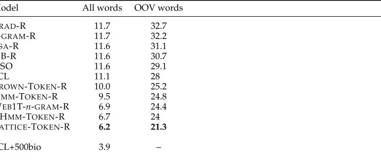
Table 2

Learned representations, and especially latent-variable statistical language model

representations, significantly outperform a traditional CRF system on domain adaptation for POS tagging. Percent error is shown for all words and out-of-vocabulary (OOV) words. The SCL+500bio system was given 500 labeled training sentences from the biomedical domain. 1.8% of tokens in the biomedical test set had POS tags like ‘HYPHENATED’, which are not part of the tagset for the training data, and were labeled incorrectly by all systems without access to labeled data from the biomedical domain. As a result, an error rate of 1.8 + 3.9 = 5.7 serves as a reasonable lower bound for a system that has never seen labeled examples from the biomedical domain.

Model All words OOV words

TRAD-R 11.7 32.7

n-GRAM-R 11.7 32.2

LSA-R 11.6 31.1

NB-R 11.6 30.7

ASO 11.6 29.1

SCL 11.1 28

BROWN-TOKEN-R 10.0 25.2

HMM-TOKEN-R 9.5 24.8

WEB1T-n-GRAM-R 6.9 24.4

I-HMM-TOKEN-R 6.7 24

LATTICE-TOKEN-R 6.2 21.3

SCL+500bio 3.9 –

The amount of unlabeled training data has a significant impact on the performance of these representations. This is apparent in the difference between WEB1T-n-GRAM -R andn-GRAM-R, but it is also true for our other representations. Figure 4 shows the accuracy of a representative subset of our taggers on words not seen in labeled training data, as we vary the amount of unlabeled training data available to the language

Figure 4

models. Performance grows steadily for all representations we measured, and none of the learning curves appears to have peaked. Furthermore, the margin between the more complex graphical models and the simplern-gram models grows with increasing amounts of training data.

4.3.1 Sparsity and Polysemy. We expected that statistical language model represen-tations would perform well in part because they provide meaningful features for sparse and polysemous words. For sparse tokens, these trends are already evident in the results in Table 2: Models that provide a constrained number of features, like HMM-based models, tend to outperform models that provide huge numbers of fea-tures (each of which, on average, is only sparsely observed in training data), like TRAD-R.

As for polysemy, HMM models significantly outperform naive Bayes models and then-GRAM-R. Then-GRAM-R’s features do not depend on a token type’s context at all, and the NB-R’s features depend only on the tokens immediately to the right and left of the current word. In contrast, the HMM takes into account all tokens in the surrounding sentence (although the strength of the dependence on more distant words decreases rapidly). Thus the performance of the HMM compared withn-GRAM-R and NB-R, as well as the performance of the LATTICE-TOKEN-R compared with the WEB1T-n -GRAM-R, suggests that representations that are sensitive to the context of a word

produce better features.

To test these effects more rigorously, we selected 109 polysemous word types from our test data, along with 296 non-polysemous word types. The set of polysemous word types was selected by filtering for words in our labeled data that had at least two POS tags that began with distinct letters (e.g., VBZ and NNS). An initial set of non-polysemous word types was selected by filtering for types that appeared with just one POS tag. We then manually inspected these initial selections to remove obvious cases of word types that were in fact polysemous within a single part-of-speech, such as “bank.” We further define sparse word types as those that appear five times or fewer in all of our unlabeled data, and we define non-sparse word types as those that appear at least 50 times in our unlabeled data. Table 3 shows our POS tagging results on the tokens of our labeled biomedical data with word types matching these four categories.

As expected, all of our statistical language models outperform the baseline by a larger margin on polysemous words than on non-polysemous words. The margin between graphical model representations and the WEB1T-n-GRAM-R model also

in-creases on polysemous words, except for the NB-R. The WEB1T-n-GRAM-R uses none of the local context to decide which features to provide, and the NB-R uses only the immediate left and right context, so both models ignore most of the context. In contrast, the remaining graphical models use Viterbi decoding to take into account all tokens in the surrounding sentence, which helps to explain their relative improvement over WEB1T-n-GRAM-R on polysemous words.

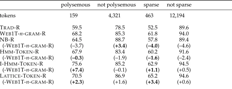
Table 3

Graphical models consistently outperformn-gram models by a larger margin on sparse words than not-sparse words, and by a larger margin on polysemous words than not-polysemous words. One exception is the NB-R, which performs worse relative to WEB1T-n-GRAM-R on polysemous words than non-polysemous words. For each graphical model representation, we show the difference in performance between that representation and WEB1T-n-GRAM-R in parentheses. For each representation, differences in accuracy on polysemous and non-polysemous subsets were statistically significant at p<0.01 using a two-tailed Fisher’s exact test. Likewise for performance on sparse vs. non-sparse categories.

polysemous not polysemous sparse not sparse

tokens 159 4,321 463 12,194

TRAD-R 59.5 78.5 52.5 89.6

WEB1T-n-GRAM-R 68.2 85.3 61.8 94.0

NB-R 64.5 88.7 57.8 89.4

(-WEB1T-n-GRAM-R) (–3.7) (+3.4) (–4.0) (–4.6)

HMM-TOKEN-R 67.9 83.4 60.2 91.6

(-WEB1T-n-GRAM-R) (–0.3) (–1.9) (–1.6) (–2.4)

I-HMM-TOKEN-R 75.6 85.2 62.9 94.5

(-WEB1T-n-GRAM-R) (+7.4) (–0.1) (+1.1) (+0.5)

LATTICE-TOKEN-R 70.5 86.9 65.2 94.6

(-WEB1T-n-GRAM-R) (+2.3) (+1.6) (+3.4) (+0.6)

on graphical models help address two key issues in building representations for POS tagging.

4.3.2 Domain Divergence.Besides sparsity and polysemy, Ben-David et al.’s (2007, 2010) theoretical analysis of domain adaptation shows that the distance between two domains under a representationRof the data is crucial for a good representation. We test their predictions using learned representations.

Ben-David et al.’s (2007, 2010) analysis depends on a particular notion of distance, thed1divergence, that is computationally intractable to calculate. For our analysis, we

resort instead to two different computationally efficient approximations of this measure. The first uses a more standard notion of distance: the Jensen-Shannon Divergence (dJS), a distance metric for probability distributions:

dJS(p||q)= 1₂

i

pilog _p

i mi

+qilog _q

i mi

wheremi= pi+q2 i.

Intuitively, we aim to measure the distance between two domains by measuring whether features appear more commonly in one domain than in the other. For instance, the biomedical domain is far from the newswire domain under the TRAD-R repre-sentation because word-based features likeprotein,gene, andpathwayappear far more commonly in the biomedical domain than the newswire domain. Likewise, bank and

president appear far more commonly in newswire text. Since thed1 distance is related

More formally, letSandTbe two domains, and letf be a feature5in representation

R—that is, a dimension of the image space of R. Let V be the set of possible values that f can take on. Let US be an unlabeled sample drawn from S, and likewise for UT. We first compute the relative frequencies of the different values off inR(US) and R(UT), and then computedJSbetween these empirical distributions. Letpf represent the empirical distribution overVestimated from observations of featurefinR(US), and let qf represent the same distribution estimated fromR(UT).

Definition 1

JS domain divergence for a feature or df(US,UT) is the domain divergence between domainsSandTunder featuref from representationR, and is given by

df(US,UT)=dJS(pf||qf)

For a multidimensional representation, we compute the full domain divergence as a weighted sum over the domain divergences for its features. Because individual features may vary in their relevance to a sequence-labeling task, we use weights to indicate their importance to the overall distance between the domains. We set the weightwf for featuref proportional to theL1norm of CRF parameters related tof in the trained

POS tagger. That is, letθ be the CRF parameters for our trained POS tagger, and let

θf ={θl,v|lbe the state forziandvbe the value forf}. We setwf =|| θf||1

||θ||1.

Definition 2

JS Domain Divergence ordR(US,UT), is the distance between domainsSandT under representationR, and is given by

dR(US,UT)=

f

wfdf(US,UT)

Blitzer (2008) uses a different notion of domain divergence to approximate the d1

divergence, which we also experimented with. He trains a CRF classifier on examples labeled with a tag indicating which domain the example was drawn from. We refer to this type of classifier as adomain classifier. Note that these should not be confused with our CRFs used for POS tagging, which take as input examples which are labeled with POS sequences. For the domain classifier, we tag every token from the WSJ domain as 0, and every token from the biomedical domain as 1. Blitzer then uses the accuracy of his domain classifier on a held-out test set as his measure of domain divergence. A high accuracy for the domain classifier indicates that the representation makes the two domains easy to separate, and thus high accuracy signifies a high domain divergence. To measure domain divergence using a domain classifier, we trained our representations on all of the unlabeled data for this task, as before. We then used 500 randomly sampled sentences from the WSJ domain, and 500 randomly sampled biomedical sentences, and labeled these with 0 for the WSJ data and 1 for the biomedical data. We measured the error rate of our domain-classifier CRF as the average error rate across folds when performing three-fold cross-validation on these 1,000 sentences.

0.88 0.89 0.9 0.91 0.92 0.93 0.94

0.32 0.37 0.42 0.47

Ta

rget Domain

Ta

gging A

ccuracy

Domain Divergence under the Representation

LATTICE-R

I-HMM-R

Trad-R

Ngram-R 1 HMM

7 HMMs

8 layer LATTICE 20 layer LATTICE

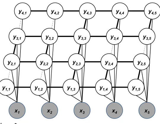
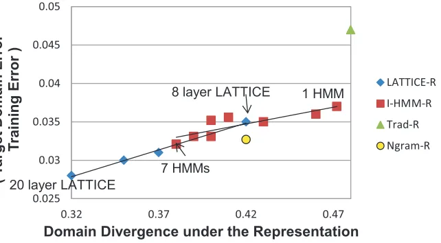
Figure 5

Target-domain POS tagging accuracy for a model developed using a representationRcorrelates strongly with lower JS domain divergence between WSJ and biomedical text under each representationR. The correlation coefficientsr2_{for the linear regressions drawn in the}

figure are both greater than 0.97.

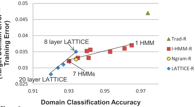
Figure 5 plots the accuracies and JS domain divergences for our POS taggers. Figure 6 shows the difference between target-domain error and source-domain error as a function of JS domain divergence. Figures 7 and 8 show the same information, except that the x axis plots the accuracy of a domain classifier as the way of mea-suring domain divergence. These results give empirical support to Ben-David et al.’s (2007, 2010) theoretical analysis: Smaller domain divergence—whether measured by JS domain divergence or by the accuracy of a domain classifier—correlates strongly with better target-domain accuracy. Furthermore, smaller domain divergence correlates strongly with a smaller difference in the accuracy of the taggers on the source and target domains.

Figure 6

0.88 0.89 0.9 0.91 0.92 0.93 0.94 0.95

0.91 0.92 0.93 0.94 0.95 0.96 0.97 0.98

Ta

rget Domain

Ta

gging A

ccuracy

Domain Classification Accuracy

Trad Rep

I-HMM

Ngram

PL-MRF 1 HMM

7 HMMs 20 layer PL-MRF

8 layer PL-MRF

Figure 7

Target-domain tagging accuracy decreases with the accuracy of a CRF domain classifier. Intuitively, this means that training data from a source domain is less helpful for tagging in a target domain when source-domain data is easy to distinguish from target-domain data.

Figure 8

Better domain classification correlates with a larger difference between target-domain error and source-domain error.

Although both the JS domain divergence and the domain classifier provide only approximations of the d1 metric for domain divergence, they agree very strongly:

In both cases, the LATTICE-TOKEN-R representations had the lowest domain diver-gence, followed by the I-HMM-TOKEN-R representations, followed by TRAD-R, with

n-GRAM-R somewhere between LATTICE-TOKEN-R and I-HMM-TOKEN-R. The main difference between the two metrics appears to be that the JS domain divergence gives a greater domain divergence to the eight-layer LATTICE-TOKEN-R model and the

The domain divergences of all models, using both techniques for measuring diver-gence, remain significantly far from zero, even under the best representation. As a result, there is ample room to experiment with even less-divergent representations of the two domains, to see if they might yield ever-increasing target-domain accuracies. Note that this is not simply a matter of adding more layers to the layered models. The I-HMM

-TOKEN-R model performed best with seven layers, and the eight-layer representation

had about the same accuracy and domain divergence as the five-layer model. This may be explained by the fact that the I-HMM layers are trained independently, and so additional layers may be duplicating other ones, and causing the supervised classifier to overfit. But it also shows that our current methodology has no built-in technique for constraining the domain divergence in our representations—the decrease in domain divergence from our more sophisticated representations is a coincidental byproduct of our training methodology, but there is no guarantee that our current mechanisms will continue to decrease domain divergence simply by increasing the number of layers. An important consideration for future research is to devise explicit learning mechanisms that guide representations towards smaller domain divergences.

4.4 Domain Adaptation for Noun-Phrase Chunking and Chinese POS Tagging

We test the generality of our representations by using them for other tasks, domains, and languages. Here, we report on further sequence-labeling tasks in a domain adaptation setting: noun phrase chunking for adaptation from news text to biochemistry journals, and POS tagging in Mandarin for a variety of domains. In the next section, we describe the use of our representations in a weakly supervised information extraction task.

For chunking, the training set consists of the CoNLL 2000 shared task data for source-domain labeled data (Sections 15–18 of the WSJ portion of the Penn Treebank, labeled with chunk tags) (Tjong, Sang, and Buchholz 2000). For test data, we used biochemistry journal data from the Open American National Corpus6 (OANC). One of the authors manually labeled 198 randomly selected sentences (5,361 tokens) from the OANC biochemistry text with noun-phrase chunk information.7We focus on noun phrase chunks because they are relatively easy to annotate manually, but contain a large variety of open-class words that vary from domain to domain. The labeled training set consists of 8,936 sentences and 211,726 tokens. Twenty-three percent of chunks in the test set begin with an OOV word (especially adjective-noun constructions like “aqueous formation” and “angular recess”), and 29% begin with a word seen at most twice in training data; we refer to these as OOV chunks and rare chunks. For our unlabeled data, we use 15,000 sentences (358,000 tokens; Sections 13–19) of the Penn Treebank and 45,000 sentences (1,083,000 tokens) from the OANC’s biochemistry section. We tested TRAD-R (augmented with features for automatically generated POS tags), LSA-R,

n-GRAM-R, NB-R, HMM-TOKEN-R, I-HMM-TOKEN-R (7 layers, which performed best for POS tagging) and LATTICE-TOKEN-R (20 layers) representations.

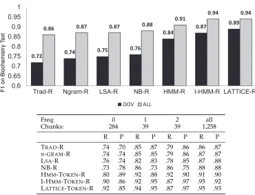
Figure 9 shows our NP chunking results for this domain adaptation task. The performance improvements for the HMM-based chunkers are impressive: LATTICE -TOKEN-R reduces error by 57% with respect to TRAD-R, and comes close to state-of-the-art results for chunking on newswire text. The results suggest that this representation allows the CRF to generalize almost as well to out-of-domain text as in-domain text.

6 Available fromhttp://www.anc.org/OANC/.

F1

on

Biochemistr

y

T

e

xt

0.72 0.74 0.75

0.76

0.84 0.87

0.89

0.86 0.87 0.87 0.88

0.91 0.94 0.94

0.6 0.65 0.7 0.75 0.8 0.85 0.9 0.95 1

Trad-R Ngram-R LSA-R NB-R HMM-R I-HMM-R LATTICE-R

OOV ALL

Freq: 0 1 2 all

Chunks: 284 39 39 1,258

R P R P R P R P

TRAD-R .74 .70 .85 .87 .79 .86 .86 .87

n-GRAM-R .74 .74 .85 .85 .79 .86 .87 .87

LSA-R .76 .74 .82 .83 .78 .85 .87 .88

NB-R .73 .78 .86 .73 .86 .75 .88 .88

HMM-TOKEN-R .80 .89 .92 .88 .92 .90 .91 .90 I-HMM-TOKEN-R .90 .86 .92 .95 .87 .97 .95 .92 LATTICE-TOKEN-R .92 .85 .94 .95 .87 .97 .95 .93

Figure 9

On biomedical journal data from the OANC, our best NP chunker outperforms the baseline CRF chunker by 0.17 F1 on chunks that begin with OOV words, and by 0.08 on all chunks. The table shows performance breakdowns (recall and precision) for chunks whose first word has frequency 0, 1, and 2 in training data, and the number of chunks in test data that fall into each of these categories.

Improvements are greatest on OOV and rare chunks, where LATTICE-TOKEN-R made absolute improvements over TRAD-R by 0.17 and 0.09 F1, respectively. Improvements for the single-layer HMM-TOKEN-R were smaller but still significant: 36% relative re-duction in error overall, and 32% for OOV chunks.

The improved performance from our HMM-based chunker caused us to wonder how well the chunker could work without some of its other features. We removed all tag features and orthographic features and all features for word types that appear fewer than 20 times in training. This chunker still achieves 0.91 F1 on OANC data, and 0.93 F1 on WSJ data (Section 20), outperforming the TRAD-R system in both cases. It has only 20% as many features as the baseline chunker, greatly improving its training time. Thus these features are more valuable to the chunker than features from automatically produced tags and features for all but the most common words.