Discriminative Word Alignment by Linear Modeling

Linear Modeling

Yang Liu

Institute of Computing Technology Chinese Academy of Sciences

Qun Liu

Institute of Computing Technology Chinese Academy of Sciences

Shouxun Lin

Institute of Computing Technology Chinese Academy of Sciences

Word alignment plays an important role in many NLP tasks as it indicates the correspondence between words in a parallel text. Although widely used to align large bilingual corpora, gen-erative models are hard to extend to incorporate arbitrary useful linguistic information. This article presents a discriminative framework for word alignment based on a linear model. Within this framework, all knowledge sources are treated as feature functions, which depend on a source language sentence, a target language sentence, and the alignment between them. We describe a number of features that could produce symmetric alignments. Our model is easy to extend and can be optimized with respect to evaluation metrics directly. The model achieves state-of-the-art alignment quality on three word alignment shared tasks for five language pairs with varying divergence and richness of resources. We further show that our approach improves translation performance for various statistical machine translation systems.

1. Introduction

Word alignment, which can be defined as an object for indicating the corresponding words in a parallel text, was first introduced as an intermediate result of statistical machine translation (Brown et al. 1993).

Consider the following Chinese sentence and its English translation:

dd ddd dddd dd d dd

Zhongguo jianzhuye duiwaikaifang chengxian xin geju

The opening of China’s construction industry to the outside presents a new structure

∗Key Laboratory of Intelligent Information Processing, Institute of Computing Technology, Chinese Academy of Sciences, No. 6 Kexueyuan South Road, Haidian District, P.O. Box 2704, Beijing 100190, China. E-mail:{yliu, liuqun, sxlin}@ict.ac.cn.

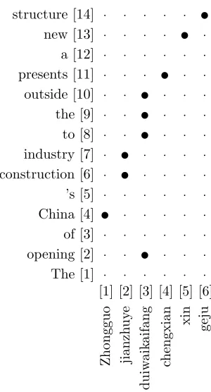
The Chinese word Zhongguo is aligned to the English word China because they are translations of one another. Similarly, the Chinese word xin is aligned to the English wordnew. These connections are not necessarily one-to-one. For example, one Chinese wordjianzhuyecorresponds to two English wordsconstruction industry. In addition, the English words (e.g., opening ... to the outside) connected to a Chinese word (e.g., dui-waikaifang) could be discontinuous. Figure 1 shows an alignment for this sentence pair. The Chinese and English words are listed horizontally and vertically, respectively. They are numbered to facilitate identification. The dark points indicate the correspondence between the words in two languages. The goal of word alignment is to identify such correspondences in a parallel text.

Word alignment plays an important role in many NLP tasks. In statistical machine translation, word-aligned corpora serve as an excellent source for translation-related knowledge. The estimation of translation model parameters usually relies heavily on word-aligned corpora, not only for phrase-based and hierarchical phrase-based models (Koehn, Och, and Marcu 2003; Och and Ney 2004; Chiang 2005, 2007), but also for syntax-based models (Quirk, Menezes, and Cherry 2005; Galley et al. 2006; Liu, Liu, and Lin 2006; Marcu et al. 2006). Besides machine translation, many applications for word-aligned corpora have been suggested, including machine-assisted translation,

Figure 1

translation assessment and critiquing tools, text generation, bilingual lexigraphy, and word sense disambiguation.

Various methods have been proposed for finding word alignments between parallel texts. Among them, generative alignment models (Brown et al. 1993; Vogel and Ney 1996) have been widely used to produce word alignments for large bilingual corpora. Describing the relationship of a bilingual sentence pair, a generative model treats word alignment as a hidden process and maximizes the likelihood of a training corpus using the expectation maximization (EM) algorithm. After the maximization process is com-plete, the unknown model parameters are determined and the word alignments are set to the maximum posterior predictions of the model.

However, one drawback of generative models is that they are hard to extend. Gen-erative models usually impose strong independence assumptions between sub-models, making it very difficult to incorporate arbitrary features explicitly. For example, when considering whether to align two words, generative models cannot include information about lexical and syntactic features such as part of speech and orthographic similarity in an easy way. Such features would allow for more effective use of sparse data and result in a model that is more robust in the presence of unseen words. Extending a generative model requires that the interdependence of information sources be modeled explicitly, which often makes the resulting system quite complex.

In this article, we introduce a discriminative framework for word alignment based on the linear modeling approach. Within this framework, we treat all knowledge sources as feature functions that depend on a source sentence, a target sentence, and the alignment between them. Each feature function is associated with a feature weight. The linear combination of features gives an overall score to each candidate alignment. The best alignment is the one with the highest overall score. A linear model not only allows for easy integration of new features, but also admits optimiz-ing feature weights directly with respect to evaluation metrics. Experimental results show that our approach improves both alignment quality and translation performance significantly.

This article is organized as follows. Section 2 gives a formal description of our model. We show how to train feature weights by taking evaluation metrics into account and how to find the most probable alignment in an exponential search space efficiently. Section 3 describes a number of features used in our experiments, focusing on the features that produce symmetric alignments. In Section 4, we evaluate our model in both alignment and translation tasks. Section 5 reviews previous work related to our approach and the article closes with a conclusion in Section 6.

2. Approach

2.1 The Model

Given a source language sentencef=f1,. . .,fj,. . .,fJand a target language sentencee= e1,. . .,ei,. . .,eI, we define alinkl=(j,i) to exist iffjandeiare translations (or part of a translation) of one another. Then, analignmentis defined as a subset of the Cartesian product of the word positions:

We propose a linear alignment model:

score(f,e,a)=

M

m=1

λmhm(f,e,a) (2)

wherehm(f,e,a) is afeature functionandλmis its associatedfeature weight. The linear combination of features gives an overall scorescore(f,e,a) to each candidate alignment afor a given sentence pairf,e.

2.2 Training

To achieve good alignment quality, it is essential to find a good set of feature weights

λM₁ . Before discussing how to trainλM₁ , we first describe two evaluation metrics that measure alignment quality, because we will optimizeλM₁ with respect to them directly.

2.2.1 Evaluation Metrics. The first metric isalignment error rate (AER), proposed by Och and Ney (2003). AER has been used as official evaluation criterion in most word alignment shared tasks. Och and Ney define two kinds of links in hand-aligned align-ments: sure links for alignments that are unambiguous and possible links for ambiguous alignments. Sure links usually connect content words such as Zhongguo and China. In contrast, possible links often align words within idiomatic expressions and free translations.

An AER score is given by

AER(S,P,A)=1− |A∩S|+|A∩P|

|A|+|S| (3)

whereSis a set of sure links in a reference alignment that is hand-aligned by human experts, P is a set of possible links in the reference alignment, and Ais a candidate alignment. Note thatSis a subset ofP:S⊆P. The lower the AER score is, the better the alignment quality is.

Although widely used, AER has been criticized for correlating poorly with transla-tion quality (Ayan and Dorr 2006a; Fraser and Marcu 2007b). In other words, lower AER scores do not necessarily lead to better translation quality.1 _{Fraser and Marcu (2007b)}

argue that reference alignments should consist of only sure links. They propose a new measure called thebalanced F-measure:

precision(S,A)= |A∩S|

|S| (4)

recall(S,A)= |A∩S|

|A| (5)

F-measure(S,α,A)= 1

α

precision(S,A)+recall(1−αS,A)

(6)

where α is a parameter that sets the trade-off between precision and recall. Higher F-measure means better alignment quality. Obviously, α less than 0.5 weights recall higher, whereasαgreater than 0.5 weights precision higher.

We use both AER and F-measure in our experiments. AER is used in experiments evaluating alignment quality (Section 4.1) and F-measure is used in experiments evalu-ating translation performance (Section 4.2).

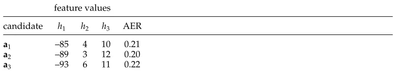
2.2.2 Minimum Error Rate Training.Suppose we have three candidate alignments:a1,a2,

anda3. Their AER scores are 0.21, 0.20, and 0.22, respectively. Therefore,a2is the best

candidate alignment,a1is the second best, anda3is the third best. We use three features

to score each candidate. Table 1 lists the feature values for each candidate.

If the set of feature weights is{1.0, 1.0, 1.0}, the model scores (see Equation (2)) of the three candidates are−71,−74, and−76, respectively. Whereas reference alignment considersa2as the best candidate,a1has the maximal model score. This is undesirable

because the model fails to agree with the reference. If we change the feature weights to{1.0,−2.0, 2.0}, the model scores become−73,−71, and−83, respectively. Now, the model choosesa2as the best candidate correctly.

If a set of feature weights manages to make model predictions agree with refer-ence alignments in training examples, we would expect the model to achieve good alignment quality on unseen data as well. To do this, we adopt the minimum er-ror rate training (MERT) algorithm proposed by Och (2003) to find feature weights that minimize AER or maximize F-measure on a representative hand-aligned training corpus.

Given a reference alignment r and a candidate alignment a, we use a loss func-tionE(r,a) to measure alignment performance. Note that E(r,a) can be either AER or 1−F-measure. Given a bilingual corpusfS₁,eS₁with a reference alignmentrsand a set ofKdifferent candidate alignmentsCs={as,1. . .as,K}for each sentence pairfs,es, our goal is to find a set of feature weights ˆλM₁ that minimizes the overall loss on the training corpus:

ˆ

λM₁ =argmin λM

1

S

s=1

E(rs, ˆa(fs,es;λM1 ))

(7)

=argmin λM

1

S

s=1

K

k=1

E(rs,as,k)δ(ˆa(fs,es;λM1 ),as,k)

(8)

Table 1

Example feature values and alignment error rates.

feature values

candidate h1 h2 h3 AER

a1 –85 4 10 0.21

a2 –89 3 12 0.20

where ˆa(fs,es;λM1 ) is the best candidate alignment produced by the linear model:

ˆ

a(fs,es;λM₁ )=argmax a

M

m=1

λmhm(fs,es,a)

(9)

The basic idea of MERT is to optimize only one parameter (i.e., feature weight) each time and keep all other parameters fixed. This process runs iteratively over M

parameters until the overall loss on the training corpus does not decrease.

Formally, suppose we tune a parameter and keep the otherM−1 parameters fixed; each candidate alignment corresponds to a line in the plane withγas the independent variable:

γ·μ(f,e,a)+σ(f,e,a) (10)

where γ denotes the parameter being tuned (i.e., λm) and μ(f,e,a) and σ(f,e,a) are constants with respect toγ:

μ(f,e,a)=hm(f,e,a) (11)

σ(f,e,a)=

M

m=1,m=m

λ_mhm(f,e,a) (12)

The set of candidates inCs defines a set of lines. For example, given the candidate alignments in Table 1, suppose we only tuneλ₂and keepλ₁andλ₃fixed with an initial set of parameters {1.0, 1.0, 1.0}. According to Equation (10), a1 corresponds to a line

4γ−75,a2corresponds to a line 3γ−77, anda3corresponds to a line 6γ−82.

The decision rule in Equation (9) states that ˆa is the line with the highest model score for a givenγ. The selection ofγfor each sentence pair ultimately determines the loss atγ. How do we find values ofγthat could generate different loss values?

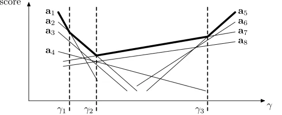
As the loss can only change if we move to aγ where the highest line is different than before, Och (2003) suggests only evaluating the loss at values in between the intersections that line the top surface of the cluster of lines. Figure 2 demonstrates eight

Figure 2

Candidate alignments in dimensionγand the critical intersections. Each candidate alignment is represented as a line.γ1,γ2, andγ3are critical intersections where the best candidate ˆa

candidate alignments. The sequence of the topmost line segments highlighted in bold constitutes an upper envelope, which indicates the best candidate alignments the model predicts with various values of γ. Instead of computing all possible K2 _{intersections}

between the lines inCs, we just need to find thecritical intersectionswhere the topmost line changes. In Figure 2,γ1,γ2, andγ3are critical intersections. In the interval (−∞,γ1],

a1has the highest score. Similarly, the best candidates area2for (γ1,γ2],a7 for (γ2,γ3],

anda5 for (γ3,+∞), respectively. The optimal ˆγcan be found by collecting all critical

intersections on the training corpus and choosing oneγthat results in the minimal loss value. Please refer to Och (2003) for more details.

2.3 Search

Given a source language sentencefand a target language sentencee, we try to find the best candidate alignment with the highest model score:

ˆ

a=argmax a

score(f,e,a)

(13)

=argmax a

M

m=1

λ_mhm(f,e,a)

(14)

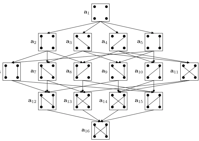
To do this, we begin with an empty alignment and keep adding new links until the model score of the current alignment does not increase. Figure 3 illustrates this search process. Given a source language sentencef1f2 and a target language sentence

e1e2, the initial alignmenta1 is empty (i.e., all words are unaligned). Then, we obtain a

new alignmenta2by adding a link (1, 1) toa1. Similarly, the addition of (1, 2) toa1leads

toa3.a2anda3can be further extended to produce more alignments.

Graphically speaking, the search space of a sentence pair can be organized as a directed acyclic graph. Each node in the graph is a candidate alignment and each edge corresponds to a link. We say that alignments that have the same number of links constitute a level. There are 2J×I possible nodes and J×I+1 levels in a graph. In Figure 3,a2,a3,a4, anda5 belong to the same level because they all contain one link.

The maximum level width is given byJJ××₂II

. In Figure 3, the maximal level width is

₄ 2

= 6. Our goal is to find the node with the highest model score in a search graph. As the search space of word alignment is exponential (although enumerable), it is computationally prohibitive to explore all the graph. Instead, we can search efficiently in a greedy way. In Figure 3, starting froma1, we add single links toa1and obtain four

new alignments:a2,a3,a4, anda5. We retain the best new alignment that has a higher

score thana1, saya3, and discard the others. Then, we add single links toa3and obtain

three new alignments:a7,a9, anda11. After choosinga9as the current best alignment, the

next candidates area12anda14. Suppose the model scores of botha12anda14are lower

than that ofa9. We terminate the search process and choose a9 as the best candidate

alignment.

During this search process, we expect that the addition of a single link l to the current best alignmentawill result in a new alignmenta∪ {l}with a higher score:

Figure 3

Search space of a sentence pair:f1f2ande1e2. Each node in the directed graph is a candidate alignment and each edge denotes a transition between two nodes by adding a link.

that is

M

m=1

λm

hm(f,e,a∪ {l})−hm(f,e,a)

>0 (16)

As a result, we can remove most of the computational overhead by calculating only the difference of scores instead of the scores themselves. The difference of alignment scores with the addition of a link, which we refer to as alink gain, is defined as

G(f,e,a,l)=

M

m=1

λ_mgm(f,e,a,l) (17)

wheregm(f,e,a,l) is afeature gain, which is the incremental feature value after adding a linklto the current alignmenta:

gm(f,e,a,l)=hm(f,e,a∪ {l})−hm(f,e,a) (18)

In our experiments, we use a beam search algorithm that is more general than the above greedy algorithm. In the greedy algorithm, we retain at most one candidate in each level of the space graph while traversing top-down. In the beam search algorithm, we retain at mostbcandidates at each level.

Algorithm 1A beam search algorithm for word alignment 1: procedureALIGN(f,e)

2: open← ∅ a list of active alignments

3: N ← ∅ n-best list

4: a← ∅ begin with an empty alignment

5: ADD(open,a,β,b) initialize the list

6: whileopen=∅do

7: closed← ∅ a list of promising alignments

8: for all a∈opendo

9: for alll∈J×I−a do enumerate all possible new links

10: a←a∪ {l} produce a new alignment

11: g←GAIN(f,e,a,l) compute the link gain

12: ifg>0then ensure that the score will increase

13: ADD(closed,a,β,b) update promising alignments

14: end if

15: ADD(N,a, 0,n) updaten-best list

16: end for

17: end for

18: open←closed update active alignments

19: end while

20: returnN returnn-best list

21: end procedure

active alignmentsopen(line 2) and ann-best listN (line 3). The aligning process begins with an empty alignmenta(line 4) and the procedure ADD(open,a,β,b) addsatoopen. The procedure prunes the search space by discarding any alignment that has a score worse than:

1. βmultiplied with the best score in the list, or 2. the score ofb-th best alignment in the list.

For each iteration (line 6), we use a list closedto store promising alignments that have higher scores than the current alignment. For every possible link l (line 9), we produce a new alignment a (line 10) and calculate the link gain G by calling the procedure GAIN(f,e,a,l). Ifahas a higher score (line 12), it is added toclosed(line 13). We also updateN to keep the topnalignments explored during the search (line 15). The

n-best list will be used in training feature weights by MERT. This process iterates until there are no promising alignments. The theoretical running time of this algorithm isO(bJ2I2).

3. Feature Functions

and Lin 2005). Another way is to treat each sub-model of a generative model as a feature (Fraser and Marcu 2006). In either case, a generative model can be regarded as a special case of a discriminative model where all feature weights are one. A detailed discussion of the treatment of the IBM models as features can be found in Appendix B.

One major drawback of the IBM models is asymmetry. They are restricted such that each source word is assigned to exactly one target word. This is not the case for many language pairs. For example, in our running example, one Chinese wordjianzhuye cor-responds to two English wordsconstruction industry. As a result, our linear model will produce only one-to-one alignments if the IBM models in two translation directions (i.e., source-to-target and target-to-source) are both used. Although some authors would use the one-to-one assumption to simplify the modeling problem (Melamed 2000; Taskar, Lacoste-Julien, and Klein 2005), many translation phenomena cannot be handled and the recall cannot reach 100% in principle.

A more general way is to model alignment as an arbitrary relation between source and target language word positions. As our linear model is capable of including many overlapping features regardless of their interdependencies, it is easy to add features that characterize symmetric alignments. In the following subsections, we will introduce a number of symmetric features used in our experiments.

3.1 Translation Probability Product

To determine the correspondence of words in two languages, word-to-word translation probabilities are always the most important knowledge source. To model a symmetric alignment, a straightforward way is to compute the product of the translation probabil-ities of each link in two directions.

For example, suppose that there is an alignment {(1, 2)} for a source language sentence f1f2 and a target language sentence e1e2; the translation probability

prod-uct is

t(e2|f1)×t(f1|e2)

wheret(e|f) is the probability thatf is translated toeandt(f|e) is the probability thate

is translated tof, respectively.

Unfortunately, the underlying model is biased: The more links added, the smaller the product will be. For example, if we add a link (2, 2) to the current alignment and obtain a new alignment{(1, 2), (2, 2)}, the resulting product will decrease after being multiplied witht(e2|f2)×t(f2|e2):

t(e2|f1)×t(f1|e2)×t(e2|f2)×t(f2|e2)

The problem results from the absence of emptycepts. Following Brown et al. (1993), a cept in an alignment is either a single source word or it is empty. They assign cepts to positions in the source sentence and reserve position zero for the empty cept. All unaligned target words are assumed to be “aligned” to the empty cept. For example, in the current example alignment {(1, 2)}, the unaligned target worde1 is said to be

“aligned” to the empty cept f0. As our model is symmetric, we usef0 to denote the

empty cept on the source side and usee0 to denote the empty cept on the target side,

If we take empty cepts into account, the product for{(1, 2)}can be rewritten as

t(e2|f1)×t(f1|e2)×t(e1|f0)×t(f2|e0)

Similarly, the product for{(1, 2), (2, 2)}now becomes

t(e2|f1)×t(f1|e2)×t(e2|f2)×t(f2|e2)×t(e1|f0)

Note that after adding the link (2, 2), the new product still has more factors than the old product. However, the new product is not necessarily always smaller than the old one. In this case, the new product divided by the old product is

t(e2|f2)×t(f2|e2)

t(f2|e0)

Whether a new product increases or not depends on actual translation probabilities.2

Depending on whether they are aligned or not, we divide the words in a sentence pair into two categories:alignedandunaligned. For each aligned word, we use trans-lation probabilities conditioned on its counterpart in two directions (i.e., t(ei|fj) and t(fj|ei)). For each unaligned word, we use translation probabilities conditioned on empty cepts on the other side in two directions (i.e.,t(ei|f0) andt(fj|e0)).

Formally, the feature function for translation probability product is given by3

htpp(f,e,a)=

(j,i)∈a

logt(ei|fj)

+logt(fj|ei)

+

J

j=1

logδ(ψ_j, 0)×t(fj|e0)+1−δ(ψj, 0)

+

I

i=1

logδ(φi, 0)×t(ei|f0)+1−δ(φi, 0)

(19)

whereδ(x,y) is the Kronecker function, which is 1 ifx=yand 0 otherwise. We define thefertilityof a source wordfjas the number of aligned target words:

ψj=

(j,i)∈a

δ(j,j) (20)

2 Even though we take empty cepts into account, the bias problem still exists because the product will decrease by adding new links if there are no unaligned words. For example, the product will go down if we further add a link (1, 1) to{(1, 2), (2, 2)}as all source words are aligned. This might not be a bad bias because reference alignments usually do not have all words aligned and contain too many links. Although translation probability product is degenerate as a generative model, the bias problem can be alleviated when this feature is combined with other features such as link count (see Section 3.8). 3 We use the logarithmic form of translation probability product to avoid manipulating very small

Table 2

Calculating feature values of translation probability product for a source sentencef1f2and a target sentencee1e2.

alignment feature value

{} logt(e1|f0)·t(e2|f0)·t(f1|e0)·t(f2|e0) {(1, 2)} logt(e1|f0)·t(e2|f1)·t(f1|e2)·t(f2|e0) {(1, 2), (2, 2)} logt(e1|f0)·t(e2|f1)·t(e2|f2)·t(f1|e2)·t(f2|e2)

Similarly, the fertility of a target wordeiis the number of aligned source words:

φi=

(j,i)∈a

δ(i,i) (21)

For example, as only one English wordChinais aligned to the first Chinese word

Zhongguo in Figure 1, the fertility ofZhongguo isψ₁ =1. Similarly, the fertility of the third Chinese word duiwaikaifang is ψ₃ =4 because there are four aligned English words. The fertility of the first English wordTheisφ1=0. Obviously, the words with

zero fertilities (e.g.,The,’s, andain Figure 1) are unaligned.

In Equation (19), the first term calculates the product of aligned words, the second term deals with unaligned source words, and the third term deals with unaligned target words. Table 2 shows the feature values for some word alignments.

For efficiency, we need to calculate the difference of feature values instead of the values themselves, which we call feature gain (see Equation (18)). The feature gain for translation probability product is4

gtpp(f,e,a,j,i)=log

t(ei|fj)

+logt(fj|ei)

−

logδ(ψj, 0)×t(fj|e0)+1−δ(ψj, 0)

−

logδ(φ_i, 0)×t(ei|f0)+1−δ(φi, 0)

(22)

whereψ_jandφ_iare the fertilities before adding the link (j,i).

Although this feature is symmetric, we obtain the translation probabilitiest(f|e) and

t(e|f) by training the IBM models using GIZA++ (Och and Ney 2003). 3.2 Exact Match

Motivated by the fact that proper names (e.g.,IBM) or specialized terms (e.g.,DNA) are often the same in both languages, Taskar, Lacoste-Julien, and Klein (2005) use a feature that sums up the number of words linked to identical words. We adopt this exact match feature in our model:

hem(f,e,a)=

(j,i)∈a

δ(fj,ei) (23)

gem(f,e,a,j,i)=δ(fj,ei) (24)

3.3 Cross Count

Due to the diversity of natural languages, word orders between two languages are usu-ally different. For example, subject-verb-object (SVO) languages such as Chinese and English often put an object after a verb while subject-object-verb (SOV) languages such as Japanese and Turkish often put an object before a verb. Even between SVO languages such as Chinese and English, word orders could be quite different too. In Figure 1, while Zhongguo is the first Chinese word, its counterpart Chinais the fourth English word. Meanwhile, the third Chinese wordduiwaikaifangafterZhongguois aligned to the second English wordopeningbeforeChina. We say that there is acrossbetween the two links (1, 4) and (3, 2) because (1−3)×(4−2)<0. In Figure 1, there is only one cross. As a result, we could use the number of crosses in alignments to capture the divergence of word orders between two languages.

Formally, the cross count feature function is given by

hcc(f,e,a)=

(j,i)∈a

(j,i)∈a

(j−j)×(i−i)<0 (25)

gcc(f,e,a,j,i)=

(j,i)∈a

(j−j)×(i−i)<0 (26)

where expr is an indicator function that takes a boolean expression expr as the argument:

expr=

1 ifexpris true

0 otherwise (27)

3.4 Neighbor Count

Moore (2005) finds that word alignments between closely related languages tend to be approximately monotonic. Even for distantly related languages, the number of crossing links is far less than chance since phrases tend to be translated as contiguous chunks. In Figure 1, the dark points are positioned approximately in parallel with the diagonal line, indicating that the alignment is approximately monotonic.

To capture such monotonicity, we follow Lacoste-Julien et al. (2006) to encourage strictly monotonic alignments by adding a bonus for any pair of links (j,i) and (j,i) such that

j−j=1∧i−i=1

In Figure 1, there is one such link pair: (3, 10) and (4, 11). We call these links neighbors. Similarly, (5, 13) and (6, 14) are also neighbors.

Formally, the neighbor count feature function is given by

hnc(f,e,a)=

(j,i)∈a

(j,i)∈a

gnc(f,e,a,j,i)=

(j,i)∈a

j−j=1∧i−i=1 (29)

3.5 Fertility Probability Product

Casual inspection of some word alignments quickly establishes that some Chinese words such asZhongguoandchengxianare often aligned to one English word whereas other Chinese words such asduiwaikaifangtend to be translated into multiple English words. Brown et al. (1993) call the number of target words to which a source wordf is connected the fertility off. Recall that we have given the formal definition of fertility in the symmetric scenario in Equation (20) and Equation (21).

Besides word association (Sections 3.1 and 3.2) and word distortion (Sections 3.3 and 3.4), fertility also proves to be very important in modeling alignment because sophisticated generative models such as the IBM Models 3–5 parameterize fertilities directly. As our goal is to produce symmetric alignments, we calculate the product of fertility probabilities in two directions.

Given an alignment{(1,2)}for a source sentencef1f2and a target sentencee1e2, the

fertility probability product is

n(1|f0)×n(1|f1)×n(0|f2)×n(1|e0)×n(0|e1)×n(1|e2)

wheren(ψj|fj) is the probability thatfjhas a fertility ofψjandn(φi|ei) is the probability thatei has a fertility of φi, respectively.5 For example, n(1|f0) denotes the probability

that one target word is “aligned” to the source empty ceptf0 andn(1|e2) denotes the

probability that one source word is aligned toe2.

If we add a link (2, 2) to the current alignment and obtain a new alignment {(1, 2), (2, 2)}, the resulting product will be

n(1|f0)×n(1|f1)×n(1|f2)×n(0|e0)×n(0|e1)×n(2|e2)

The new product divided by the old product is

n(1|f2)×n(0|e0)×n(2|e2)

n(0|f2)×n(1|e0)×n(1|e2)

Formally, the feature function for fertility probability product is given by

hfpp(f,e,a)= J

j=0

log(n(ψj|fj))+ I

i=0

log(n(φi|ei)) (30)

5 Brown et al. (1993) treat the empty cept in a different way. They assume that at most half of the source words in an alignment are not aligned (i.e.,φ0≤J/2) and define a binomial distribution relying on an auxiliary parameterp0. Here, we usen(φ0|e0) instead of the original formn0(φ0|Ii=1φi) just for

The corresponding feature gain is

gfpp(f,e,a,j,i)=log(n(ψ0−δ(φi, 0)|f0))−log(n(ψ0|f0))+

log(n(ψj+1|fj)−log(n(ψj|fj))+

log(n(φ0−δ(ψj, 0)|e0))−log(n(φ0|e0))+

log(n(φi+1|ei))−log(n(φi|ei)) (31)

whereψjandφiare the fertilities before adding the link (j,i).

Table 3 gives the feature values for some word alignments. In practice, we also obtain all fertility probabilities n(ψ_j|fj) and n(φi|ei) by using the output of GIZA++ directly.

3.6 Linked Word Count

We observe that there should not be too many unaligned words in good alignments. For example, there are only three unaligned words on the target side in Figure 1:The,

’s, anda. Unaligned words are usually function words that have little lexical meaning but instead serve to express grammatical relationships with other words or specify the attitude or mood of the speaker. To control the number of unaligned words, we follow Moore, Yih, and Bode (2006) to introduce a linked word count feature that simply counts the number of aligned words:

hlwc(f,e,a)= J

j=1

ψ_j>0+

I

i=1

φ_i>0 (32)

glwc(f,e,a,j,i)=δ(ψj, 0)+δ(φi, 0) (33)

In Equation (33),ψjandφiare the fertilities before addingl.

3.7 Sibling Distance

In word alignments, there are usually several words connected to the same word on the other side. For example, in Figure 1, two English words constructionandindustry are aligned to one Chinese wordjianzhuye. We call the words aligned to the same word on the other sidesiblings. In Figure 1,opening,to,the, andoutsideare also siblings because they are aligned toduiwaikaifang. A word (e.g.,jianzhuye) often tends to produce a series of words in another language that belong together, whereas others (e.g.,duiwaikaifang)

Table 3

Calculating feature values of fertility probability product for a source sentencef1f2and a target sentencee1e2.

alignment feature value

tend to produce a series of words that should be separate. To model this tendency, we introduce a feature that sums up the distances between siblings.

Formally, we use ωj,k to denote the position of the k-th target word aligned to a source wordfjand useπi,kto denote the position of thek-th source word aligned to a target word ei. For example, jianzhuyeis the second source word (i.e., f2) in Figure 1.

As the first target word aligned to f2 is construction (i.e., e6), therefore we say that

ω2,1=6. Similarly,ω2,2=7 becauseindustry(i.e.,e7) is the second target word aligned

tojianzhuye. Obviously,ωj,k+1is always greater thanωj,kby definition.

As construction and industry are siblings, we define the distance between them as ω2,2−ω2,1−1=0. Note that we give no penalty to siblings that belong closely

together. In Figure 1, there are four siblingsopening,to,the, andoutsidealigned to the source wordduiwaikaifang. The sum of distances between them is calculated as

ω3,2−ω3,1−1+ω3,3−ω3,2−1+ω3,4−ω3,3−1

=ω_3,4−ω_3,1−3

=10−2−3

=5

Therefore, the distance sum offjcan be efficiently calculated as

Δ(j,ψj)=

ωj,ψj−ωj,1−ψj+1 ifψj>1

0 otherwise (34)

Accordingly, the distance sum ofeiis

∇(i,φi)=

πi,φi−πi,1−φi+1 ifφi>1

0 otherwise (35)

Formally, the feature function for sibling distance is given by

hsd(f,e,a)= J

j=1

Δ(j,ψj)+ I

i=1

∇(i,φi) (36)

The corresponding feature gain is

gsd(f,e,a,j,i)= Δ(j,ψj+1)−Δ(j,ψj)+

∇(i,φi+1)− ∇(i,φi) (37)

whereψjandφiare the fertilities before adding the link (j,i).

3.8 Link Count

Given a source sentence with J words and a target sentence withI words, there are

more links result in higher recall while fewer links result in higher precision. A good trade-off between recall and precision usually results from a reasonable number of links. Using the number of links as a feature could also alleviate the bias problem posed by the translation probability product feature (see Section 3.1). A negative weight of the link count feature often leads to fewer links while a positive weight favors more links.

Formally, the feature function for link count is

hlc(f,e,a)=|a| (38)

glc(f,e,a,l)=1 (39)

where|a|is the cardinality ofa(i.e., the number of links ina).

3.9 Link Type Count

Due to the different fertilities of words, there are different types of links. For instance, one-to-one links indicate that one source word (e.g., Zhongguo) is translated into ex-actly one target word (e.g.,China) while many-to-many links exist for phrase-to-phrase translation. The distribution of link types differs for different language pairs. For ex-ample, one-to-one links occur more frequently in closely related language pairs (e.g., French–English) and one-to-many links are more common in distantly related language pairs (e.g., Chinese–English). To capture the distribution of link types independent of languages, we use features to count different types of links.

Following Moore (2005), we divide links in an alignment into four categories:

1. one-to-onelinks, in which neither the source nor the target word participates in other links;

2. one-to-manylinks, in which only the source word participates in other links;

3. many-to-onelinks, in which only the target word participates in other links;

4. many-to-manylinks, in which both the source and target words participate in other links.

In Figure 1, (1, 4), (4, 11), (5, 13), and (6, 14) are one-to-one links and the others are one-to-many links.

As a result, we introduce four features:

ho2o(f,e,a)=

(j,i)∈a

ψj=1∧φi=1 (40)

ho2m(f,e,a)=

(j,i)∈a

ψj>1∧φi=1 (41)

hm2o(f,e,a)=

(j,i)∈a

ψj=1∧φi>1 (42)

hm2m(f,e,a)=

(j,i)∈a

Their feature gains cannot be calculated in a straightforward way because the addition of a link might change the link types of its siblings on both the source and target sides. For example, if we align the Chinese wordchengxianand the English word

industry, the newly added link (4, 7) is a many-to-many link. Its source sibling (2, 7), which was a one-to-many link, now becomes a many-to-many link. Meanwhile, its target sibling (4, 11), which was a one-to-one link, now becomes a one-to-many link.

Algorithm 2 shows how to calculate the four feature gains. After initialization (line 2), we first decide the type of l (lines 3–11). Then, we consider the siblings ofl

on the target side (lines 12–24) and those on the source side (lines 25–38), respectively. Note that the feature gains of siblings will not change ifψi=1 orφj=1.

3.10 Bilingual Dictionary

A conventional bilingual dictionary can be considered an additional knowledge source. The intuition is that a dictionary is expected to be more reliable than an automatically trained lexicon. For example, ifZhongguoandChinaappear in an entry of a dictionary, they should be more likely to be aligned. Thus, we use a single indicator feature to encourage linking word pairs that occur in a dictionaryD:

hbd(f,e,a,D)=

(j,i)∈a

(fj,ei)∈D (44)

gbd(f,e,a,D,j,i)=(fj,ei)∈D (45) 3.11 Link Co-Occurrence Count

The system combination technique that integrates predictions from multiple systems proves to be effective in machine translation (Rosti, Matsoukas, and Schwartz 2007; He et al. 2008). In word alignment, a link should be aligned if it appears in most system predictions. Taskar, Lacoste-Julien, and Klein (2005) include the IBM Model 4 predictions as features and obtain substantial improvements.

To enable system combination, we design a feature to favor links voted by most systems. Given an alignment a produced by another system, we use the number of links of the intersection ofaandaas a feature:

hlcc(f,e,a,a)=|a∩a| (46) glcc(f,e,a,a,j,i)=l∈a∩a (47)

4. Experiments

In this section, we try to answer two questions:

1. Does the proposed approach achieve higher alignment quality than generative alignment models?

2. Do statistical machine translation systems produce better translations if we replace generative alignment models with the proposed approach?

Algorithm 2Calculating gains for the link type count features 1: procedureGAINLINKTYPECOUNT(f,e,a,j,i)

2: {go2o,go2m,gm2o,gm2m} ← {0, 0, 0, 0} initialize the feature gains

3: ifψj=0∧φi=0then consider (j,i) first

4: go2o←go2o+1

5: else ifψj>0∧φi=0then 6: go2m←go2m+1

7: else ifψj=0∧φi>0then 8: gm2o←gm2o+1

9: else

10: gm2m←gm2m+1 11: end if

12: ifψ_j=1then consider the siblings of (j,i) on the target side 13: fori=1. . .Ido

14: if(j,i)∈a∧i= ithen (j,i) is a sibling of (j,i) on the target side

15: ifφi=1then (j,i) was a one-to-one link

16: go2o←go2o−1

17: go2m←go2m+1 (j,i) now becomes a one-to-many link

18: else (j,i) was a many-to-one link

19: gm2o←gm2o−1

20: gm2m←gm2m+1 (j,i) now becomes a many-to-many link

21: end if

22: end if

23: end for

24: end if

25: ifφ_i=1then consider the siblings of (j,i) on the source side 26: forj=1. . .Jdo

27: if(j,i)∈a∧j= jthen (j,i) is a sibling of (j,i) on the source side

28: ifψ_j =1then (j,i) was a one-to-one link

29: go2o←go2o−1

30: gm2o←gm2o+1 (j,i) now becomes a many-to-one link

31: else (j,i) was a one-to-many link

32: go2m←go2m−1

33: gm2m←gm2m+1 (j,i) now becomes a many-to-many link

34: end if

35: end if

36: end for

37: end if

38: return{go2o,go2m,gm2o,gm2m} return the four feature gains 39: end procedure

results show that our system outperforms systems participating in the three shared tasks significantly and achieves comparable results with other state-of-the-art discrimi-native alignment models.

4.1 Evaluation of Alignment Quality

In this section, we present results of experiments on three word alignment shared tasks:

1. HLT/NAACL 2003 shared task (Mihalcea and Pedersen 2003). As part of the HLT/NAACL 2003 workshop on “Building and Using Parallel Texts: Data Driven Machine Translation and Beyond,” this shared task includes two language pairs: English–French and Romanian–English. Participants can use both limited and unlimited resources.

2. ACL 2005 shared task (Martin, Mihalcea, and Pedersen 2005). As part of the ACL 2005 workshop on “Building and Using Parallel Texts: Data Driven Machine Translation and Beyond,” this shared task includes three language pairs to cover different language and data characteristics: English–Inuktitut, Romanian–English, and English–Hindi. Participants can use both limited and unlimited resources.

3. HTRDP 2005 shared task. As part of the 2005 HTRDP (National High Technology Research and Development Program of China, also called “863” Program) Evaluation on Chinese Information Processing and Intelligent Human-Machine Interface Technology, this shared task included only one language pair: Chinese–English. Participants can use unlimited resources.

Among these, we choose two tasks, English–French and Chinese–English, to report detailed experimental results. Results for the other tasks can also be found in Table 11.

Corpus statistics for the English–French and Chinese–English tasks are shown in Tables 4 and 5. The English–French data from the HLT/NAACL 2003 shared task consist of a training corpus of 1,130,104 sentence pairs, a development corpus of 37 sentence pairs, and a test corpus of 447 sentence pairs. The development and test sets are manu-ally aligned and marked with both sure and possible labels. Although the Canadian Hansard bilingual corpus is widely used in the community, direct comparisons are difficult due to the differences in splitting of training data, development data, and test data. To make our results more comparable to previous work, we followed

Lacoste-Table 4

Corpus characteristics of the English–French task.

English French

Training corpus Sentences 1,130,104 Words 20.01M 23.61M Vocabulary 68, 019 86, 591

Development corpus Sentences 37 Words 661 721 Vocabulary 322 344

Table 5

Corpus characteristics of the Chinese–English task.

Chinese English

Training corpus Sentences 837,594 Words 10.32M 10.71M Vocabulary 93, 532 134, 143

Development corpus Sentences 502 Words 9, 338 9, 364 Vocabulary 2, 608 2, 587

Test corpus Sentences 505 Words 9, 088 10, 224 Vocabulary 2, 319 2, 651

Julien et al. (2006) splitting the original test set into two parts: the first 200 sentences as the development set and the remaining 247 sentences as the test set. To compare with systems participating in the 2003 NAACL shared task, we also used the small development set of 37 sentences to optimize feature weights, and ran our system on the original test set of 447 sentences. The results are shown in Table 11.

The Chinese–English data from the HTRDP 2005 shared task contains a develop-ment corpus of 502 sentence pairs and a test corpus of 505 sentence pairs. We use a training corpus of 837, 594 sentence pairs available from Chinese Linguistic Data Consortium and a bilingual dictionary containing 415, 753 entries.

4.1.1 Comparison of the Search Algorithm with GIZA++. We develop a word alignment system namedVignebased on the linear modeling approach. As we mentioned before, our model can include the IBM models as features (see Appendix B). To investigate the effectiveness of our search algorithm, we compare Vigne with GIZA++ by using the same models.

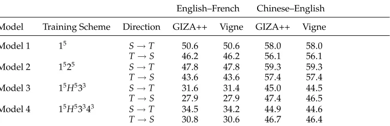
Table 6 shows the alignment error rate percentages for various IBM models in GIZA++ and Vigne. To make the results comparable, we ensured that Vigne shared

Table 6

Comparison of AER scores for various IBM models in GIZA++ and Vigne. These models are trained only on development and test sets. The pruning setting for Vigne isβ=0 andb=1. All differences are not statistically significant.

English–French Chinese–English

Model Training Scheme Direction GIZA++ Vigne GIZA++ Vigne

the same parameters with GIZA++.6 Table 6 also gives the training schemes used for GIZA++. For example, the training scheme for Model 4 is 15H53343. This notation indicates that five iterations of Model 1, five iterations of HMM, three iterations of Model 3, and three iterations of Model 4 are performed. As the two systems use the same model parameters, the amount of training data will have no effect on the comparison. Therefore, we trained the IBM Models only on the development and test sets. As a re-sult, the AER scores in Table 6 look quite high.

In GIZA++, there exist simple polynomial algorithms to find the Viterbi alignments for Models 1 and 2. We observe that the greedy search algorithm (β=0 andb=1) used by Vigne can also find the optimal alignments. Note that the two systems achieve identical AER scores because there are no search errors.

For Models 3 and 4, maximization over all alignments cannot be efficiently carried out as the corresponding search problem is NP-complete. To alleviate the problem, GIZA++ resorts to a greedy search algorithm. The basic idea is to compute a Viterbi alignment of a simple model such as Model 2 or HMM. This alignment (an intermediate node in the search space) is then iteratively improved with respect to the alignment probability of the refined model by moving or swapping links. In contrast, our search algorithm starts from an empty alignment and has only one operation: adding a link. In addition, we treat the fertility probability of an empty cept in a different way (see Equation B.7). Interestingly, Vigne achieves slightly better results than GIZA++ for both models. All differences are not statistically significant.

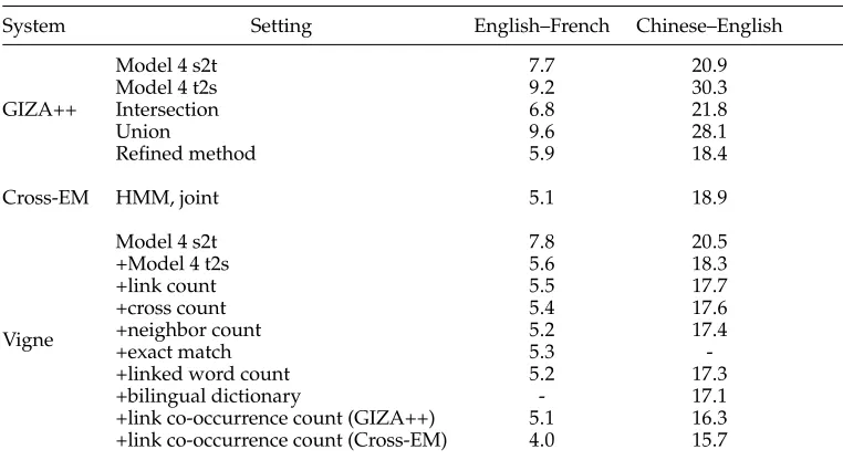
4.1.2 Comparison to Generative Models Using Asymmetric Features. Table 7 compares the AER scores achieved by GIZA++, Cross-EM (Liang, Taskar, and Klein 2006), and Vigne. On both tasks, we lowercased all English words in the training, development, and test sets as a preprocessing step. For GIZA++, we used the default training scheme of 15H53545. We used the three symmetrization heuristics proposed by Och and Ney (2003): intersection, union, and refined method. For Cross-EM, we also used the default configuration and jointly trained Model 1 and HMM for five iterations. For Vigne, we used a greedy search strategy by settingβ=0 andb=1. Note that both GIZA++ and Cross-EM are unsupervised alignment methods.

On the English–French task, the refined combination of Model 4 alignments pro-duced by GIZA++ in both translation directions yields an AER of 5.9%. Cross-EM outperforms GIZA++ significantly by achieving 5.1%. For Vigne, we use Model 4 as the primary feature. The linear combination of Model 4 in both directions achieves a lower AER than either one separately. The link count feature controls the number of links in the resulting alignments and leads to an absolute improvement of 0.1%. With the addition of cross count and neighbor count features, the AER score drops to 5.4%. We attribute this to the fact that the two features are capable of capturing the locality and monotonicity properties of natural languages, especially for closely related language pairs such as English–French. After adding the linked word count feature, our model achieves an AER of 5.2%. Finally, Vigne achieves an AER of 4.0% by combining predictions from refined Model 4 and jointly trained HMM.

On the Chinese–English task, one-to-many and many-to-one relationships occur more frequently in the reference alignments than the English–French task. As Cross-EM

Table 7

Comparison of GIZA++, Cross-EM, and Vigne on both tasks. Note that Vigne yields only one-to-one alignments if both “Model 4 s2t” and “Model 4 t2s” features are used. The pruning setting for Vigne isβ=0 andb=1. While the final results of our system are better than the best baseline generative models significantly at p<0.01, adding a single feature will not always produce a significant improvement, especially for English–French.

System Setting English–French Chinese–English

Model 4 s2t 7.7 20.9

Model 4 t2s 9.2 30.3

GIZA++ Intersection 6.8 21.8

Union 9.6 28.1

Refined method 5.9 18.4

Cross-EM HMM, joint 5.1 18.9

Model 4 s2t 7.8 20.5

+Model 4 t2s 5.6 18.3

+link count 5.5 17.7

+cross count 5.4 17.6

+neighbor count 5.2 17.4 Vigne

+exact match 5.3

-+linked word count 5.2 17.3 +bilingual dictionary - 17.1 +link co-occurrence count (GIZA++) 5.1 16.3 +link co-occurrence count (Cross-EM) 4.0 15.7

is prone to produce one-to-one alignments by encouraging agreement, symmetrizing Model 4 by refined method yields better results than Cross-EM. We observe that the ad-vantages of adding features such as link count, cross count, neighbor count, and linked word count to our linear model continue to hold, resulting in a much lower AER than both GIZA++ and Cross-EM. The addition of the bilingual dictionary is beneficial and yields an AER of 17.1%. Further improvements were obtained by including predictions from GIZA++ and Cross-EM.

As the IBM models do not allow a source word to be aligned with more than one target word, the activation of the IBM models in both directions always yields one-to-one alignments and thus has a loss in recall. To alleviate this problem, we use a heuristic postprocessing step to produce many-to-one or one-to-many alignments. First, we collect links that have higher translation probabilities than corresponding null links in both directions. Then, these candidate links are sorted according to their translation probabilities. Finally, they are added to the alignments under structural constraints similar to those of Och and Ney (2003).

On the English–French task, this symmetrization method achieves relatively small but very consistent improvements ranging from 0.1% to 0.2%. On the Chinese–English task, the improvements are more significant, ranging from 0.1% to 0.8%. This differ-ence also results from the fact that the referdiffer-ence alignments of the Chinese–English task contain more one-to-many and many-to-one relationships than the English–French task. After symmetrization, the final AER scores for the two tasks are 3.8% and 15.1%, respectively.

Table 8

Resulting feature weights of minimum error rate training on the Chinese–English task (M4ST: Model 4 s2t; M4TS: Model 4 t2s; LC: link count; CC: cross count; NC: neighbor count; LWC: linked word count; BD: bilingual dictionary; LCCG: link co-occurrence count (GIZA++); LCCC: link co-occurrence count (Cross-EM)).

M4ST M4TS LC CC NC LWC BD LCCG LCCC

M4ST 1.00 - - -

-+M4TS 0.63 0.37 - - - -+LC 0.18 0.07 −0.75 - - - -+CC 0.19 0.07 −0.56 −0.18 - - - - -+NC 0.12 0.06 −0.55 −0.08 0.17 - - - -+LWC 0.14 0.08 −0.22 −0.08 0.25 −0.26 - - -+BD 0.07 0.02 −0.35 −0.05 0.16 0.01 0.34 - -+LCCG 0.03 0.04 −0.13 −0.05 0.20 −0.16 0.28 0.11 -+LCCC 0.02 0.02 0.14 −0.03 0.10 −0.26 0.30 0.04 0.09

of other features. The weights of the cross count feature are consistently negative, suggesting that crossing links are always discouraged for Chinese–English. Also, the positive weights of the neighbor count feature indicate that monotonic alignments are encouraged. When the bilingual dictionary was included, the weights of Model 4 features in both directions dramatically decreased.

4.1.4 Results of the Symmetric Alignment Model.As we mentioned before, the linear model can model many-to-many alignments directly without any postprocessing symmetriza-tion heuristics.

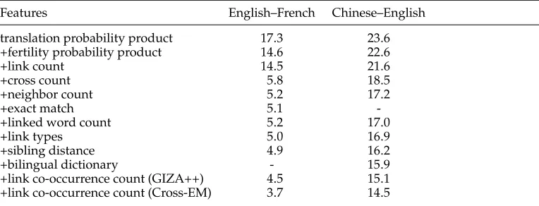
Table 9 demonstrates the results of the symmetric alignment model on both tasks. As the activation of translation and fertility probability products allows for arbitrary relationships, the addition of the link count feature excludes most loosely related links

Table 9

AER scores achieved by the symmetric alignment model on both tasks. The pruning setting for Vigne isβ=0 andb=1. Although the final model obviously outperforms the initial model significantly at p<0.01, adding a single feature will not always result in a significant improvement, especially for English–French.

Features English–French Chinese–English

translation probability product 17.3 23.6 +fertility probability product 14.6 22.6

+link count 14.5 21.6

+cross count 5.8 18.5

+neighbor count 5.2 17.2

+exact match 5.1

-+linked word count 5.2 17.0

+link types 5.0 16.9

and results in more significant improvements than for asymmetric IBM models. One interesting finding is that the cross count feature is very useful, leading to dramatic absolute reduction of 8.7% on the English–French task and 3.1% on the Chinese–English task, respectively. We find that the advantages of adding neighbor count and linked word count still hold. By further including predictions from GIZA++ and Cross-EM, our linear model achieves the best result: 3.7% on the English–French task and 14.5% on the Chinese–English task.

We find that the symmetric linear model outperforms the asymmetric one, espe-cially on the Chinese–English task. This suggests that although the asymmetric model can produce symmetric alignments via symmetrization heuristics, the “genuine” sym-metric model produces many-to-many alignment in a more natural way.

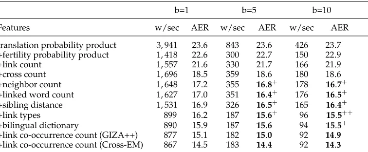
4.1.5 Effect of Beam Search.Table 10 shows the effect of varying beam widths. The aligning speed (words per second) decreases almost linearly with the increase of beam widthb. For simple alignment models such as using only the translation probability product feature, enlarging the beam size fails to bring improvements due to modeling errors. When more features are added, the model becomes more expressive. Therefore, our system benefits from larger beam size consistently, although some benefits are not significant statistically. When we setb=10, the final AER scores for the English–French and Chinese–English tasks are 3.6% and 14.3%, respectively.

4.1.6 Effect of Training Corpus Size. One disadvantage of our approach is that we need a hand-aligned training corpus for training feature weights. However, compared with building a treebank, manual alignment is far less expensive because one annotator only needs to answer yes–no questions: Should this pair of words be aligned or not? If well trained, even a non-linguist who is familiar with both source and target languages could

Table 10

Comparison of aligning speed (words per second) and AER score with varying beam widths for the Chinese–English task. We fixβ=0.01.Boldnumbers refer to the results that are better than the baseline but not significantly so. We use “+” to denote the results that outperform the best baseline (b=1) and are statistically significant at p<0.05. Similarly, we use “++” to denote significantly better than baseline at p<0.01.

b=1 b=5 b=10

Features w/sec AER w/sec AER w/sec AER

translation probability product 3, 941 23.6 843 23.6 426 23.7 +fertility probability product 1, 418 22.6 300 22.7 150 22.9 +link count 1, 557 21.6 330 21.7 166 21.9 +cross count 1, 696 18.5 359 18.6 180 18.6 +neighbor count 1, 648 17.2 355 16.8+ 178 16.7+ +linked word count 1, 627 17.0 351 16.4+ 176 16.5+ +sibling distance 1, 531 16.9 326 16.5+ _{165 16.4}+

+link types 899 16.2 187 15.6+ _{96 15.5}++

produce high-quality alignments. We estimate that aligning a sentence pair usually takes only two minutes on average.

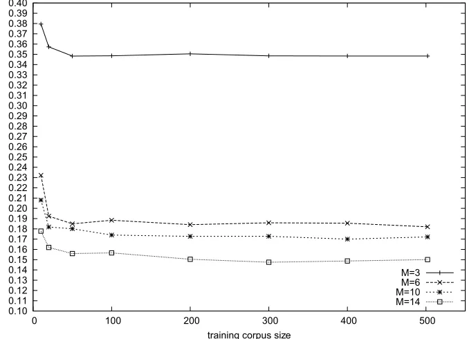
An interesting question is: How many training examples are needed to train a good discriminative model? Figure 4 shows the learning curves with different numbers of features on the Chinese–English task. We choose four feature groups with varying numbers of features: 3, 6, 10, and 14. There are eight fractions of the training corpus: 10, 20, 50, 100, 200, 300, 400, and 502. Generally, the more features a model uses, the more training examples are needed to train feature weights. Surprisingly, even when we use 14 features, 50 sentences seem to be good enough for minimum error rate training. This finding suggests that our approach could work well even with a quite small training corpus.

4.1.7 Summary of Results. Table 11 summarizes the results on all three shared tasks. Vigne used the same configuration for all tasks. We used the symmetric linear model and activated all features. The pruning setting is β=0.01 and b=10. Our system outperforms the systems participating in all the three shared tasks significantly.

Note that for the English–French task we used the small development set of 37 sentences to optimize feature weights, and ran our system on the original test set of 447 sentences. For the Romanian–English language pair, we follow Fraser and Marcu (2006) in reducing the vocabulary by stemming Romanian and English words down to their first four characters. For the other language pairs, English–Inuktitut and English– Hindi, the symmetric linear model maintains its superiority over the asymmetric linear model and yields better results than the other participants.

Figure 4

Table 11

Comparison with the systems participating in the three shared tasks. “non-null” denotes that the reference alignments have no null links, “null” denotes that the reference alignments have null links, “limited” denotes only limited resources can be used, and “unlimited” denotes that there are no restrictions on resources used.

Shared Task Task Participants Vigne

Romanian–English, non-null, limited 28.9–52.7 23.5 Romanian–English, null, limited 37.4–59.8 26.9 HLT-NAACL 2003

English–French, non-null, limited 8.5–29.4 4.0 English–French, null, limited 18.5–51.7 4.6

English–Inuktitut, limited 9.5–71.3 8.9 ACL 2005 Romanian–English, limited 26.6–44.5 24.7 English–Hindi, limited 51.4 44.8

HTRDP 2005 Chinese–English, unlimited 23.5–49.2 14.3

4.1.8 Comparison to Other Work.In the word alignment literature, the Canadian Hansard bilingual corpus is the most widely used data set. Table 12 lists alignment error rates achieved by previous work and our system. Note that direct comparisons are problem-atic due to the different configurations of training data, development data, and test data. Our result matches the state-of-the-art performance on the Hansard data (Lacoste-Julien et al. 2006; Moore, Yih, and Bode 2006).

4.2 Evaluation of Translation Quality

In this section, we report on experiments with Chinese-to-English translation. To inves-tigate the effect of our discriminative model on translation performance, we used three translation systems:

1. Moses(Koehn and Hoang 2007), a state-of-the-art phrase-based SMT system;

2. Hiero(Chiang 2007), a state-of-the-art hierarchical phrase-based system; 3. Lynx(Liu, Liu, and Lin 2006), a linguistically syntax-based system that

makes use of tree-to-string rules.

Table 12

Comparison of some word alignment systems on the Canadian Hansard data.

System Training Test AER

For all three systems we trained the translation models on the FBIS corpus (7.2M+9.2M words). For the language model, we used the SRI Language Modeling Toolkit (Stolcke 2002) to train a trigram model with modified Kneser-Ney smoothing on the Xinhua portion of the Gigaword corpus. We used the 2002 NIST MT evaluation test set as the development set for training feature weights of translation systems, the 2005 test set as the devtest set for choosing optimal values ofαfor different translation systems, and the 2008 test set as the final test set. Our evaluation metric is case-sensitive BLEU-4, as defined by NIST, that is, using the shortest (as opposed to closest) reference length for brevity penalty.

We annotated the first 200 sentences of the FBIS corpus using the Blinker guidelines (Melamed 1998). All links are sure ones. These hand-aligned sentences served as the training corpus for Vigne. To train the feature weights in our discriminative model using minimum-error-rate training (Och 2003), we adopt balanced F-measure (Fraser and Marcu 2007b) as the optimization criterion.

The pipeline begins by running GIZA++ and Cross-EM on the FBIS corpus. We used seven generative alignment methods based on IBM Model 4 and HMM as baseline systems: (1) C→E, (2) E→C, (3) intersection, (4) union, (5) refined method (Och and Ney 2003), (6) grow-diag-final (Koehn, Och, and Marcu 2003), and (7) Cross-EM (Liang, Taskar, and Klein 2006). Instead of exploring the entire search space, our linear model only searches within the union of baseline predictions, which enables our system to align large bilingual corpus at a very fast speed of 3, 000 words per second. In other words, our system is able to annotate the FBIS corpus in about 1.5 hours. Then, we train the feature weights of the linear model on the training corpus with respect to F-measure under different settings ofα. After that, our system runs on the FBIS corpus to produce word alignments using the optimized weights. Finally, the three SMT systems train their models on the word-aligned FBIS corpus.

Can our approach achieve higher F-measure scores than generative methods with different values ofα(the weighting factor in F-measure)? Table 13 shows the results of all the systems on the development set. To estimate the loss from restricting the search

Table 13

Maximization of F-measure with different settings ofα(the weighting factor in the balanced F-measure). We use IBM Model 4 and HMM as baseline systems. Our system restricts the search space by exploring only the union of baseline predictions. We compute the “oracle” alignments by intersecting the union with reference alignments. We use “+” to denote the result that outperforms the best baseline result with statistical significance at p<0.05. Similarly, we use “++” to denote significantly better than baseline at p<0.01.

α=0.1 α=0.3 α=0.5 α=0.7 α=0.9

IBM Model 4 C→E 82.6 81.3 80.1 79.0 77.8 IBM Model 4 E→C 68.2 70.5 73.0 75.7 78.5 IBM Model 4 intersection 63.6 68.9 75.2 82.8 92.1 IBM Model 4 union 86.6 82.0 77.9 74.2 70.8 IBM Model 4 refined method 75.4 78.5 81.8 85.4 89.4 IBM Model 4 grow-diag-final 82.4 82.1 81.7 81.4 81.1 Cross-EM HMM 70.4 73.7 77.3 81.2 85.5

oracle 91.9 93.6 95.3 97.1 99.0