Abstract- Radial Distribution Systems (RDS) connect a large
number of renewable generators that are inherently uncertain. From being unidirectional power flow systems, RDS now enable bi-directional power flow. Depending upon availability of power from renewables, they receive or feed power to the connected transmission system. RDS optimal power flow (OPF), is an important tool in this new era for utilities, to minimize losses and operate efficiently.
With large scale integration of wind generators to distribution systems, they must be appropriately represented using probabilistic models capturing their intermittent nature in these OPF algorithms. This paper proposes characterizing the solution of a Probabilistic Optimal Power Flow (P-OPF) for RDS using the Cumulant Method. This method makes it possible to linearly relate the probabilistic parameters of renewables at the optimal solution point to the state of the RDS. To assess the accuracy of the proposed P-OPF Cumulant Method, wind generators and system probabilistic data are incorporated in a 33-bus and 129-bus test system. The results are compared with those of Monte Carlo simulations (MCS). It is shown that the proposed method possesses high degree of accuracy, is significantly faster and more practical than an MCS approach.
NOMENCLATURE PD, QD
SD T ST PT QT PW PL TPL V NB SB QS U Y
Vector of bus-wise real and reactive power loads
Apparent power loads Tap Setting
Total Apparent Power Total Real Power Total Reactive Power
Vector of real power output of WGs System Real Power Loss
System Total Real Power Loss Vector of bus voltages magnitudes Number of buses in the system
The difference between generation and load Reactive power injected into the ith bus
Decision vector in the optimization problem
Dependent vector in the optimization problem
Independent random input variables Output variable created by linear combination of “n” independent random
Financial Support: This work was supported in part by the NSERC Discovery and WesNet grants to Bala Venkatesh
M. Dadkhah and B. Venkatesh are with Ryerson University, Toronto, Canada (e-mails: maryam.dadkhah@ryerson.ca and bala@ryerson.ca).
s Φ(s) Ψ(s) K,m
K,m
OPF H KsB,n
P-OPF PDF RDS WG MCS CM LBIPM KKT
input variables Complex frequency
Moment Generating Function Cumulant Generating Function
Vector containing the mth order cumulants of the system unknown variables
Vector containing the mth order cumulants of the system known variables
Optimal Power Flow Hessian of the Lagrangian
Vector of -order Cumulants for the random bus power injections
Probabilistic Optimal Power Flow Probability Density Function Radial Distribution Systems Wind Generator
Monte Carlo Simulations Cumulant Method
Logarithmic-Barrier Interior Point Method Karush–Kuhn–Tucker Conditions
I. INTRODUCTION
O
PF (optimal power flow) is a versatile tool used for electric transmission systems for a variety of purposes. The most common amongst them are: (a) real power OPF where real power output of generators are scheduled such that the total cost of generation is minimized [1], and, (b) reactive power OPF where generators voltages, reactive power compensation and settings of transformers taps are set to route reactive power optimally such that real power transmission losses are the least and all the voltages are within prescribed limits [2]. OPF has not been easily extended to distribution systems as their system Jacobian is ill-conditioned owing to higher R/X ratio of their lines [15]. In the recent past, numerous Jacobian based OPF methods have been researched and published [3]. Today, with a rush to integrate wind generators to electric power systems, largely to distributions systems, distribution systems OPF must account for wind generators as well.In essence, an OPF for distribution systems must contend with the challenge that it must account for wind generators that are uncertain in their output and their near term forecasts can be best represented by a normal distribution with mean and variance values [16]. Further to understand the effect of probabilistic nature of loads and availability of wind on the OPF solution, such as the optimal values of transformer taps and capacitor settings, it is necessary to propose an efficient probabilistic OPF method that includes the load and generator probabilistic models.
Probabilistic - Optimal Power Flow for Radial
Distribution Systems with Wind Generators
The ultimate goal is to determine the probability density function of typical variables such as voltage and power flow that form a part of OPF solution.
Uncertainties of the power systems components have been addressed with many researchers by adapting probabilistic techniques in the Power Flow solution in transmission systems since 1960s [4]. Later, the probabilistic methods were applied to the optimal dispatch [5] and for the first time the term P-OPF was used in [6]. However, in contrast to the transmission system case, distribution systems have not been studied to the same extent. In [7] the authors proposed a probabilistic optimal capacitor planning method using Cumulant technique to find the probabilistic information of the size of newly installed capacitor banks in the distribution systems with high penetration of wind generations.
This paper uses the idea given in [7] to propose and construct a distribution system OPF using a set of 3N equations such that the Jacobian is robust [8]. The objective of the OPF is to minimize losses in the distribution system by optimally scheduling all the reactive power sources and ensuring that voltages are within the prescribed limits. Then, it proposes to use Cumulant Method (CM) to directly relate probabilistic values of the loads and output power of wind generators to the optimal settings of the distribution system [9]. This approach has been reported for uncertainty without specific application to wind generators and in transmission system by A. Schellenberg et. al. [10].
This paper is outlined as follows. In sections 2 and 3, the model of the radial distribution system for OPF solution is presented and the Cumulant method is described respectively. Section 4 presents the numerical results of the method as tested on the 33-bus IEEE test system with three wind generators and a 129-bus test system with nine wind generators. Section 5 concludes the paper.
II. SYSTEM MODEL AND PROBABILISTIC OPF A. Problem Formulation
[image:2.595.50.274.583.673.2]This subsection uses the radial distribution system (RDS) model from [8]. Fig. 1 shows a single-line representation of a tree-like distribution systems structure.
Fig. 1 A tree-like distribution system with wind generator
Consider the ith bus in Fig. 1. It has a wind turbine connected to it that injects only real power equal to PWi. Its
bus load is represented by SDi = PDi + j.QDi. The total
power injected into this bus is SBi = SDi - PWi. It is the
difference between generation and load at that bus. Consider the lth line/transformer between buses i-1 and i. The tap
setting of this transformer/line is represented by Tl and it has
an impedance of Zl = Rl + jXl. The total apparent power reaching the downstream end of this line equals STl . The
real power loss on this line equals:
2 i 2 V ST R
PLl l l (1)
The total real power loss in all feeders of the system equals:
nl 1 2 i 2 V ST R TPLl l l (2)
where Vi is the bus voltage magnitude, nb is the number of buses in the system and nl is the number of lines/transformers.
In Fig. 1, the complex power balance at the ith can be expressed as: i i k3 3, k k1 1, k k , k 2 k 2 i
i SD Z.ST .V ST PW j QS
ST
l l l ll (3)
Where QSi is the reactive power injected into the ith bus.
Equation (3) is a complex equation and yields a set of 2(NB-1) equations. Writing the voltage drop equation across line l gives: 0 ST . Z T V . 2 1 .X QT .R PT . 2.V
V 2 2 2
2 1 i 2 i 4
i
l l l l l l
l (4)
Equations (3) and (4) provide 3(NB-1) equations that completely model a RDS.
B. OPF for Radial Distribution System
The objective of Radial Distribution System OPF is to minimize the total real power loss. By referring to the set of equations (2) – (4), one may construct an optimal power flow formulation for a radial distribution system as below:
Objective Function:
Minimize:
nl 1 2 i 2 V ST R TPL
l l l (5)
Constraints: i i k3 3, k k1 1, k k , k 2 k 2 i
i SD Z.ST .V ST PW j QS
ST
l l l ll (6)
0 ST . Z T V . 2 1 .X QT .R PT . 2.V
V 2 2 2
2 1 i 2 i 4
i
l l l l l l
l (7)
UMIN < U < UMAX (8)
VMIN < V < VMAX (9)
where the decision vector is U = [QS , T] and dependent vector is Y = [V, P, Q]. Equations (6)-(7) are equality constraints which correspond to the complex power balance equation and the voltage drop equation across line l, respectively. Equations (8) and (9) limit the control and dependent vectors. The optimization problem described by (5)-(9) is solved by using the Logarithmic-Barrier Interior Point Method (LBIPM) [11].
Tl
i-1 i
PWi
SDi
SBi
STl
Rl + j. Xl
C. Optimal Solution
The formulation (5)-(9) is solved using the Lower Bound Interior Point Method [11]. This yields the optimal solution of decision and dependent vectors U and Y. In addition, the Hessian of the Lagrangian formed from the optimization formulation (5)-(9) is evaluated H (U, Y, λ). It provides a linear relation between incremental changes of dependent vector in terms of the decision vector.
III. CUMULANT TECHNIQUE AND P-OPF
In probability theory, Cumulants and moments are two sets of quantities of a random variable which are mathematically equivalent. However, in some cases preference is to use Cumulants due to their simplicity over using moments [12]. In this section some properties of Cumulants used to adapt the Cumulant Technique to the radial distribution system P-OPF are presented.
Consider a linear combination of ‘n’ independent random input variables α used to create a new random output variable β as follows [10]:
= c1 . 1 + c2 . 2 + c3 . 3 + … + cn . n (10)
where ci is the ith coefficient in the linear combination. The above expansion can be written in terms of the moment generation function of random variable , i.e., (s) , as
(s)
Φ E
e
s E
e
sc11c22...cnn
(11)where s is the Laplace operator. Assuming that α1, α2, α3,
…, αn are independent, the above relationship can be written
as
(s) = E[es] E
e
sc11
Ee
sc22
Ee
scnn
=1(sc1).2(sc2)….n(scn) (12)
The Cumulant generating functionx(s) can be written in
terms of the moment generating function x as [12]
Φ s
. ln (s)Ψ (13)
By taking the natural logarithm at both sides of the (12) and using (13), (12) is written in the terms of cumulant generating function as below:
. ) (sc Ψ ... ) (sc Ψ ) (sc Ψ (s)
Ψβ α1 1 α2 2 αn n (14)
To obtain the different orders of cumulants, we can set
0
s to compute the different order derivatives of the cumulant generating function. A general equation for the mth
order cumulant of Ψ is
0 c Ψ
0 ... c Ψ
0Ψ . c (0)
Ψ(m) 1m αm1 m2 αm2 nm αmn (15)
0 ... c K
0. K. c K . c
K,m 1m 1,m m2 2,m nm n,m (16)
where Kβ,m is a vector containing the mth order cumulants
of the system unknown variables and Kα,m is a vector
containing the mth order cumulants of the random bus
generation and loading.
A. Adaptation to P-OPF
By applying Newton method to the Lagrangian function L (U, Y, λ) for (5)-(9), the following system is obtained:
0 λ Y U λ) Y, H(U, λ) Y,
L(U,
(17)
where L(U,Y,) and H(U,Y, λ) are the gradient and the Hessian of the Lagrangian respectively. Rearranging (16) and replacing L(U,Y,)with a vector of change in the bus power injections for uncertain wind power, ∆SB, the vector of changes can be linearly mapped with ∆SB by using the inverse of the Hessian:
SB λ) Y, L(U, λ)
Y, H(U, λ
Y U
Y U,
1 (18)
By replacing ∆SB with a vector containing the nth order
cumulants of loads and generation, the Cumulants of system variables, ∆SB can obtain using the inverse of the Hessian as follow:
n SB, (n) 1 n
), Y,
(U, K
0 H
K (19)
where K(U,Y,λ),n is a vector of nth -order cumulants for the
optimal settings of the distribution system and KSB,n is a
vector of nth -order Cumulants for the random bus power
injections. Consequently, the Hessian contains the constant multipliers. Once the cumulants of the random variables of the OPF solution are computed from the input random variables, PDFs are recreated by using Gram-Charlier/Edgeworth Expansion theory [13].
IV. NUMERICAL RESULTS
This section provides the results based on applying the Cumulant method to the 33-bus and 129-bus test systems. In both systems, the loads and the power output of wind generators are considered Gaussian random variables with the mean values set to the nominal bus loading and mean capacity of wind generators respectively. The standard deviation is such that the 99% confidence interval is equal to ±%15 of the nominal loading value. In order to show the efficiency and accuracy of the Cumulant method, the results have been compared with MCS with 5000 samples.
A. 33-Bus Test System Case Study
The method is firstly applied to the 33-bus, 32-branch IEEE test system described in [14]. The system, however, is modified to accommodate the probabilistic data of the loads and wind generators. The modified system and loads data can be found in the Appendix. Three wind turbines are connected to buses 3, 17 and 32 with a mean capacity equal to 500 kW each. The results of both mean and standard deviation values obtained by comparing with those of 5000 sample points MCS, are discussed as follows.
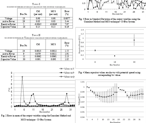
occurs at bus 18 and is as low as 0.1901%. These results show a small difference between two methods in systems variables mean values which can be seen more clearly in Fig. 2.
2) Variance Value: The maximum percentage errors for the system variables variance values are presented in Table II. These values for the voltage, active power, reactive power and capacitor value variance are equal to 1.55%, 1.91%, 2.13% and 1.85% which occur at buses 24, 9, 11 and 30 respectively. These small error values for the variance of the systems variables are shown in Fig. 3.
In summary, the percentage errors of the mean and variance values for the system variables are well below 8% which implies a close match between two methods. Also, it is worth noting that largest errors (8%) occur for reactive power and voltage magnitude variables due to inherent nonlinearity. This nonlinearity for voltage and reactive power usually happens in the buses with capacitor banks connected to them.
TABLE I
MAXIMUM ERROR OF MEAN VALUES OF THE SYSTEM VARIABLES
Bus No.
CM (per unit)
MCS (per unit)
Error (%)
Voltage 18 0.98 0.98 0.0077
Active Power 29 0.03 0.03 3.44 Reactive Power 5 -0.0045 -0.0049 7.97 Capacitor Value 18 0.15 0.15 0.19
TABLE II
MAXIMUM ERROR OF VARIANCE VALUES OF THE SYSTEM VARIABLES
Bus No. CM MCS
Error (%)
Voltage 24 0.0013 0.0012 1.55
Active Power 9 0.079 0.0811 1.91 Reactive Power 11 0.0062 0.0061 2.13 Capacitor Value 30 0.091 0.093 1.85
0 1 2 3 4 5 6 7 8 9
1 6 11 16 21 26 31
[%
]
Bus number
[image:4.595.321.562.242.378.2]%Error in V %Error in P %Error in Q
Fig. 2 Error in mean of the output variables using the Cumulant Method and MCS technique - 33-Bus System
The analysis using Cumulant method is captured in graphs of Fig. 4 and 5 wherein mean capacitor and bus voltage magnitude values are shown with potential spread using corresponding 3σ values. This analysis and graphing can be rapidly completed using the proposed method.
Table III presents the time comparison between Cumulant method and Monte Carlo Simulation technique. It is evident that to identify this spread in values of capacitor settings and voltages at buses, though being important information, is difficult to obtain using the conventional Monte Carlo Simulation technique due to long solution time. However, using the proposed cumulant method, using a few additional steps such as computation of the Hessian of the Lagrangian, yields the variance values of the optimized control (capacitor) and dependent (voltage) variables.
Fig. 3 Error in Standard Deviation of the output variables using the Cumulant Method and MCS technique– 33-Bus System
Fig. 4 Mean capacitor values are shown with potential spread using corresponding 3σ values.
Fig. 5 Mean bus voltage magnitude values are shown with potential spread using corresponding 3σ values.
0 0.5 1 1.5 2 2.5
1 6 11 16 21 26 31
[%
]
Bus number
%Error in V %Error in P %Error in Q
0 0.2 0.4 0.6 0.8 1 1.2 1.4
8 18 30
R
ea
ct
iv
e P
o
we
r
[P
.U
.]
Bus Number
0.94 0.95 0.96 0.97 0.98 0.99 1 1.01
1 4 7 10 13 16 19 22 25 28 31
Vo
lta
ge
[P
.U
.]
[image:4.595.43.554.326.754.2]This is an important benefit for the RDS operator as s/he would like to how far the capacitor values and voltage solutions might travel from the mean forecasted and anticipate/plan to avoid violations.
TABLE III
TIME COMPARISON BETWEEN CUMULANT METHOD AND MONTE CARLO
SIMULATION TECHNIQUE
Execution
Time (seconds) CM MCS
System #1 4.44 seconds seconds. 2888.05
B. The 129-Bus Test System Case Study
To show the accuracy and efficiency of the Cumulant method, it also has been tested on a large system of 129-bus with nine wind generators each having a mean capacity equal to 500 kW. The results have been compared with 5000 sample points of MCS.
Table IV shows the mean absolute percentage error of mean and standard deviation of the problem variables.
TABLE IV
MEAN ABSOLUTE PERCENTAGE ERROR OF MEAN AND STANDARD
DEVIATION OF THE PROBLEM VARIABLES
Variable
Mean Standard Deviation
Voltage 0.0025 1.4285
Real Power 0.2206 0.8180
Reactive Power 0.4580 1.2150
Capacitor Size 0.0589 1.2537
TABLE V
TIME COMPARISON BETWEEN CUMULANT METHOD AND MONTE CARLO
SIMULATION TECHNIQUE
Execution Time (seconds)
CM MCS System #2 12.79 seconds 6504.87
seconds.
The method works well for small and reasonably sized systems.
V. CONCLUSION
This paper describes the Cumulant method for probabilistic optimization of radial distribution systems. Random variables used in distribution system are the output of wind generators and bus loads. Both are modeled using Gaussian distribution function. While a Logarithmic Barrier Interior Point Method (LBIPM) based solver is used to solve the probabilistic nonlinear optimization problem, the cumulants of the system variables are easily computed using the inverse of the Hessian of the Lagrangian function.
The method was implemented and tested on a 33-bus and 129-bus IEEE test system. In order to illustrate efficiency and accuracy of the cumulant method, the resultant data using cumulant method are benchmarked with those obtained from Monte Carlo Simulation Technique with 5000 samples. The errors were found well below 8%. An execution time comparison demonstrates superiority of the Cumulant method. Less computational burden and complexity makes the proposed method very practical and advantageous.
This method can be advantageously used by RDS operators to know possible swings in optimal capacitor settings and voltage solution giving them additional insight into operation of the system and anticipate potential operational challenges.
APPENDIX
Table VI presents the mean values used for the load demands, and Table VII presents the feeder data.
TABLE VI
33BUS RDS-MEAN VALUE OF THE LOADS
Bus Number
Mean
Real Power (kW) Reactive Power (kW)
1 0 0.0
2 0.1 0.06
3 -0.5 0.0
4 0.12 0.08
5 0.06 0.03
6 0.2 0.1
7 0.2 0.1
8 0.2 0.1
9 0.06 0.02
10 0.06 0.02
11 0.045 0.03
12 0.06 0.035
13 0.06 0.035
14 0.06 0.04
15 0.06 0.01
16 0.09 0.04
17 -0.5 0.0
18 0.09 0.04
19 0.09 0.04
20 0.09 0.04
21 0.09 0.04
22 0.09 0.04
23 0.09 0.05
24 0.42 0.2
25 0.42 0.2
26 0.06 0.025
27 0.06 0.025
28 0.06 0.02
29 0.12 0.07
30 0.2 0.6
31 0.15 0.07
32 -0.5 0.1
TABLE VII
33BUS RDS-LINE DATA
From Bus
To
Bus R (Ω) X (Ω)
Rating (MVA)
System Voltage (kV)
1 2 0.0922 0.047 100 12.66
2 3 0.493 0.2511 100 12.66
3 4 0.3662 0.1864 100 12.66
4 5 0.3811 0.1941 100 12.66
5 6 0.819 0.707 100 12.66
6 7 0.1872 0.6188 100 12.66
7 8 1.7114 1.2351 100 12.66
8 9 1.03 0.74 100 12.66 9 10 1.044 0.74 100 12.66
10 11 0.1966 0.065 100 12.66
11 12 0.3744 0.1238 100 12.66
12 13 1.468 1.155 100 12.66
13 14 0.5416 0.7129 100 12.66
14 15 0.591 0.526 100 12.66
15 16 0.7463 0.545 100 12.66
16 17 1.289 1.721 100 12.66 17 18 0.732 0.574 100 12.66
18 19 0.164 0.1565 100 12.66
19 20 1.5042 1.3554 100 12.66
20 21 0.4095 0.4784 100 12.66
21 22 0.7089 0.9373 100 12.66
22 23 0.4512 0.3083 100 12.66
23 24 0.898 0.7091 100 12.66
24 25 0.896 0.7011 100 12.66
25 26 0.203 0.1034 100 12.66
26 27 0.2842 0.1447 100 12.66
27 28 1.059 0.9337 100 12.66
28 29 0.8042 0.7006 100 12.66
29 30 0.5075 0.2585 100 12.66
30 31 0.9744 0.963 100 12.66
31 32 0.3105 0.3619 100 12.66
32 33 0.341 0.5302 100 12.66
ACKNOWLEDGMENT
Financial Support: This work was supported in part by the NSERC Discovery and WesNet grants to Bala Venkatesh
REFERENCES
[1] J. A. Momoh, M.E. El-Hawary, R. Adapa, “A Review of Selected Optimal Power Flow Literature to 1993 Part I: Non-Linear and Quadratic Programming Approaches,” IEEE Transactions on Power Systems, vol. 14, No. 1, pp. 96–104, Feb. 1990.
[2] K.R.C. Mamandur, R. D. Chenoweth, “Optimal Control of Reactive Power Flow for Improvements in Voltage Profiles and for Real Power Loss Minimization,” IEEE Transactions on Power Apparatus and Systems, vol. PAS-100, No. 7, pp. 3185-3194, 1981
[3] M. Ponnavsikko, K. S. Prakasa Rao, “Optimal Distribution Systems Planning,” IEEE Transactions on Power Apparatus and Systems, vol. PAS-100, No. 6, pp. 2969 - 2977, June 1981
[4] M. Schilling, A. L. da Silva, and R. Billinton, “Bibliography on power system probabilistic analysis (1962-1988),” IEEE Transactions on Power Systems, vol. 5, no. 1, pp. 1–11, Feb. 1990.
[5] G. Vivian and G. Heydt, “Stochastic energy dispatch,” IEEE Transactions on Power Apparatus and Systems, vol. 100, no. 7, pp. 3221–3227, 1981.
[6] M. El-Hawary and G. Mbamalu, “A comparison of probabilistic perturbation and deterministic based optimal power flow solutions,” IEEE Transactions on Power Systems, vol. 6, no. 3, pp. 1099–1105, Aug 1991.
[7] M. Dadkhah, B. Venkatesh, “Cumulant Based Stochastic Reactive Power Planning Method for Distribution Systems With Wind Generators,” IEEE Transactions on Power Systems, vol. 27, pp. 2351 – 2359, Nov. 2012
[8] A. Dukpa, B. Venkatesh and L. Chang, An Accurate Voltage Solution Method of Radial Distribution System, Canadian Journal for Electrical and Computer Engineering, 34 (1/2): 69 – 74, Win/Spr 2009.
[9] A. Papoulis and S. Pillai, Probability, Random Variables, and Stochastic
Processes, 4th ed. New York: McGraw-Hill, 2002.
[10] A. Schellenberg, W. Rosehart, and J. Aguado, “Cumulant based probabilistic optimal power flow (P-OPF),” in Proceedings of the 2004 International Conference on Probabilistic Methods Applied to Power Systems, Sept 2004, pp. 506–511
[11] G. O. G. Torres and V. Quintana, “An interior-point method for nonlinear optimal power flow using voltage rectangular coordinates,” IEEE Trans. Power Syst., vol. 13, no. 4, pp. 1211–1218, Nov. 1998. [12] A. Schellenberg, W. Rosehart, and J. Aguado, “Introduction to
cumulant-based probabilistic optimal power flow (P-OPF),” IEEE Trans. on Power Systems, vol. 20, no. 2, pp. 1184–1186, May 2005. [13] P. Zhang and S. T. Lee, “Probabilistic load flow computation using
the method of combined cumulants and Gram –Charlier expansion,”IEEE Trans. Power Syst., vol. 19, no. 1, pp. 676–682, Feb. 2004.
[14] M. A. Kashem, V. Ganapathy, G. B. Jasmon, M. I. Buhari. “A Novel Method for Loss Minimization in Distribution Networks.” International Conference on Electric Utility Deregulation and Restructuring and Power Technologies 2000.
[15] S. C. Tripathy, D. Prasad, O. P. Malik and G. S. Hope, Load flow solution for ill conditioned power systems by Newton like method, IEEE Transactions on Power Apparatus and Systems, 101: 3648-657, 1982.