Monte Carlo Pricing Scheme for a
Stochastic-Local Volatility Model
Geoffrey Lee, Yu Tian, and Zili Zhu
Abstract—We have developed a Monte Carlo engine for using a hybrid stochastic-local volatility (SLV) model to price exotic options. Through a case study where AUD/USD FX market data is used, we demonstrate that the implemented SLV model can reproduce market implied volatilities. A PDE pricing engine for the SLV model has been used as the benchmark to examine the performance of the Monte Carlo engine for which two different control variates are implemented to reduce the pricing variance in the raw Monte Carlo results. The numerical results shown in this paper suggest that the best improvement in accuracy is obtained when utilising market-traded exotic options as a control variate to price another exotic option, whereas using the conventional vanilla option as a control variate is not effective for the SLV model.
Index Terms—stochastic local volatility, exotic options
I. INTRODUCTION
C
URRENTLY, a class of volatility models that com-bine the advantages of both the local volatility model and stochastic volatility models have become very popular, particularly in the finance industry [1]–[4]. This class of models, termed stochastic-local volatility models, combine the local volatility model of Dupire [5] with a stochastic volatility model. Different stochastic volatility models such as the Heston model [2], [4] or the SABR model [6] have been used to construct such stochastic volatility models.Our hybrid model presented in this paper consists of a non-linear and non-parametric combination of a pure local volatility model and a pure Heston stochastic volatility model. The impacts of the two models are controlled by a function termed the leverage function, in addition to a parameter termed the mixing fraction.
A brief description of our hybrid SLV model is presented in Section II, where we outline the calibration procedure in addition to the two different pricing methods used. A more detailed description of both the calibration and pricing procedures can be found in [7]. We then present a case study examining the performance of Monte Carlo pricing techniques using market data for the AUD/USD currency pair. In particular, we will focus on improving the pricing accuracy of the Monte Carlo method by utilising a control variate to reduce the sample variance, because in the context of the stochastic-local volatility model, market prices for certain exotic options are available in calibrating the model, and therefore the available market prices can also be used effectively for control-variate techniques.
G. Lee and Z. Zhu are with CSIRO Computational Informatics, Clayton, VIC, Australia, Email:{Geoffrey.Lee,Zili.Zhu}@csiro.au.
Y. Tian is with School of Mathematical Sciences, Monash University, Clayton, VIC, Australia. Email: [email protected]
II. STOCHASTICLOCALVOLATILITYMODEL
Our implementation of the stochastic-local volatility model is assumed to follow Heston-like dynamics. Under the risk neutral measure, the SLV model for two FX rates with the same domestic currency is
dSt= (rd−rf)Stdt+L(St, t)
p
VtStdW (1)
t , S0=s,
dVt=κ(θ−Vt)dt+λ
p
VtdW (2)
t , V0=v,
dWt(1)·dW (2) t =ρdt,
(1) where rd is the domestic interest rate and rf the foreign interest rate in the context of FX market, both of which are assumed to be locally deterministic with term structure. We denote r =rd−rf in the following sections. We also assume that the Heston parameters – the mean-reversion rate
κ, the mean-reversion levelθ, the volatility of volatilityλand correlationρ– all have time-dependent term structures. The functionL(St, t), termed the leverage function, controls the impact of local volatility.
According to the mimicking theorem presented in [8], the marginal distribution of the SLV model described by Equation (1) is identical to the distribution of a local volatility model [5], [9] with the local volatilityσLV(S, t)given by
σLV(x, t)2 = E[L(St, t)2Vt|St=x]
= L(x, t)2E[Vt|St=x] (2) If we calibrate the local volatility model to the market, the mimicking theorem ensures that the hybrid SLV model can match the price from the local volatility model and therefore can reproduce the vanilla market prices. By introducing the transition probability density of the LSV model, p(S, V, t), we can write the leverage function as
L(x, t) = pσLV(x, t)
E[Vt|St=x]
= σLV(x, t)
v u u t
R
R+p(x, V, t)dV
R
R+V p(x, V, t)dV
. (3)
A. Calibration
function. The Fokker-Planck equation for the transition prob-ability density under the SLV model is given by
∂p ∂t =−
∂
∂S[rSp]− ∂
∂V[κ(θ−V)p]+
+1 2
∂2
∂S2[L
2S2V p] + ∂2
∂S∂V[λρLSV p] + 1 2
∂2
∂V2[λ 2V p].
(4) In addition to available vanilla market data as input data, some traded exotic option market prices are also available. We therefore want our model to reproduce traded exotic option market prices as well. To this end, we introduce a parameterη ∈[0,1], termed the mixing fraction, that is used to multiply both the volatility of volatility parameter λ in addition to the correlation parameterρ. The mixing fraction controls the impact of the pure stochastic volatility; when the mixing fraction is 0, the local stochastic model degenerates into a pure local volatility model, while as the mixing fraction increases towards 1, the impact of the stochastic volatility increases. To complete the calibration process, we determine the term-structure of the mixing fraction by using a non-linear optimization routine to minimize the relative error between the SLV model price and the input market prices for vanilla and exotic options. If exotic options are present in the calibration, we can choose to have different optimisation weighting on the exotic options’ prices. However, for the nu-merical results of this paper, we choose to only include errors from pricing the input exotic options for the optimisation.
To summarize, the calibration procedure of the SLV model is implemented as follows:
Calibration:
1) For given market data including implied volatilities, calibrate the parameters in term-structure form for Heston stochastic volatility model.
2) For the same market data, generate local volatility surface data.
3) With calibrated Heston parameters and generated local volatilities, calibrate the term-structure of the mix-ing fraction and the leverage function by solvmix-ing the Fokker-Planck equation to match market implied volatilities as well as traded prices of available exotic options.
Note: the first two steps in the calibration phase are independent and they both feed the third calibration step. We refer to [7] and [10] for more details of the calibration.
B. Pricing Implementation
Once we have calibrated the SLV model, we can store the Heston stochastic parameters and the mixing fraction for pricing other exotic options later. For pricing exotic options with different expiries to any maturity tenors, the calibrated leverage function may be interpolated along the spot direction using cubic spline interpolation, and along the time direction using linear interpolation. After calibration, when pricing any new exotic options, we will re-generate the leverage function.
Currently, we have implemented two different numerical methods for using the SLV model to price exotic options: using the finite difference method for solving the pricing PDEs of the SLV model, and using the Monte Carlo simula-tion method for the stochastic equasimula-tions of the SLV model.
In this paper, we will mainly present our numerical results from the Monte Carlo method, and we will only use the implemented finite difference method as the benchmark.
1) Finite Difference Approach: In order to maintain the positivity of the variance process, we choose to transform the original LSV model of(St, Vt)into a model of log-spot and log-variance, such that our new stochastic variables are expressed as(Xt= log(St/S0), Zt= log(Vt/V0)). We note that we have also scaled our original variables by their initial spot values(S0, V0)in making the log transformation.
From Ito’s lemma, the SLV model for log-spot Xt and log-varianceZtbecomes
dXt= [rd(t)−rf(t)−
1
2L(Xt, t)
2V t]dt
+L(Xt, t)
p
VtdW (1) t ,
dZt= [(κθ−
1 2λ
2)1
Vt
−κ]dt+λ√1 Vt
dWt(2),
dWt(1)·dW (2) t =ρdt.
(5)
Here St=S0·eXt,L(Xt, t) :=L(S0·eXt, t) =L(St, t), andVt=V0·eZt.
It would be more intuitive if we can introduceτ =T−t, then the backward option pricing PDE for a payoff function
u(S, V, τ)under the log-transformed SLV model (5) can be transformed to:
∂u
∂τ = [r(τ)− 1 2L
2V]∂u
∂X + 1 2L
2V ∂ 2u
∂X2+λρL
∂2u ∂X∂Z+
+[(κθ−1 2λ
2)1
V −κ] ∂u ∂Z + 1 2λ 21 V ∂2u
∂Z2−rd(τ)u. (6) We can solve the above PDE (6) by an alternating-direction-implicit (ADI) scheme from [11] as
A=un−1+ ∆τn[G0(un−1, τn−1) +G1(un−1, τn−1)+
+G2(un−1, τn−1)],
B−α∆τnG1(B, τn) =A−α∆τnG1(un−1, τn−1),
C−α∆τnG2(C, τn) =B−α∆τnG2(un−1, τn−1),
un=C, n= 1, . . . , N,
(7) with
G0(u, τ) =λρL
∂2u
∂X∂Z +b0(τ), G1(u, τ) = [(κθ−
1 2λ
2)1
V −κ] ∂u ∂Z + 1 2λ 21 V ∂2u
∂Z2−
−1
2rd(τ)u+b1(τ), G2(u, τ) = [r(τ)−
1 2L
2V]∂u
∂X + 1 2L
2V ∂2u
∂X2−
−1
2rd(τ)u+b2(τ).
(8)
Here bi(τ) are boundary conditions imposed in the mixed derivative, Z- and X-directions. The parameter α controls the weight given to an implicit solution for the differential equation. We use a valueα= 1 which ensures stability of the solution in addition to improving the accuracy of pricing options with a discontinuity in the payoff or in the derivatives of the payoff with respect to the spot.
the domains chosen for both the spot and variance. For boundary mesh points, we use a first-order forward or backward finite difference according to the location of the boundary mesh points. We refer to [7], [11] and [12] for more details.
The implementation of initial and boundary conditions for the option payoff function is critical in using a finite difference method to solve the option pricing PDE. The initial and boundary conditions for some FX exotic op-tion payoffs can be found in [10]. Addiop-tionally, boundary conditions for Heston-like models are extensively discussed in [11]–[17]. For pricing digital options where the initial condition (the payoff function) is discontinuous at the strike, we approximate the payoff using the averaging scheme in [18] to ensure accurate finite difference calculations of the first and second order derivatives along the spot direction. The payoff at the strike is taken to be the mid-point (1/2for cash-payment orK/2for asset-payment).
2) Monte Carlo Method: We evolve the spot and variance stochastic differential equations defining the SLV model using the Euler method for M time steps. We ensure that the variance process remains positive by implementing the full truncation scheme as described in [19]. If the variance process becomes negative, we reset its value to be zero. The evolution equations for the spot and variance thus take the following form:
Sti+1=Sti+ [rd(ti)−rf(ti)]Sti∆t+
+L(Sti, ti)
p
VtiSti∆W
(1) ti ,
Vti+1 =Vti+κ(θ−(Vti)
+)∆t+λp
(Vti)
+[ρ∆W1 ti+
+p1−ρ2∆W(2) ti ], Vti+1 = (Vti+1)
+,
(9) with ∆t = ti+1 −ti, ∆W
(j) ti = W
(j) ti+1 −W
(j) ti , i = 0, . . . , M−1, j= 1,2.
The priceP of an option with payoff functionu(S, V, t)
is then found by calculating the discounted expected payoff,
P =e−rdt
E[u(S, V, t)|St=S0], (10) where the expectation is carried out over Monte Carlo sample paths of the spot price (and variance under the SLV model). To achieve a more accurate Monte Carlo estimate of the option price, one can increase the number of sample paths that are used to compute the average payoff, thus in effect sampling more of the underlying probability distribution. However, the gain in accuracy (measured by the standard error in the mean) only scales with the square root of the number of sample paths. Therefore, achieving a convergent, highly accurate result requires a large number of Monte Carlo sample paths, and consequently a longer computational time. Several methods exist to reduce the variance of the standard Monte Carlo pricing method and improve accuracy with less computational effort. For example, antithetic sampling can be introduced, where the number of sample paths is doubled by using the generated sample paths along with their mirror image negative paths. These two sets (normal and mirror image) of simulation paths are therefore negatively correlated, and the variance of the total set of sample paths will be less than the equivalent number of uncorrelated
TABLE I
AUD/USDPARAMETER SETTINGS
Domestic currency USD
Foreign currency AUD
Date 6 December, 2013
Spot 0.9101 USD per AUD
Initial variance 0.00807
TABLE II
AUD/USDMARKET YIELDS(IN%)
Maturity rd rf 1m 0.24 2.63 3m 0.24 2.62
6m 0.25 2.61 9m 0.25 2.61
1y 0.26 2.65
TABLE III
AUD/USDMARKET DATA(IN%)
Maturity 10-∆put 25-∆put ATM 25-∆call 10-∆call
1m 11.52 10.46 9.42 8.99 8.65
3m 13.27 11.71 10.08 9.41 8.92
6m 14.54 12.48 10.32 9.53 8.86
9m 15.10 12.97 10.44 9.68 8.73
1y 15.57 13.36 10.55 9.70 8.57
sample paths. Furthermore, the probability distribution being sampled may be changed to one that exhibits a particular symmetry when pricing an option, so that the average is easier to compute in the sense that fewer samples are required for convergent results. This technique is termed importance sampling.
This paper focuses on utilising a control variate scheme to enable variance reduction. In the context of option pricing, this variance reduction technique relies on pricing an option with a known price using the Monte Carlo simulation ap-proach, calculating the pricing error of the known option, and then adjusting the price of the target option correspondingly to account for the known error.
More formally, let the (unknown) target price bePT, the (known) control price bePC, and define random variablesT andC representing the discounted payoffs of the target and control options respectively. As the control price is known, we can writePC=E[C]. We note that the same sample paths
are used to generate the discounted payoffs represented by
T andC.
A simple estimator for the target price is the random variableT, so that the raw Monte Carlo estimate of the target pricePTM C is given by
PTM C=E[T], (11)
which has a varianceVar[T].
We now introduce a second estimator, given byT+a(C−
E[C])≡T+a(C−PC)whereais a constant. We can see that the expected value of the second estimator is equivalent to that of the first. However, the variance of the second estimator is given by
TABLE IV
EXOTIC OPTIONS FORAUD/USDCALIBRATION
Maturity Low Barrier High Barrier Market Price(%)
1m 0.883 0.935 40.36
3m 0.869 0.951 36.39
6m 0.858 0.963 29.21
9m 0.855 0.965 18.53
[image:4.595.307.543.83.403.2]1y 0.835 0.989 30.96
TABLE V
TERM-STRUCTURE PARAMETERS IN THESLVMODEL FORAUD/USD
Period κ θ λ ρ η
0-1m 0.649 0.073 0.482 -0.454 0.381 1m-3m 0.973 0.021 0.562 -0.691 0.625
3m-6m 0.959 0.027 0.427 -0.700 0.384
6m-9m 0.865 0.028 0.524 -0.713 0.494 9m-1y 0.964 0.021 0.519 -0.562 0.356
To minimize this variance, we choose
a=−Cov[T, C]
Var[C] , (13)
so that the total variance of the second estimator is
Var[T]−Cov[T, C]
2
Var[C] <Var[T]. (14)
We therefore reduce the variance of the target price, which may result in requiring fewer Monte Carlo paths for a constant level of accuracy. This is the essence of the control variate implemented in this paper.
III. CASESTUDY
To test the performance of the control variate scheme we have implemented in the Monte Carlo method for the SLV model, we choose to use AUD/USD market data for demonstration. The basic parameters are presented in Table I, the market yields in Table II, and the market implied volatilities are shown in Table III.
In addition to the vanilla market data, we also use five double no-touch options to calibrate the SLV model – one for each maturity tenor, as shown in Table IV.
A. Calibration Results
The calibrated values of the stochastic parameters are presented in Table V, whereas Table VI displays the cal-ibrated implied volatilities (implied vanilla prices that are computed by the SLV model). The SLV calibration results for vanilla options have a maximum absolute error of 17 bps, a mean absolute error of 6 bps and a root-mean-square absolute error of 8 bps. As a direct comparison, the Heston calibration results for the same market implied volatilities have a maximum absolute error of 35 bps, a mean absolute error of 14 bps and a root-mean-square absolute error of 18 bps.
The calibrated prices for the exotic options are displayed in Table VII. The maximum relative error exhibited by the SLV model is 0.05%.
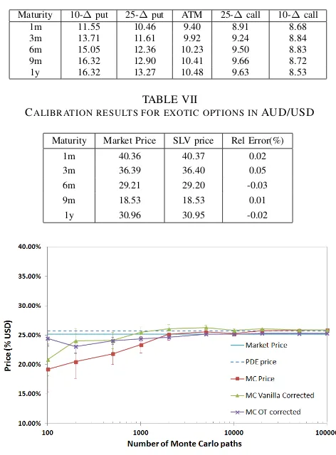
TABLE VI
CALIBRATED IMPLIED VOLATILITY SURFACE FROM THESLVFOR AUD/USD (IN%)
Maturity 10-∆put 25-∆put ATM 25-∆call 10-∆call
1m 11.55 10.46 9.40 8.91 8.68
3m 13.71 11.61 9.92 9.24 8.84
6m 15.05 12.36 10.23 9.50 8.83
9m 16.32 12.90 10.41 9.66 8.72
1y 16.32 13.27 10.48 9.63 8.53
TABLE VII
CALIBRATION RESULTS FOR EXOTIC OPTIONS INAUD/USD
Maturity Market Price SLV price Rel Error(%)
1m 40.36 40.37 0.02
3m 36.39 36.40 0.05
6m 29.21 29.20 -0.03
9m 18.53 18.53 0.01
[image:4.595.308.545.514.659.2]1y 30.96 30.95 -0.02
Fig. 1. The price of a one-touch option with a maturity of one year and a low barrier placed at 0.8 as a function of Monte Carlo paths. The price obtained from solving the pricing PDE is denoted by a dark blue dashed line while the market price is denoted by the light blue solid line. The red square markers indicate the raw Monte Carlo price, the green triangular markers indicate the price when a vanilla price is used as a control variate, and the purple crosses indicate where another one-touch option was used as the control variate. The connecting lines are guides to the eye. The error bars display the standard error on the price as calculated from the Monte Carlo samples.
B. Monte Carlo Results
Once the stochastic parameters and the leverage function are known, we can price other exotic options with our Monte Carlo engine using the calibrated SLV model. We choose to price two one-touch options with a one year maturity; one with a low barrier placed at 0.8, which has a market price of
25.14% of the domestic currency (USD), the other with a low barrier placed at 0.85, with a market price of 45.92%. We will compare the performance of the simple (or raw) Monte Carlo pricing method with that of the control variate scheme for the two exotic options. We implement the control variate scheme using two different types of options as the control: a). a vanilla option and b). a one-touch option with a low barrier placed at 0.01 larger than the target exotic option. Each of the control options are of the same one-year maturity as that of the target exotic option. The control one-touch options have market prices of 28.26% for the barrier placed at 0.81, and 51.94% for the barrier placed at 0.86.
Our pricing results for the one-touch option with a low barrier placed at 0.8 are presented in Figure 1. The light blue solid line indicates the market price of the exotic option. As a benchmark, we also priced the one-touch option using our PDE finite difference pricing engine, resulting in a price of 25.71%, as shown in Figure 1 by the dark blue dashed line. We then use the Monte Carlo pricing engine to price the one-touch option with a varying number of Monte Carlo paths, ranging from 100 to 100000.
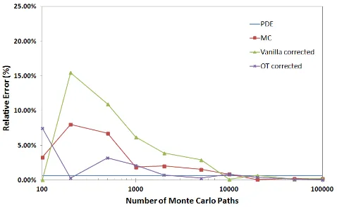
[image:5.595.307.546.53.201.2]Without using a control variate approach, we see that the Monte Carlo price indicated by the red square symbols in Figure 1 is inaccurate and exhibits a significant standard error until 10000 sample paths. The price obtained from the raw Monte Carlo method then converges to the finite difference benchmark for sample path numbers of above 10000. This behaviour is more evident when examining the absolute value of the relative error between the SLV price and the market price of the one-touch option, as presented in Figure 2.
Introducing as a control variate the corresponding vanilla option, we observe an upwards shift of the option price with reduced standard error, as shown by the green triangular markers in Figure 1 and corresponding green error bars. Furthermore, we observe an improved pricing performance for sample numbers between 200 and 2000 with a reduction in the relative error as shown in Figure 2. The vanilla-controlled price then converges to the raw MC result as the sample path number increases. The control variate scheme therefore results in faster convergence to the SLV solution which we assume here to be the PDE solution as the benchmark for the SLV model.
The pricing results for the second control variate scheme are indicated by the purple crosses in both Figure 1 and Fig-ure 2. As we are using an option with the same payout and a very similar trigger level as a control, the correlation between the control and the target will be significantly larger than the correlation between the target and its corresponding vanilla option. Therefore, from Equation (14), we would expect the standard error to be less than the vanilla-controlled result. Indeed, that is what we observe – the prices obtained from using a one-touch option as a control exhibits significantly smaller standard error than either the raw Monte Carlo or the vanilla-controlled results.
However, we observe that the one-touch controlled price
Fig. 3. The price of a one-touch option with a maturity of one year and a low barrier placed at 0.85 as a function of Monte Carlo paths. The error bars display the standard error on the price as calculated from the Monte Carlo samples. The different pricing techniques are represented by the same coloured symbols as in Figure 1.
Fig. 4. The absolute value of the relative error of the price of a one-touch option with a maturity of one year and a low barrier placed at 0.85 as a function of Monte Carlo paths compared to the market price. The different pricing techniques are represented by the same coloured symbols as in Figure 2.
[image:5.595.308.547.271.418.2]benchmark.
The pricing behaviour of the second exotic option with a barrier placed at 0.85 is displayed in Figures 3 and 4. Once again, using another one-touch option as a control variate enables the Monte Carlo-obtained price to converge faster than either the raw (naive) Monte-Carlo result or when using a vanilla option as the control. However, our calibrated model gives a more accurate price for this option, as can be seen in the much smaller relative error of the PDE benchmark price. Therefore, little extra market information is gained when using an additional exotic option as a control, and all prices converge to a uniform value for very large numbers of sample paths.
IV. CONCLUSION
We have implemented a Monte Carlo pricing engine for our hybrid stochastic-local volatility (SLV) model which can reproduce market implied volatilities and be used to price various types of exotic options. We have also evaluated the improvements in accuracy generated by using a control variate scheme to reduce Monte-Carlo sample variance. In particular, numerical results suggest that using available market-traded exotic options as control variates is preferable to using a vanilla option when pricing exotic options. The reason for such improvement in accuracy is probably due to some extra market information contained by the exotic option prices used as the control. The potential for the inclusion of additional market information gives such Monte-Carlo methods the advantage over standard PDE benchmark solutions in pricing exotic options more aligned with market prices.
ACKNOWLEDGMENT
We thank Julian Cook from FENICS for providing the AUD/USD market data, and for the insightful discussions and valuable feedback.
REFERENCES
[1] Y. Ren, D. Madan, and M. Q. Qian, “Calibrating and pricing with embedded local volatility models,” Risk, pp. 138–143, September 2007.
[2] G. Tataru and T. Fisher, “Stochastic local volatility,” 2010, Bloomberg. [3] I. J. Clark,Foreign Exchange Option Pricing: A Practitioners Guide.
West Sussex: John Wiley & Sons, 2011.
[4] G. Tataru, T. Fisher, and J. Yiu, “The bloomberg stochastic local volatility model for fx exotics,” 2012.
[5] B. Dupire, “Pricing with a smile,”Risk, pp. 18–20, January 1994. [6] P. Henry-Labord`ere, “Calibration of local stochastic volatility models
to market smiles,”Risk, no. September, pp. 112–117, 2009. [7] Y. Tian, Z. Zhu, F. Klebaner, and K. Hamza, “Calibrating and
pricing with stochastic-local volatility model,” 2012, working paper. http://http://ssrn.com/abstract=2182411.
[8] I. Gy¨ongy, “Mimicking the one-dimensional marginal distributions of processes having an Ito differential,”Probability Theory and Related Fields, vol. 71, pp. 501–516, 1986.
[9] E. Derman and I. Kani, “The volatility smile and its implied tree,”
Goldman Sachs Quantitative Strategies Research Notes, January 1994. [10] Y. Tian, “The hybrid stochastic-local volatility model with applications in pricing FX options,” Ph.D. dissertation, Monash University, 2013. [11] K. J. in’t Hout and S. Foulson, “ADI finite difference schemes for option pricing in the Heston model with correlation,”International Journal of Numerical Analysis and Modeling, vol. 7, no. 2, pp. 303– 320, 2010.
[12] D. Tavella and C. Randall,Pricing Financial Instruments: The Finite Difference Method. New York: John Wiley & Sons, 2000. [13] A. L. Lewis, Option Valuation Under Stochastic Volatility: With
Mathematica Code. California: Finance Press, 2000.
[14] D. Tavella, Quantitative Methods in Derivatives Pricing: An Intro-duction to Computational Finance. Hoboken: John Wiley & Sons, 2002.
[15] T. Kluge, “Pricing derivatives in stochastic volatility models using the finitedifference method,” Ph.D. dissertation, Chemnitz Technical University, 2002.
[16] D. J. Duffy,Finite Difference Methods In Financial Engineering: A Partial Differential Equation Approach. West Sussex: John Wiley & Sons, 2006.
[17] G. Winkler, T. Apel, U. Wystup, and N. M. Strasse,Foreign Exchange Risk: Models, Instruments and Strategies. London: Risk Books, 2007, ch. Valuation of Options in Heston’s Stochastic Volatility Model Using Finite Element Methods, pp. 283–303.
[18] S. Heston and G. Zhou, “On the rate of convergence of discrete-time contingent claims,”Mathematical Finance, vol. 10, no. 1, pp. 53–75, 2000.