Evaluating Soil Water Content Data Monitored at Different Locations in a Vineyard with Regard to Irrigation Control

Evaluating Soil Water Content Data Monitored at Different

Locations in a Vineyard with Regard to Irrigation Control

Reinhard NOLZ* and Willibald LOISKANDL

Institute of Hydraulics and Rural Water Management, Department of Water, Atmosphere and Environment, University of Natural Resources and Life Sciences, Vienna, Austria

*Corresponding author: [email protected]

Abstract

Nolz R., Loiskandl W. (2017): Evaluating soil water content data monitored at different locations in a vineyard with regard to irrigation control. Soil & Water Res., 12: 152−160.

Knowledge on the water content of a certain soil profile and its temporal changes due to rainfall and plant water uptake is a key issue for irrigation management. In this regard, sensors can be utilized to monitor soil water content (SWC). Due to the characteristic spatial variability of SWC, a key question is whether the measurements are representative and reliable. This study focused on the assessment of SWC and its variability in a vineyard with subsurface drip irrigation. SWC was measured in profiles down to a 50 cm depth by means of multi-sensor capacitance probes. The probes were installed at six locations along vine rows. A temporal stability analysis was performed to evaluate the representativeness and reliability of each monitoring profile with regard to irrigation control. Mean SWC was within a plausible range compared to unsaturated hydraulic parameters determined in a laboratory. The measurements revealed a considerable variability, but standard deviations were comparable to values from literature. The main finding was that some monitoring profiles (probes) proved to be more suit-able to monitor SWC with respect to irrigation control than the others. Considering temporal stability provided helpful insights into the spatio-temporal variability of SWC measurements. However, not all questions that are related to the concept of temporal stability could be answered based on the given dataset.

Keywords: capacitance sensors; spatio-temporal variability; subsurface drip irrigation; temporal stability

Monitoring the water content of a certain soil profile provides continuous information about water storage and its temporal changes due to rainfall and plant water uptake. Such data, measured for example by means of multi-sensor capacitance probes, can help control irrigation based on soil water depletion (e.g. Thompson et al. 2007a, b; Nolz et al. 2016a). When soil water is determined by means of sen-sors, a fundamental issue is the characteristic spatial variability of soil moisture due to soil heterogeneity, vegetation, topography, and atmospheric processes (Starr 2005; Vereecken et al. 2007). Since water content is typically sensed in the immediate vicinity of a sensor, the key question is whether the meas-urements represent the (mean) water content of the surrounding area, or whether they rather reflect a relatively dry or wet spot. Such information is

sen-sors. Sources that cannot be controlled by the user include internal variability of the instrument (e.g. electronic noise), interference from soil properties (e.g. bulk electrical conductivity), and interactions between the sensing system and soil properties at a scale smaller than the sensed volume (Evett et al. 2009). In order to reduce uncertainties and to obtain reliable data, it is recommended to install several probes. The required quantity depends on the sensor type, the soil conditions, and the desired precision (Evett et al. 2012). However, for practi-cal applications it is hardly feasible to install more than a few probes.

When interpreting data or evaluating a sensor arrangement with regard to a certain purpose such as irrigation management, it might be useful to con-sider variability by selecting datasets or monitoring locations that proved to be both representative and reliable. Van Pelt and Wierenga (2001), for in-stance, indicated that permanently measuring mat-ric potential in as few as one or two proper places is an option to automatize irrigation management based on the sensor data. They applied a temporal stability concept and concluded that this can be a powerful technique for soil water management. Temporal stability refers to the phenomenon that, when soil water content is monitored across an area, it is usually the case that sites can be detected where soil is consistently wetter or drier than the average (Pachepsky et al. 2005; Vanderlinden et al. 2012). The basic principle is that the pattern of spatial variability is more stable over time than would be expected from random processes. While hydrologists typically use the concept on a large (catchment) scale (e.g. Famiglietti et al. 2008; Mittelbac & Seneviratne 2012), it is interesting that the phenomenon can be observed at different scales, for instance also on field scale (e.g. Evett et al. 2009). Some studies focused on near-surface soil moisture, others addressed the variability down a soil profile (Pachepsky et al. 2005; De Lannoy et al. 2006; Bogena et al. 2010). However, it has to be noted that temporal stability of soil water content is influenced by environmental conditions that might change with time – e.g. soil (hydraulic) properties, vegetation, weather, and interrelations only little known so far (Vanderlinden et al. 2012).

The spatio-temporal variability of soil water con-tent in a subsurface drip irrigated vineyard – as described by Nolz et al. (2016b) – raised several questions with regard to soil water monitoring and

data interpretation as the basis for irrigation manage-ment. This subsequent study is based on profile water contents that were monitored in selected locations along vine rows. The main objectives were (i) to as-sess soil water content and its variability, and (ii) to evaluate representativeness and reliability of each monitoring profile with regard to irrigation control. Specific research questions were: Which probe is the most representative and reliable? Which probe is the best to decide upon the control (on and off ) of the subsurface drip irrigation system? For this purpose, the temporal stability of soil water content data was analyzed on a monthly basis to better il-lustrate changes over time. In order to consider also the effects from plant water uptake and irrigation, the data were separated into vegetation periods with irrigation, vegetation periods without irrigation, and non-vegetation periods.

MATERIAL AND METHODS

determined by means of a pressure plate apparatus were: water content at field capacity = 0.27 cm3_/cm3 (at a matric potential of −33 kPa), water content at permanent wilting point = 0.14 cm3_/cm3 _{(at a matric} potential of −1.5 MPa).

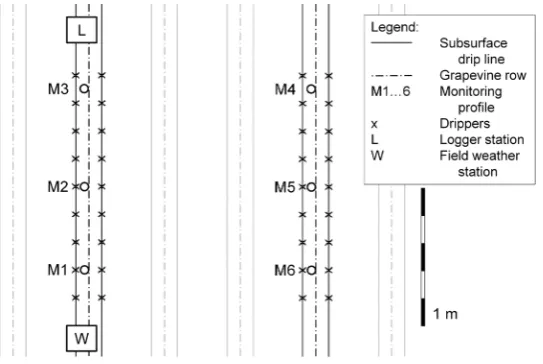
Soil water content monitoring. EnviroSCAN® _soil

moisture sensors (Sentek Pty Ltd., Stepney, Australia) were utilized for this study. Six PVC plastic access tubes were installed vertically at a lateral distance of 20 cm to the respective vine row, which promised to encounter the rooting zone (installation directly in the row was impractical as the tensioning wires restricted handling). Three tubes were in the second and three in the fifth of six rows that represented the study plot (Figure 1). The installation was executed according to the manufacturer’s best management practice recommendations using an original toolkit. The procedure guaranteed a tight contact between the access tubes and the surrounding soil. The monitor-ing profiles were numbered M1–M6. M1, M2, M5, and M6 were placed very next to a dripper; M3 and M4 were installed between two drip emitters along the drip line in order to obtain information about the horizontal expansion of the irrigation water front along the drip lines. Each EnviroSCAN probe contained five sensors on a mounting rail that was inserted into the respective access tube to measure water content at 10, 20, 30, 40, and 50 cm down the soil profile. The depths represent the central depth of measurement, the depth range of the measuring field of a single sensor is usually given with 10 cm (in natural conditions it depends on the water content). The capacitance sensors work with a so-called Frequency Domain Resonance principle (FDR), where an electromagnetic oscillation is induced in a certain volume of soil, and the frequency of oscillation is

proportional to the ratio of air and water in the soil (Paltineanu & Starr 1997). Sensor readings were converted to Scaled Frequency values SF = (F_a – F_s)/ (F_a – F_w). F_a and F_w were determined in the labora-tory as sensor-specific frequency reading in air and in water, respectively. F_s is the frequency reading in the moist soil in the field. Sensed soil water content (SWC) was calculated by means of the standard calibration relationship SF = 0.1957·SWC 0.4040 _{+ 0.0285 for sands,} loams, and clay loams (Sentek 2001). For this study, the default calibration was assumed to be adequate as mainly comparative analyses were considered. Perform-ing a site-specific calibration is a destructive process that also depends on the soil moisture conditions, which cannot be controlled easily in natural condi-tions. Generally, calibrations for EnviroSCAN sensors can vary depending on soil type, bulk density, and bulk electrical conductivity (Evett et al. 2009).

SWC data were stored in hourly intervals (or shorter) on a Sentek RT6-Logger (Sentek Pty Ltd., Stepney, Australia) and regularly downloaded on a notebook. Data from June 2010 to December 2013 were used for this study. SWC is defined as volume of water per volume of soil (cm3_/cm3_{). In this work,} sensor data are expressed as percentage, which is equivalent to (cm3_/cm3_{) × 100. It can also be} inter-preted as mm·(100 mm)−1_{, which then represents the} water height in a soil profile of 100 mm (as the sen-sors are mounted at a 10 cm distance, a 10 cm deep soil layer is related to each sensor). SWC of a profile was calculated as the average of sensor readings at five depths. Hence, the SWC values presented and discussed later in this article represent the integrated profile water content (in %).

Temporal stability analysis. Temporal stability of SWC was determined using the mean relative

ence technique (Vachaud et al. 1985; Vanderlinden et al. 2012). In doing so, the relative difference RD_ij for location i and time j was calculated as

(1)

where:

SWC_ij – sensed water content at location i (i = 1–6 for the six probes) and time j (daily average)

<

>

The mean relative difference (MRD) for location i is then

(2)

where:

N_t – number of observation terms (e.g. days of a month)

The corresponding standard deviation (SDRD) was calculated according to Jacobs et al. (2004) as

(3)

Any location with an MRD_i near to zero is usually considered representative throughout time (Vachaud et al. 1985; Pachepsky et al. 2005). Furthermore, also small SDRD_i values reflect temporal stability as, for example, a location with a small SDRD_i and an offset can easily be transformed to obtain average values (Vanderlinden et al. 2012). In order to consider both values for data interpretation, a so-called root mean square error (RMSE) was calculated as

. ₍₄₎

Any location i with the smallest RMSE_i was con-sidered as the most representative one. For a better readability, indices are omitted when the reference location is obvious.

RESULTS AND DISCUSSION

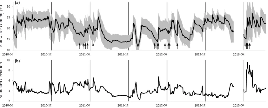
Assessment of soil water content data and their variability. After installation of the probes in June 2010, there was a short drying phase until a large rainfall event (31 mm) on July 15 (Figure 2). After that, frequently occurring rainfall kept the soil in an untypically moist status throughout the vegetation period, represented by a sensed profile water content of about 24% on average (Figure 2a). SD was relatively constant during this moist period; its mean was ± 4.2% (Figure 2b). As SD is related to precision in general, a smaller SD of replicate values can be interpreted as a greater precision with which the mean value is known. The vineyard was not irrigated in 2010. In 2011, mean SWC decreased during April. Conse-quently, irrigation was applied on May 11 + 31, June 7 + 17, and July 14. The water application is reflected by increasing soil water content (Figure 2a) and cor-responding peaks of SD values (Figure 2b). The latter reflect larger differences between the probes, likely due to the application of water via point sources and its subsequent inhomogeneous distribution in the soil. From August on, mean SWC dropped to about 14% and remained at this status until January 2012

Figure 2. Mean soil water content (black line) and standard deviation (grey bars) calculated from the readings of six multi-sensor capacitance probes in 0–50 cm deep profiles; arrows indicate irrigation events (a), course of standard deviation (b)

1

1

MRDi j NtRDij

j t

N









2 1

1

SDRD (RD MRD )

1

t

j N

i ij i

j t

N





 





2 2

RMSEi MRD SDRDi  i

SWC SWC

RD

SWC

ij j

ij

j

  



 

St

and

ar

d de

vi

ation

Soil w

at

er c

on

ten

(Figure 2a). The corresponding SD values were also small (Figure 2b). Mean SD was ± 4.7% in the first half-year and ± 3.8% in the second. In January 2012, SWC increased considerably. The sudden decrease in February was mainly due to soil freezing, so these data should not be over-interpreted. From March to May, there was again a continuous decrease of SWC. Therefore, the vines were drip irrigated on April 29, May 15 + 18, June 18, July 5 + 11, and August 18. After harvest, SWC decreased until mid of October and then was increased again by natural precipita-tion (Figure 2a). Due to the changing condiprecipita-tions in 2012 – freezing, rainfall, irrigation – SD fluctuated considerably (Figure 2b). Its mean value was 3.9%. From January to March 2013 the soil was constantly wet (Figure 2a). During April, like in the previous years, SWC decreased. Unfortunately, there were gaps in SWC data from mid of May to June; mean SD was 3.4%. In July 2013, the winegrower started a substantial irrigation campaign with events on July 11, 13, 16, 17, 25, 28, and 29 (Figure 2a). At that time, SD values easily exceeded all previous values

(Fig-ure 2b), reflecting considerable differences between the locations. The details of this irrigation period will be discussed in a separate section.

In general, the mean SWC reflected both dry and moist phases during the investigated period (Fig-ure 2), representing good preconditions for further analysis. The minimum and maximum SWC was 12% and 27%, respectively. This can be characterized as typical range compared to the SWC of 14% and 27% at permanent wilting point and field capacity, respectively. However, field measured SWC seldom coincides with unsaturated hydraulic parameters determined in the lab, which is particularly the case when data from just a single probe are considered (e.g. Nolz et al. 2016a). SWC data of the six probes in this study were considerably different (Figure 2). However, the SD values are comparable to values found in literature. Evett et al. (2009), for example, measured water contents of 2-m profiles in the field using EnviroSCAN probes (n = 10). They reported mean SD values between ± 1.1% and ± 5.4%, depend-ing on soil water status, irrigation, and crop. A better

Figure 3. Soil water content in the profile (mean of five sensor readings) measured at four monitoring locations during an intensive irrigation campaign in July 2013

Soil w

at

er c

on

ten

t (%) (0−50 c

m pr

ofile)

(a) M1

(b) M3

(c) M4

precision (smaller SD values) can be obtained with more replications, implying that the mean value is known with greater certainty. However, it has to be noted that this does not necessarily entail better accuracy in terms of deviation of a measured value from the real value.

Interpretation of soil water content data of ir-rigation events. Figure 3 illustrates SWC readings of M1, M3, M4, and M6 during the period of intensive irrigation in July 2013 (M2 and M5 are not illustrated because of data gaps that occurred during this phase). At location M1, SWC likely reached saturation due to irrigation on July 17 and 25, as induced by horizontal lines at values of almost 40% (Figure 3a). In this case, irrigation was sub-optimal. M6 sensed a similar SWC; the irrigation events were reflected properly, but not the effect of the events on July 17 and 25 (Figure 3d). M3 showed no reaction to irrigation, and M4 reacted only on July 17 – after substantial irrigation – and later on July 26 (Figure 3b, c). It is evident that the laterally transported water did not reach the sensing volume of the probe at position M3, and it reached M4 with a considerabe delay (both positions were in

the mid between two emitters). The placement of a probe in relation to an emitter thus proved to have an immense effect on the measurements. M3 and M4 were neither suitable for irrigation monitoring nor for irrigation control, especially not to decide about when to stop irrigation. The dissimilarities explain the large SD values in Figure 2b.

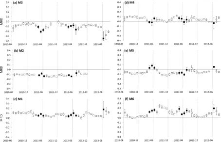
Assessment of mean relative differences over time and evaluation of locations (probes) with regard to irrigation scheduling. The monthly MRDs reveal considerable differences between non-vegeta-tion periods (October-March) and vegetanon-vegeta-tion peri-ods (April-September), which becomes particularly evident at months when the vines were drip irrigated (Figure 4). Considering only non-vegetation periods (white squares in Figure 4), the MRDs were relatively stable during the study period. The only exceptions were the large values of the M6 probe at the end of 2011, which cannot be explained based on the existing data. In contrast to non-vegetation periods, MRDs of months with irrigation events (black squares in Figure 4) deviated considerably from the mean. The largest differences were found in July 2013, when

several irrigation events were initiated (as illustrated in Figure 3). Consequently, SDRD values were the largest, indicating substantial differences between the measurements at locations next to emitters (M1, M2, M5, and M6) and probes at a 0.5 m distance from the emitters (M3 and M4) (Figure 4). Evidently, the differences between non-vegetation and vegetation

periods can be assigned to heterogeneous soil water distribution due to subsurface drip irrigation. This indicates that the relative differences technique can help evaluating locations for soil water monitoring with a view to irrigation control. For example, SWC was overrepresented by M1 (in relation to the aver-age), whereas M3 delivered too small values (Figure 4). On the other hand, the concept reaches its limits considering irrigation periods, because a merely statistical approach might not be suitable anymore when considerable physical differences appear due to the application of irrigation water from point sources and subsequent inhomogeneous distribu-tion in the soil. For an unbiased temporal stability analysis, it is recommended to consider such effects when installing soil water sensors. For instance, a random setup might deliver interesting data.

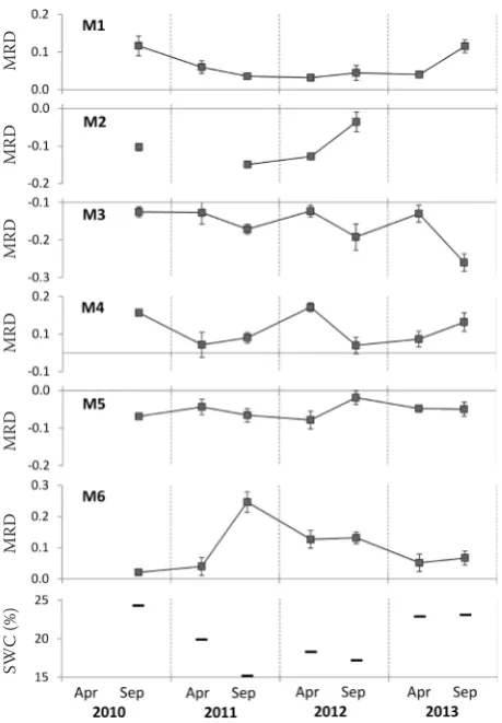
In order to evaluate if temporal stability is affected by moisture conditions or changes over time, the MRD values with SDRD of April and September and the corresponding mean SWC were considered (Figure 5). These two months were selected, because they were counted to the vegetation period but not affected by irrigation events. The main outcome is that the data revealed no evident systematic re-lationships, neither regarding different moisture conditions nor regarding development over time (Figure 5). Unfortunately, missing data (M2) as well as unexplainable large values (M6, September 2011) influenced the MRD values of the respective months. As the number of probes and their arrangement was mainly fixed with regard to irrigation management, the setup was evidently not sufficient to draw reliable conclusions regarding dynamic developments (for example, such as induced by plant development), although the underlying data series was longer than in other investigations presented in literature.

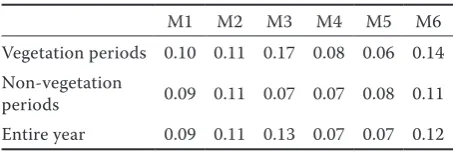
To decide which location and accordingly which probe was the best to monitor soil water content with respect to irrigation scheduling, MRD values of the study period were separated into vegetation and non-vegetation periods (Figure 6). Furthermore, cor-responding RMSE_i values were calculated to evaluate temporal stability numerically by considering both MRD_i and SDRD_i values (Table 1). The selection of an adequate probe turned out to depend strongly on the point of view. With a focus on the entire year, it is evident that M4 and M5 performed best according to the temporal stability analysis, followed by M1, M2, M6, and M3 (Table 1). The latter, however, to-gether with M4 had the smallest RMSE_i value during

Figure 6. Mean relative difference (MRD) with respective standard deviations (SDRD; error bars) for vegetation pe-riods, non-vegetation pepe-riods, and entire years

Figure 5. Mean relative difference (MRD) with respective standard deviations (SDRD; error bars) of the six locations and mean monthly soil water content (SWC) of April and September (no irrigation)

S

WC (%) MR

D MR

D MR

D MR

D MR

D MR

non-vegetation periods. Hence, both locations M3 and M4 were representative as long as there was no irrigation. Considering the MRD values, M3 meas-urements were generally below the average SWC, whereas M4 measurements were above the average (Figure 6). Regarding the decreasing SWC values that were observed in springtime of all years (Figure 2), M3 would be the best choice as the basis for irriga-tion scheduling in order to avoid water deficit stress. However, it would be a proper choice only from this particular point of view. MRD values of M5 were closest to zero during vegetation periods (Figure 6) and RMSE_i was the smallest (Table 1). Accordingly, M5 would be the best choice for soil water moni-toring in general. It was already mentioned that the mean SWC corresponded well with the unsaturated hydraulic parameters determined in the lab. Con-sequently, M5 is likely the best choice to schedule irrigation based on the management allowed depletion of soil water (e.g., Nolz et al. 2016a). M4 performed second best, although the sensor readings did not reflect irrigation (Figure 2). M1 returned moderate RMSE_i values compared to the other locations (Ta-ble 1) and represented a rather wet spot according to the MRD values (Figure 6). Hence, M1 might be a helpful monitoring location to avoid over-irrigation as illustrated in Figure 3. Within the given setup, M2 and M6 were the least useful.

CONCLUSIONS

The study focused on the assessment of profile water content, measured down to a 50 cm depth by six capacitance probes at selected positions along vine rows, and its variability. Mean soil water content was within a plausible range compared to unsaturated hydraulic parameters determined in a laboratory. The measurements revealed a considerable variability, but standard deviations were comparable to values from literature. The representativeness and reliability of each monitoring profile was evaluated with regard

to irrigation control. For this purpose, temporal stability was assessed by determining mean relative differences and corresponding standard deviations for different periods. The main finding was that some positions (probes) were more suitable for soil water monitoring with respect to irrigation control than the others. In the given case, a single location proved to be most suitable for this purpose. Furthermore, data from three others could serve as the basis for irrigation scheduling with some restrictions, while two locations were not useful.

Altogether, the results provided helpful insights into the spatio-temporal variability of soil water content measurements and allowed to evaluate the monitoring locations (and probes). The most critical reflection is that a substantial uncertainty remains if only one or two probes are installed. However, this might be a typi-cal case due to practitypi-cal and economic reasons. Other conclusions concern the temporal stability analysis. In general, it proved to be a useful tool to answer the research questions. On the other hand, interpretation was not always straightforward as the resulting recom-mendations depended on the focus, for example, if and in which way irrigation was considered. Furthermore, the available data from the specific arrangement of the probes were not suitable to assess all influences and uncertainties that might have affected temporal changes, for instance, due to plant development.

Acknowledgements. We want to thank Mr. F. Forster, Mr. K. Haigner, Ing. W. Sokol, and DI M. Wolf for their work in the field and in the lab, and Mr. M. Wahrmann who allowed us to install sensors in his vineyard. The installation of the soil water probes was partly funded by the Austrian Research Promotion Agency (FFG) in the frame of the pro-ject Innovative approaches to the subsurface drip irrigation principle (SINAPSIS, PN822826). Names of products and companies are only mentioned for better understanding; none of the authors is in a dependency to any of the mentioned companies. Furthermore, we appreciate the work done by the reviewers and we are thankful for the comments that helped us improve the manuscript.

References

Bogena H.R., Herbst M., Huisman J.A., Rosenbaum U., Weuthen A., Vereecken H. (2010): Potential of wireless sensor networks for measuring soil water content vari-ability. Vadose Zone Journal, 9: 1002–1013.

Celette F., Gaudin R., Gary C. (2008): Spatial and temporal changes to the water regime of a Mediterranean vineyard

Table 1. Root mean square error (RMSE_i) values corre-sponding to Figure 6

M1 M2 M3 M4 M5 M6 Vegetation periods 0.10 0.11 0.17 0.08 0.06 0.14 Non-vegetation

periods 0.09 0.11 0.07 0.07 0.08 0.11

Entire year 0.09 0.11 0.13 0.07 0.07 0.12

due to the adoption of cover cropping. European Journal of Agronomy, 29: 153–162.

Dabach S., Shani U., Lazarovitch N. (2015): Optimal ten-siometer placement for high-frequency subsurface drip irrigation management in heterogeneous soils. Agricul-tural Water Management, 152: 91–98.

De Lannoy G.J.M., Verhoest N.E.C., Houser P.R., Gish T.J., Van Meirvenne M. (2006): Spatial and temporal charac-teristics of soil moisture in an intensively monitored

agri-cultural field (OPE3_{). Journal of Hydrology, 331: 719–730.}

Evett S.R., Schwartz R.C., Tolk J.A., Howell T.A. (2009): Soil profile water content determination: Spatiotemporal variability of electromagnetic and neutron probe sensors in access tubes. Vadose Zone Journal, 8: 926–941. Evett S.R., Schwartz R.C., Casanova J.J., Heng L.K. (2012):

Soil water sensing for water balance, ET and WUE. Ag-ricultural Water Management, 104: 1–9.

Famiglietti J.S., Ryu D., Berg A.A., Rodell M., Jackson T.J. (2008): Field observations of soil moisture variability across scales. Water Resources Research, 44: W01423. Jacobs J.M., Mohanty B.P., Hsu E., Miller D. (2004): SMEX02:

Field scale variability, time stability and similarity of soil moisture. Remote Sensing of Environment, 92: 436–446. Medrano H., Tomás M., Martorell S., Escalona J.M., Pou A., Fuentes S., Flexas J., Bota J. (2015): Improving water use efficiency of vineyards in semiarid regions: A review. Agronomy for Sustainable Development, 35: 499–517. Mittelbach H., Seneviratne S.I. (2012): A new perspective on

the spatio-temporal variability of soil moisture: temporal dynamics versus time-invariant contributions. Hydrology and Earth System Sciences, 16: 2169–2179.

Nolz R., Cepuder P., Balas J., Loiskandl W. (2016a): Soil water monitoring in a vineyard and assessment of un-saturated hydraulic parameters as thresholds for irriga-tion management. Agricultural Water Management, 164: 235–242.

Nolz R., Loiskandl W., Kammerer G., Himmelbauer M.L. (2016b): Survey of soil water distribution in a vineyard and implications for subsurface drip irrigation control. Soil and Water Research, 11: 250−258.

Pachepsky Y.A., Guber A.K., Jacques D. (2005): Tempo-ral persistence in vertical distribution of soil moisture

contents. Soil Science Society of America Journal, 69: 347–352.

Paltineanu I.C., Starr J.L. (1997): Real-time soil water dy-namics using multisensor capacitance probes: laboratory calibration. Soil Science Society of America Journal, 61: 1576–1585.

Sentek (2001): Calibration of Sentek Pty Ltd Soil Moisture Sensors. Manual, 60 pp.

Starr G.C. (2005): Assessing temporal stability and spatial variability of soil water patterns with implications for precision water management. Agricultural Water Man-agement, 72: 223–243.

Thompson R.B., Gallardo M., Valdez L.C., Fernandez M.D. (2007a): Using plant water status to define threshold val-ues for irrigation management of vegetable crops using soil moisture sensors. Agricultural Water Management, 88: 147–158.

Thompson R.B., Gallardo M., Valdez L.C., Fernandez M.D. (2007b): Determination of lower limits for irrigation man-agement using in situ assessments of apparent crop water uptake made with volumetric soil water content sensors. Agricultural Water Management, 92: 13–28.

Vachaud G., Passerat De Silans A., Balabanis P., Vauclin M. (1985): Temporal stability of spatially measured soil wa-ter probability density functions. Soil Science Society of America Journal, 49: 822–828.

Van Pelt R.S., Wierenga P.J. (2001): Temporal stability of spatially measured soil matric potential probability den-sity function. Soil Science Society of America Journal, 65: 668–677.

Vanderlinden K., Vereecken H., Hardelauf H., Herbst M., Martinez G., Cosh M., Pachepsky Y. (2012): Temporal stability of soil water contents: A review of data and analyses. Vadose Zone Journal, doi 10.2136/vzj2011.0178 Vereecken H., Kamai T., Harter T., Kasteel R., Hopmans J., Vanderborght J. (2007): Explaining soil moisture vari-ability as a function of mean soil moisture: A stochastic unsaturated flow perspective. Geophysical Research Let-ters, 34: L22402.