Explicit Substitution and Sorted Bigraphs
A dissertation submitted to the
University of Dublin, Trinity College
for the degree ofDoctor of Philosophy
Shane Thomas Ó Conchúir
Department of Computer Science University of Dublin, Trinity CollegeIreland
Declaration
This thesis has not been submitted as an exercise for a degree at any other university. Except where otherwise stated the work described herein has been carried out by the author alone.
This thesis may be borrowed or copied upon request with the permission of the Librarian, Univer-sity of Dublin, Trinity College. The copyright belongs jointly to the UniverUniver-sity of Dublin and the author.
Signed:
Shane Thomas Ó Conchúir
Summary
This dissertation investigates the notions of sorting and explicit substitution in the framework of bigraphs. We present kind sortings which endeavour to add enough structure to bigraphs to allow faithful representations, within this framework, of both the nested grammar of models of formal calculi and the hierarchical structures encountered in context-aware systems and network topographies. We also explore Milner’s bigraphical representation of explicit substitutions.
Pure, or unsorted, bigraphs are composed of a linking structure and a nesting structure, both self-reconfigurable, which respectively model mobile connectivity and mobile locality. They have a rich dynamic theory but limited applications. Sortings allow bigraphs to model more significant applications. We begin by defining kind sortings which allow us to refine the nesting structure with respect to a containment relation. We proceed by enriching the nesting structure with capacities and then proving that the sorting retains the rich dynamic theory of pure bigraphs.
Applications of the sorting include: a better modelling of formal calculi with a sorted, ordered grammar with capacities e.g. the λ-calculus; an interpretation of basic types as sets of controls and of a type preorder as subset inclusion, allowing us to present bigraphical models of typed λ-calculi; the introduction of basic flow control for the reaction relation, allowing us to express simple algorithms; and an encoding of semi-structured data with an ordered tree structure and capacitiese.g. XML data and contexts.
Milner’s bigraphical encoding of his λ-calculus of explicit substitutions is indirectly studied. We contrast its notion of non-local substitution with the local substitution found in most explicit substitution (ES) calculi. We investigate properties of Milner’s calculus and discover that it satisfies many desirable properties of ES calculi. The set of properties it satisfiese.g. open confluence, full composition of substitutions, and preservation of strong normalisation, holds for few of these calculi. We attribute its properties to the non-local method of substitution which arises naturally from the bigraphical model. We present proofs of normalisation based on a novel simulation of non-local substitution with local substitution and characterise the set of strongly normalising terms of the calculus using an intersection type system.
Explicit Substitution and Sorted Bigraphs
Approved by
For Dad,
Contents
Summary iii
Acknowledgements xix
Chapter 1 Introduction 1
1.1 Contributions of the thesis . . . 8
1.2 Hypotheses . . . 9
1.3 Structure of the dissertation . . . 10
Chapter 2 Concepts and Terminology 12 2.1 Preliminary notation . . . 13
2.2 Category Theory . . . 14
2.3 Pure bigraphs . . . 21
2.3.1 Place graphs . . . 25
2.3.2 Link graphs . . . 26
2.3.3 Bigraphs . . . 27
2.3.4 Related work . . . 32
2.4 Term rewriting systems . . . 32
2.5 Theλ-calculus . . . 35
2.6 Explicit substitutions . . . 36
2.7 Type Systems . . . 39
I
Kind Sorted Bigraphs
42
Chapter 3 Kind Bigraphs 44 3.1 Introduction . . . 443.2 Place sorting . . . 50
3.3 Fundamental kind sorting . . . 51
3.4 Kind sorting with visibility . . . 54
3.5 Kind sortings with maximum capacities . . . 57
3.6 Kind sorting with min-max capacities . . . 63
3.6.1 Problems with kind sorting with capacities . . . 67
3.7 Conclusions . . . 68
3.8 Further work . . . 69
Chapter 4 Static Theory 71 4.1 Basic properties . . . 71
4.1.1 Hard bigraphs . . . 73
4.2 Further properties . . . 75
4.2.1 Operations and decompositions . . . 78
4.3 Subcategories of kind sortings . . . 80
4.4 Conclusions . . . 85
4.5 Related work . . . 86
Chapter 5 Transition Theory 87 5.1 Transfer of dynamic theory . . . 88
5.2 Basic properties . . . 94
5.3 Relative pushout creation . . . 95
5.3.1 Relative pushouts for kind sortings . . . 96
5.3.2 Relative pushouts for subcategories of kind sortings . . . 97
5.4 Pushout reflection . . . 99
5.4.1 Pushout reflection for kind sortings . . . 99
5.4.2 Pushout reflection for subcategories of kind sortings . . . 99
5.5 Conclusions . . . 100
5.5.1 Related work . . . 103
Chapter 6 Further Sortings 104 6.1 Place sortings . . . 105
6.1.1 Deep kind sorting . . . 105
6.1.2 Deep sorting with capacities . . . 107
6.2.1 Definitions . . . 109
6.2.2 Tiled link sorting . . . 110
6.2.3 Plain sorting . . . 112
6.3 Compound sortings . . . 115
6.3.1 Combining sortings . . . 115
6.3.2 Kind rigid control-sorting with visibility . . . 117
6.4 Summary . . . 119
6.5 Related work . . . 119
II
Milner’s
Λ
subCalculus
122
Chapter 7 λ-calculi with Explicit Substitution 124 7.1 Introduction . . . 1247.2 The calculi under discussion . . . 125
7.2.1 Theλxgccalculus . . . 125
7.2.2 λlxr . . . 126
7.2.3 λes . . . 130
7.2.4 Λsub . . . 131
7.2.5 ComparingΛsubandλxgc . . . 132
7.2.6 ComparingΛsubandλlxr . . . 132
7.2.7 ComparingΛsubandλes . . . 133
7.3 PSN and composition of substitutions . . . 133
7.3.1 Weak/full composition . . . 134
7.3.2 Breaking PSN . . . 134
7.3.3 λxkc . . . 135
7.3.4 λxc. . . 136
7.3.5 λxc− . . . 137
7.3.6 λσ . . . 137
7.3.7 Λsub . . . 137
7.4 Summary and related work . . . 138
Chapter 8 Inductive Proofs 139 8.1 Proof of confluence forΛsub . . . 139
Chapter 9 Strong Normalisation 147
9.1 Simulating non-local substitution with local substitution . . . 148
9.1.1 The problems . . . 148
9.1.2 A solution . . . 149
9.1.3 First approach: altering the target calculus . . . 151
9.1.4 Second approach: a pessimistic translation . . . 152
9.1.5 Comparison between the approaches . . . 152
9.2 PSN ofΛsub via simulation inλblxr . . . 153
9.2.1 The encoding ofΛsub inλblxr. . . 153
9.2.2 The propagation calculus for the simulation . . . 155
9.2.3 Proof of PSN usingλblxr . . . 158
9.2.4 Sketch of proof of PSN by translation toΛI . . . 160
9.3 SimulatingΛsubreduction inλes . . . 161
9.4 Characterisation ofSNΛsub and a second proof of PSN . . . 164
9.4.1 Intuitions . . . 164
9.4.2 Proof outline . . . 169
9.5 Conclusions . . . 174
9.6 Related work . . . 175
III
Applications of Kind Sortings
179
Chapter 10 Expressiveness of Kind Sorting 181 10.1 Notation . . . 18210.2 In the absence of control... . . 182
10.2.1 Multiple readers . . . 182
10.2.2 Smart buildings . . . 183
10.2.3 Automatic teller machine . . . 184
10.2.4 Draughts . . . 185
10.2.5 Boolean algebra . . . 188
10.2.6 Ain’t Got No/I Got Tea . . . 190
10.3 ...be determined . . . 191
10.4 Context-aware systems . . . 193
10.5.1 “Find them and kill them” . . . 195
10.5.2 Sudoku . . . 200
10.6 Semi-structured data . . . 203
10.6.1 XML documents . . . 204
10.6.2 BibTeX files . . . 204
10.7 Conclusions . . . 207
10.7.1 Related and further work . . . 207
Chapter 11 Models ofλ-calculi 208 11.1 ′Λbig. . . 210
11.1.1 The encoding ofΛsub into′Λbig . . . 210
11.1.2 Dynamic properties . . . 211
11.2 Sorting out ′Λbig. . . 212
11.2.1 The good, the bad, and the ugly . . . 212
11.2.2 ′Λbigσλνδ-sorting . . . 213
11.3 Modelling the untypedλ-calculus . . . 215
11.3.1 The sorting for ′Λbigut . . . 215
11.3.2 Static correspondence . . . 219
11.3.3 Dynamic properties . . . 219
11.3.4 Deficiency of the sorting . . . 220
11.4 Modelling the simply typedλ-calculus . . . 221
11.4.1 The sorting for ′Λbig→. . . 221
11.4.2 Static correspondence . . . 224
11.4.3 Dynamic properties . . . 226
11.5 Modelling theλ-calculus with intersection types . . . 229
11.5.1 Bounded completeness of the type preorder . . . 229
11.5.2 The sorting for ′Λbig∩ . . . 231
11.5.3 Static correspondence . . . 236
11.5.4 Dynamic properties . . . 237
11.6 Conclusions . . . 238
11.6.1 Further work . . . 239
Conclusions
243
Chapter 12 Conclusions 245
12.1 Conclusions . . . 245
12.2 Future work . . . 246
Bibliography 250 Chapter A Appendix for Part I 1 A.1 Pure bigraphs . . . 1
A.2 Homomorphic sortings . . . 3
A.2.1 Homomorphic sortings as kind sortings . . . 3
A.2.2 Homomorphic sorting and simply typed Λsub . . . 4
A.2.3 Applicability of kind sortings . . . 5
A.3 Proofs for Section 5.2 . . . 7
A.4 Proofs for Section 5.3 . . . 10
A.5 Proofs for Section 5.4 . . . 17
A.6 Proofs for Chapter 6 . . . 19
A.6.1 Tiled link sorting . . . 19
A.6.2 Plain sorting . . . 23
A.6.3 Compound sortings . . . 23
Chapter B Appendix for Part II 26 B.1 Proofs for Section 8.1 . . . 27
B.2 PSN for subcalculi ofΛsub . . . 29
B.2.1 PSN for Λsub↓gc. . . 30
B.2.2 PSN for Λsubc♭ . . . 32
B.2.3 The problem with proving PSN forΛsub . . . 39
B.3 Proof of PSN forλblxr . . . 43
B.3.1 Proof strategy . . . 44
B.3.2 Simulation ofλblxrin λI . . . 44
B.3.3 Encoding theλ-calculus inλI andλblxr . . . 47
B.3.4 The encodingj preserves strong normalisation . . . 48
B.3.5 Proof of PSN . . . 52
B.3.7 Summary . . . 52
B.4 Simulation ofΛsubreduction inλblxr. . . 53
B.5 Simulation ofΛsubreduction inλes . . . 61
Chapter C Appendix for Part III 68 C.1 Sudoku example . . . 68
C.2 Proofs for′Λbigσλνδ-sorting . . . . 72
C.3 Comparing′Λbigto other encodings of theλ-calculus . . . . 79
C.3.1 Explicit substitutions in the π-calculus . . . 80
C.3.2 Evaluation strategies . . . 80
C.3.3 Comparingλlxrand′Λbig. . . . 81
C.4 Proofs for Chapter 11 . . . 83
C.4.1 Simply typed′Λbig. . . . 83
C.4.2 Intersection typed′Λbig . . . . 84
C.5 Typing′Λbig . . . . 86
List of Figures
1.1 Reaction rule: Theπ-calculus with summation . . . 4
2.1 A relative bound(~h, h)forf~relative to~g(left) and a relative pushout (right) . . 18
2.2 Pushouts and relative pushouts . . . 19
2.3 A nearly opcartesian arrow and a nearly jointly opcartesian cospan . . . 21
2.4 Bigraphs, place graphs, link graphs, and composition . . . 23
2.5 A bigraph reacts . . . 24
2.6 A simply typed discipline for theλ-calculus . . . 41
2.7 Systemaddλ: An additive intersection type discipline for theλ-calculus . . . 41
2.8 Systemmulλ: A multiplicative intersection type discipline for theλ-calculus . . . 41
3.1 Model: An abstract model of commuting workers. . . 47
3.2 Reaction rule: An agent moves between two rooms . . . 49
3.3 Reaction rule: An enemy eliminates an agent . . . 50
3.4 Containment graphs for kind signatures . . . 64
5.1 A labelled transitionLof an agentaderived from a redex r . . . 89
6.1 Relating deep kind sorting to the poset(P(K),⊆). . . 107
7.1 Reduction rules forλxgc . . . 126
7.2 Congruences forλlxr . . . 128
7.3 Reduction rules forλlxr . . . 128
7.4 Reduction rules forλes . . . 130
7.5 Reduction rules forΛsub . . . 131
8.1 Relationship between properties ofΛx terms . . . 145
9.2 Simulation of→bcgc-reduction inΛI . . . 160
9.3 RelatingΛsub terms withλI terms . . . 160
9.4 Reduction diagrams for simulatingΛsub inλes . . . 164
9.5 Systemaddλs: An additive intersection type discipline forλesandΛsub . . . 168
9.6 Systemmulλs: A multiplicative intersection type discipline forλesandΛsub . . . 168
10.1 Reaction rule: Multiple readers accessing a file . . . 183
10.2 Reaction rule: Lights that turn off when the last person exits the room . . . 183
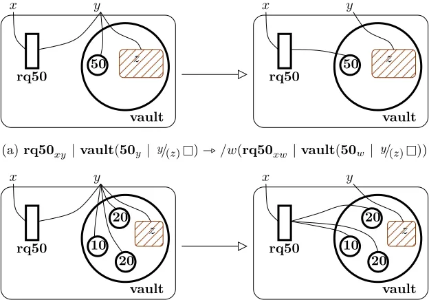
10.3 Reaction rule: The kind relation for the ATM example; The ATM returns¤50 . 184 10.4 Reaction rule: A request for¤50 is linked with notes of that value . . . 185
10.5 The kind relation for the draughts example . . . 185
10.6 Reaction rule: A hop ends (all sites contain playing pieces) . . . 186
10.7 Reaction rule: A piece is crowned . . . 187
10.8 Reaction rule: A piece advances . . . 187
10.9 Reaction rule: A player considers another move . . . 187
10.10 Reaction rule: A player takes a piece . . . 187
10.11 Reaction rule: Boolean AND . . . 189
10.12 Reaction rule: Boolean OR . . . 189
10.13 Reaction rule: Boolean IMPLIES . . . 189
10.14 Reaction rule: Boolean EQUIV . . . 189
10.15 Reaction rule: Boolean NOT and a garbage collection ‘rule’ . . . 189
10.16 The kind relation for the adventure game example . . . 190
10.17 Reaction rule: Taking and dropping items . . . 190
10.18 Reaction rule: Drop ‘no tea’ . . . 191
10.19 Reaction rule: An agent moves between two rooms . . . 192
10.20 Reaction rule: An enemy moves between two rooms . . . 192
10.21 Reaction rule: An enemy eliminates an agent . . . 192
10.22 Reaction rule: An agent collects a dot . . . 192
10.23 Kind relation for the Location-aware Printing System . . . 195
10.24 Multi-nodes for the “copy all devices” query . . . 196
10.25 Kind relation for the “copy all devices” query . . . 197
10.26 Reaction rules: The set of rules for the copy algorithm . . . 198
10.27 Example run of the flattened copy operation . . . 199
10.29 Reaction rule: Filling a square through inference . . . 202
10.30 Distributed Sudoku . . . 203
10.31 XML documents as ground kind sorted bigraphs . . . 205
10.32 An example of a kind relation for BibTeX files . . . 206
11.1 Sorting scheme for bigraphical models ofλ-calculus . . . 209
11.2 Comparing the AST of aλterm to the corresponding bigraph . . . 211
11.3 The type system for untyped′Λbig . . . 215
11.4 Two presentations of the kind sorting for′Λbig . . . 216
11.5 Ion schema for′Λbigut . . . 218
11.6 Reaction rule: Parametric reaction rule schema for′Λbigut . . . 218
11.7 Encoding of untypedΛsub terms into′Λbigut. . . 219
11.8 Typing rules for simply typedΛsub . . . 221
11.9 Representation of the simply typed′Λbig→ sorting . . . 223
11.10 Ion schema for′Λbig→ . . . 225
11.11 Reaction rule: Parametric reaction rule schema for′Λbig→ . . . 225
11.12 Encoding of simply typedΛsub terms into′Λbig→ . . . 226
11.13 Reduction cubes for′Λbig→ and′Λbig∩ . . . 228
11.14 An RPO, a join in(τ,≪), and a join in(P(K),⊆). . . 231
11.15 Ion schema for′Λbig∩ . . . 234
11.16 Reaction rule: Parametric reaction rule schema for′Λbig∩ . . . 234
11.17 Interfaces of the reaction rules . . . 235
11.18 Encoding of intersection typedΛsub terms into′Λbig∩ . . . 237
11.19 Representation of the place graph sorting of Homerσas a kind sorting . . . 242
12.1 Proposed reaction rule to model non-local substitution of metavariables . . . 248
A.1 Containment conditions of homomorphic sortings and kind sortings . . . 4
A.2 Reaction rule: Theπ-calculus with summation . . . 6
A.3 Constructing a paired sorted RPO . . . 24
A.4 Pushouts are (weakly) reflected . . . 24
B.1 The relations between theλ-calculus,λblxr, andλI . . . 45
B.2 Strong simulation of throughG . . . 51
B.4 Abbreviations in Figure B.5 . . . 55
B.5 Translation forC[(λx.v)w],xa free variable ofv . . . 55
B.6 Sets of free variables . . . 56
B.7 Abbreviations in Figure B.8 . . . 56
B.8 Translation forC[v[x/w]],xa free variable ofv . . . 56
B.9 Sets of free variables . . . 57
B.10 Abbreviations in Figure B.11 . . . 57
B.11 Translation forC[v[x/w]],xnot a free variable ofv . . . 57
B.12 Sets of free variables . . . 58
B.13 Abbreviations in Figure B.14 . . . 58
B.14 Translation forC[v[x/w]],xnot a free variable ofv . . . 58
B.15 Free variables and abbreviations for Figures B.16 and B.17 . . . 59
B.16 Translation forC1[C2[x][x/v]] . . . 59
B.17 Translation forC1[C2[v][x/v]],xa free variable ofC2[v] . . . 59
B.18 Translation forC1[C2[v][x/v]],xnot a free variable ofC2[v] . . . 59
B.19 Free variables and abbreviations for Figures B.20 and B.21 . . . 60
B.20 Translation forC[v[x/w]],xnot a free variable ofv . . . 60
B.21 Translation forC[v]. . . 60
B.22 Equations for the cases wherex /∈fv(D[u]) . . . 64
B.23 Equations for the cases wherex∈fv(D[u]) . . . 65
C.1 The initial puzzle . . . 69
C.2 The initial puzzle with marked empty squares . . . 69
C.3 Remove all marks which are not consistent . . . 70
C.4 Finish some squares and repeatedly remove marks . . . 70
C.5 After inferring what some squares must contain . . . 71
C.6 The solution . . . 71
List of Tables
5.1 Properties of kind sortings . . . 101 5.2 Proven properties of subcategories of kind sortings with visibility . . . 102
Acknowledgements
I would like to thank my supervisor, Mícheál Mac an Airchinnigh, for an inspirational, incom-parable, and unforgettable undergraduate mathematics course which raised more questions than answers (a sign of a good education) and for introducing me to category theory and bigraphs.
The core of this dissertation arose from working with Martin Elsman and Thomas Hildebrandt during a stay, kindly facilitated by Lars Birkedal and Annette Hjort Knudsen, with the Bigraphical Programming Languages group at the IT University of Copenhagen. Much of the technical work in this dissertation has its origins in that visit and conversations with the group; indeed this document may not have been written otherwise. I remain extremely grateful for the welcome I received and for the subsequent communications.
The remainder of the work presented here is largely due to the collaboration with Delia Kesner in Chapter 9 which inspired ideas in later chapters, particularly the model ofΛsubwith intersection types. I would like to thank Delia for her patience and ever-helpful comments.
Many thanks are due to Stéphane Lengrand for taking time to step through some of my technical details with me. I also wish to thank Robin Milner, Mikkel Bundgaard, Søren Debois, Kristoffer Rose, and François-Régis Sinot for their helpful correspondence and references, and others at ITU such as Rasmus Mogelberg and Troels C. Damgaard for making my stay there pleasant. This work was partially supported by the Irish Research Council for Science, Engineering, and Technology: funded by the National Development Plan.
For that, I will always be thankful. I must also thank the remaining members of the FMG with whom I had contact – Andrew, Glenn, Arthur, Hugh, Edsko (honorary member), Wendy, and Daniel – for listening to me trying to explain my work at them whilst providing a diversity of interesting topics themselves.
I owe personal debts of gratitude to Owen Conlan and my aunt Anne O’Connor who were always available with good advice on getting me through my doctorate.
And how could I not thank Mssrs. John Hamill, Alan Farrell, and David Hardy for providing me with endless buckets of beer, coffee, and abuse (in no particular order) over the years.
Most of all, I wish to thank Mum, Sinéad, and Madiha for their love, patience, and understand-ing throughout and beyond.
Shane Thomas Ó Conchúir
Chapter
1
Introduction
The scene ends badly As you might imagine
In a cavalcade of anger and fear There will be feasting and dancing In Jerusalem next year
I am going to make it through this year If it kills me
This Year – The Mountain Goats
The advent of pervasive computing has given rise to many new challenges for software engi-neers. Not only are we faced with the ubiquity of computation, the behaviour of these computa-tional devices can depend on interaction andcommunication with others, either global or local. Furthermore, the mobility of devices, processes, and communication links – whether physically or conceptually – becomes increasingly prevalent as technology becomes increasingly integral to society. Yet another challenge lies in themeans of communication; not only must we be able to reason about the process of communication, we must define how information is communicatedi.e. we must consider structured data. If we are to expect certain behaviours from these systems, or some level of security, we require analytical tools which are powerful enough to describe all of these issues.
Com-CHAPTER 1. INTRODUCTION
municating Sequential Processes (CSP) [70] and Milner’s Communicating Concurrent Systems (CCS) [99] are widely recognised as significant steps. Both theories consider the observations that can be made of a communicating system. In CSP, the behaviour of a system can be given by a set of traces, which describe the actions which have taken place. CCS considers a more refined concept ofbehavioural equivalence i.e. whether two devices appear to behave in the same manner to an external observer, by adopting Park’s notion of bisimilarity [125].
These process calculi address issues relating to inter-process communication. However, the introduction of mobile computing presents another challenge; not only can processes communicate in parallel, they can propagate through distributed systems and reconfigure their communication links. This requires more sophisticated calculi.
Milner et al.’s π-calculus [115] and the equivalent join calculus of Fournet and Gonthier [57] allow the communication of data or processes through named channels. This communication of channel names admits the concept of mobile connectivity – connections may be passed between processes. A familiar example is the passing of mobile phone connections during the hand-over pro-tocol [103]. The fusion calculus of Parrow and Victor [126] simplifies theπ-calculus and considers input and output as symmetric actions.
The movement of agents through space, ormobile locality, is a quite different form of mobility. Its importance has risen with the prevalence of both portable – perhaps context-aware – devices, which move freely through physical spaces and with mobile code propagating through virtual space. The mobile ambients of Cardelli and Gordon [32] place emphasis on hierarchical structure, mod-elling the movement of entire nested enviroments (which could represente.g. processes) through physical or virtual topologies. The distributed join calculus [57, 58] extends the join calculus with the notion of location while both the distributedπ-calculus of Sewell [139] and the Seal calculus of Vitek and Castagna [145, 35] similarly extend theπ-calculus. The treatment of mobility dif-fers among the calculi e.g mobile ambients have subjective mobility – agents move themselves – whereas the Seal calculus considers objective mobility where agents are moved by their context, for the purposes of security.
CHAPTER 1. INTRODUCTION
from which to describe and distinguish the behaviour of processes is a non-trivial problem. Process frameworks such as Milner’s action calculi [102] or Gardner and Wischik’s explicit fusions [60] address this problem by providing a common language in which to express different calculi and reason about the interactive behaviour of processes. Both frameworks are inspired by calculi with mobile connectivity. Action calculi allow various calculi to be encoded within the framework by defining a set of basic control structures and reaction rules, allowing the combination and analysis of different calculi within the same framework.
These frameworks lack two useful features. First, they do not consider the notion of locality inherent in calculi such as mobile ambients. Secondly, they do not possess a uniform treatment of labelled transitions; an LTS is defined for explicit fusions but it is provided rather than derived. Indeed, one of the aims of action calculi is to provide a general treatment of behavioural equiv-alences [102]. This work was continued by Milner in the framework ofbigraphs, which addresses both of these issues.
The bigraphs of Milner, Leifer, and Jensen [105, 91, 104, 90, 74, 73, 114] have been proposed as a framework for modelling mobile computation. Bigraphs draw on ideas from the Chemical Abstract Machine [10], interaction nets [86], Nomadic Pict [147], and the process calculi and frameworks mentioned above. Bigraphs represent both mobility of connectivity as in theπ-calculus and locality as in mobile ambients. Linkage and location are represented by two (hence ‘bi’) almost separate structures. Similar to action calculi, these structures are defined over a set ofcontrols. Mobility in a system is modelled with a set of reaction rules which describe how bigraphs in the system may reconfigure themselves, allowing many calculi and mobile systems to be modelled within the one framework.
Due to work by Leifer and Milner [91, 90], bigraphs achieve a canonical treatment of labels and behavioural equivalences1. The labelled transitions of an agent are determined purely by the reaction rules and context; the contexts themselves are used as labels. However, not all contexts should be considered as labels for both practical reasons and theoretical reasons regarding observation [140]. Leifer proposes the categorical notion of colimit, through therelative pushout universal construction, to identify a canonical set of minimal labels for a reactive system [90].
Many calculi have been encoded in the bigraphical setting; the asynchronous π-calculus [74], polyadicπ-calculus [24], and fullπ-calculus [73], theλ-calculus [111, 63], finite CCS [113], condition-event Petri nets [92], Higher-Order Mobile Embedded Resources (Homer) [22], mobile ambients [73], and the Fusion calculus [64]. Furthermore, strong correspondences have been shown syntactically,
1
CHAPTER 1. INTRODUCTION
000
000
111
111
00
00
00
11
11
11
00
00
11
11
00
00
00
11
11
11
00
00
11
11
000
000
111
111
y 0 y x 0 sum send 1 z 2 sum get 3 z 2R R′
x
sum(sendxy(0)| 1)|sum(getx(z)(2)| 3)_x| 0 | y/(z)(2)
Figure 1.1: Reaction rule for theπ-calculus with summation [74]
dynamically, and observationally – in terms of the original bisimilarity and that induced by the bigraphical mechanisms via relative pushouts – between the calculi and their encodings.
This is the starting point of our thesis. Bigraphs can express models of computation, commu-nication, and mobility however as Milner states, their pure form is not likely to support significant applications [110]. Indeed, the examples of the previous paragraph all use enriched bigraphs to allow the structure of the calculus to be reflected in both the bigraphs themselves and in the labels of the LTS. We introduce an enrichment which deals with applications the existing enrichments cannot. Before we expound on this, we informally explain the bigraphical framework.
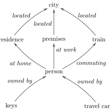
Briefly, a bigraph is analogous to a term of a process calculus or a representation of the state of some system. There are two components of a bigraph, a structure ofconnections and a structure of locations, both tied together with a set ofnodes. The first component is a hypergraph and represents publicly named or private connections between nodese.g. free/bound names of a calculus or access to some resource in a distributed system. The second component is a forest of trees, representing localitye.g. the subterm grammar of a calculus or the physical/virtual topology of some network. For example, Figure 1.1 is a visual representation of a pair of bigraphs encodingπ-calculus contexts. Thesum,get, andsendnodes in the diagram (which respectively model summation, input, and
output) are represented by labelled shapes. Locality is represented by geometric containment – the
CHAPTER 1. INTRODUCTION
Bigraphs have quite a free structure and a strong dynamic theory but the former limits its modelling power; many models and calculi have quite specific structure and grammar requiring notions like name-binding/scoping, directed links, sorting, typing, etc. Enrichments, orsortings, of bigraphs allow these notions to be added to the framework such that if the addition is careful, it can be shown using some basic category theory that the dynamic theory is retained. To date, the published literature concentrates on enriching the linking structure to allow the modelling of calculi with mobile connectivity. Enrichments of locality have not been as widely studied: Milner and Bundgaard and Hildebrandt presented sortings for finite CCS [113] and the Homer calculus [22] respectively; Birkedal et al. describe a quite general sorting of locality (discussed in Chapter 6) [15]; and Birkedal, Debois, and Hildebrandt consider sorting of both connectivity and locality based on predicates which hold for decompositions of bigraphs. [16]
This is our contribution. We presentkind sortings which enrich thelocality of bigraphs while safely retaining the dynamic theory. The fundamental kind sorting is based on a suggestion by Jensen and Milner:
Another possible refinement (of bigraphs) is a kind assigned to each node, determining the controls of the nodes it may contain. [74]
This idea forms the basis of our work. A reactive system of bigraphs is defined over a set of controls representing the basic building blocks of the system. For example, a model of the λ-calculus may use controls for the variable, abstraction, and application constructors; a model of a smart building environment may have controls representing physical locations, mobile entities, sensors, and resources. We allow the set of controls to be enriched with a relation which describes which types of control another may parent. This allows us to model, in particular, hierarchical structures like formal grammars, models reflecting the physical world, or context-aware systems with location. We also allow the specification ofcapacities e.g. that controls may contain (at most) a certain number of particular controls.
Our motivations are as follows.
Bigraphs are intended as a step towards modelling computation on a global scale. As many practical systems undergo continuous development, Milner warns against the common practice of ‘build first, analyse later.’ He advocates that in the long-term,
...system designs must be expressed from the outset with the concepts and notations of a theory rich enough to encompass all that the designers wish. [113]
CHAPTER 1. INTRODUCTION
for process calculi which respects the existing behavioural theories. Our position is that in both applications, we should strive tointernalise concepts as much as possible: a bigraphical system representing some model should only contain bigraphs whose structure agrees with the model; logical statements should be expressed in terms of bigraphical axioms rather than some external logic; analysis of thebehaviourof the system should be based on the entire system rather than some externally defined subsystem; andtype systems should be represented internally. We summarise current work in these areas and our contributions in the dissertation.
Structure Structure is crucial to modelling context-aware and distributed systems internally as these applications have strict notions of containment and capacity in general. For example, in a model of smart buildings it would be natural to express the movement of agents inside buildings rather than the movement of buildings inside agents. Kind sortings allow bigraphs to distinguish which objects may be contained inside other objects. They also allow exact and maximum capac-ities to be defined in the systeme.g. a print buffer may contain a maximum of ten pending jobs, a network contain exactly one mail server.
Published encodings of certain calculi in bigraphs are not surjective – terms of calculi are encoded into a bigraphical reactive system (Brs) where although the image of the encoding is closed under reaction, the system also contains ‘junk’ bigraphs which do not correspond to terms of the calculus2. This is true of the cited models ofλ-calculus and Homer. In the former, the grammar of theλ-calculus is not respected; aλ-abstraction may parent more than one subterm, an explicit substitution closure may not contain a body of substitution. In both models, name-binding may be malformed. Kind sortings allow us to enforce the hierarchical structure and capacity of the grammars. We also present a separate sorting which solves most of the linking problems for the λ-calculus.
For technical reasons, Milner encodes the nil CCS process as a control. However in the encoding,
0 + 0is not structurally equivalent to0. In terms of behaviour, this is not problematic as Milner recovers the bisimilarityp| nil∼pin the Brs but the structural equivalence is easily enforced if we require that each control can contain at most one nil process3.
We present kind sortings as a step towards an internal representation of locality for physical models and formal calculi in bigraphs. It subsumes the sortings of locality presented by Milner for finite CCS and by Bundgaard and Hildebrandt for Homer. Other sortings of locality, orplace
2
Our criteria allows certain bigraphs which do not correspond to terms of a calculus but which we do not consider to break the modele.gthe distribution of aπ-calculus term over many locations or the parallel composition ofλ -calculus terms. We interpret this as moving the original -calculus into a distributed or parallel setting.
3
CHAPTER 1. INTRODUCTION
sortings, have been independently studied.
The place sorting of Birkedal et al. [15] considers general relations between nodes of a bigraph and the roots of the place trees. We consider specific relations regarding containment and capacity on the more refined parent-child relation. Neither sorting generalises the other and we show in Chapter 6 that they may be safely combined.
The predicate sorting of Birkedal, Debois, and Hildebrandt subsumes many existing sortings of both locality and connectivity. It subsumes kind sortings in certain cases but in general, our sorting can not be described as a predicate sorting.
Logic Conforti, Macedonio, and Sassone [39] introduce a spatial logic in the style of Cardelli and Gordon [33] to bigraphs. Their logic is based on an axiomatisation of pure bigraphs and can express statements concerning both locality, connectivity, and dynamics.
Kind sortings provide a small contribution towards internal logics for reasoning about bigraphs. In kind sorted reaction rules, we can internally specify a certain type of precondition for reaction rules not allowed by pure bigraphs e.g. we can express reaction rules like “if a person leaves the roomand no other people remain in the room then the light switches off.” The precondition of absence in the rule is our contribution. We show how sets of such rules sometimes allow us to internally enforce some flow control to the dynamics of a system.
Semi-structured data Cardelli observes the connection between semi-structured data and mo-bile computation, particularly in the description of spatial logic [28].
Kind sorting allows models of certain semi-structured data such as XML. It admits an im-provement on the pure bigraphical interpretation of Conforti, Macedonio, and Sassone [39, 38] by allowing document order to be properly represented in the encoding, through an interpretation of Milner’s multi-nodes [111].
Behaviour The analysis of behaviour is typically based on labels of an LTS. Labels in Brssare bigraphs. A refinement of bigraphical structure then impacts the perceived behaviour. Informally, we want to restrict the contexts in which we distinguish behaviour; if the context is meaningless with respect to the intended model then observations based on the context are unhelpful. Keeping in line with our proposal for internalising analysis, we do not wish to ignore these contexts but rather prohibit them via sorting.
1.1. CONTRIBUTIONS OF THE THESIS CHAPTER 1. INTRODUCTION
between a calculus and its encoding correspond closely and is the common approach taken thus far in the bigraphical literature.
Enrichments of bigraphs should also preserve the dynamic theory of bigraphs wheree.g. bisim-ilarity is a congruence on the transition system of minimal labels. We ensure that our kind sortings do so.
Types Typing is a common feature of formal calculi and can be used to specify termination, access control policies [68], or to ensure that the right type of data is sent through a communication channel.
Kind sorting allows some notion of typing to be modelled. In the dissertation, we enrich Milner’s model of theλ-calculus with some basic type systems. We do this by interpretating types assets of typed controls. We then modeltype derivations ofλ-terms in both the simply typed and intersection typed disciplines. We do not claim that this is the ideal way to model typedλ-calculi but we use it as an example of the expressiveness of the sorting.
1.1
Contributions of the thesis
Our primary contribution is the formalisation and investigation of Jensen and Milner’s suggestion for kind sorting, repeated above. We provide definitions for different types of kind sorting; a basic sorting, a sorting with ‘hidden local structure’, and sortings which allow us to specify exact, minimum, or maximum capacities for controls. We also investigate subcategories of these sortings, one of which recovers Milner’s sorting for finite CCS. We prove that many of these sortings and subcategories retain the dynamic theory of bigraphs and explain when the theory is broken.
Kind sorting allows us to refine the pure bigraphical model of communication and mobility. We also show that it allows us to better model themeans of communication i.e. semi-structured data, by presenting a refinement of the encoding of XML which allows document order.
1.2. HYPOTHESES CHAPTER 1. INTRODUCTION
Our proofs of normalisation introduce a novel method of simulating the non-local substitution ofΛsub with the local substitution of traditional calculi. We present two methods of simulation, the second due to Kesner. This simulation allows proofs of termination to be reflected along the simulation, allowing us to prove that if a term isβ-strongly normalising then so is its bigraphical encoding. It also allows an simulation of reduction inΛsub via cut elimination in the proof nets of the multiplicative exponential fragment of linear logic (MELL) – this last result was suggested by Kesner.
This investigation fits into our main thesis. Λsubclosely corresponds to its bigraphical encoding ′Λbig; there is a strong static correspondence along the encoding and reduction in the former is matched by reaction in the latter. This dynamic correspondence means that proofs of confluence and strong normalisation inΛsubhold in the image of the encoding. However,′Λbigcontains many junk bigraphs which do not correspond to Λsub terms. In order to provide a faithful model of theλ-calculus, we set about removing these bigraphs from ′Λbig and almost succeed in sorting them all out. We also define a sorting scheme for modelling typedλ-calculi and use it to present models of both the simply typed and intersection typedλ-calculi. Based on our investigation of
Λsub where we show that the intersection typing system characterises the strongly normalising terms, we conclude that the model of intersection typed′Λbigis a model of parallel compositions of terminatingλ-terms.
Lesser contributions of the thesis include: the introduction of some simple sortings for our examples; a new criteria for classifying pushout reflection which lies between the current definitions; and demonstrations of how kind sorting may be used to model flow control in the reaction relation.
1.2
Hypotheses
The hypotheses which we investigate in the disseration are:
• that kind sortings retain the dynamic theory of bigraphs and that certain useful subcategories also do;
• that Milner’s Λsub calculus and bigraphical encoding ′Λbig correspond closely to the λ-calculus in terms of simulation, confluence and normalisation properties, and typability; • that kind sorting can be used to model semi-structured data;
• that kind sorting can be used to model basic type systems;
1.3. STRUCTURE OF THE DISSERTATION CHAPTER 1. INTRODUCTION
1.3
Structure of the dissertation
We resume in Chapter 2 by introducing the concepts and terminology used throughout. The remainder of the dissertation is broken into three parts.
Part I We introduce the definition of kind sortings and subcategories thereof and prove their hypothesised properties.
Chapter 3 We define kind sortings which add a more refined notion of containment to bigraphs, as well as the capacity of controls. We introduce the notion of invisible controls which allow structure to be added to bigraphs which is not exposed to the outer interfaces. This allows an encoding of Milner’s idea ofmulti-node, which we later show allows a better bigraphical model of theλ-calculus and XML data.
Chapter 4 We investigate the basic static properties of bigraphs in terms of the fundamental sorting. We concentrate on that simplest sorting as it demonstrates notions common to all the sortings. We also definesubcategories of sortings which are later used to present encodings of simple and intersection types via the related notions of partitioned and meet subcategories.
Chapter 5 We recall the definitions of dynamics and labelled transitions for bigraphs and as well as Leifer and Milner’s safety theorems which allow the dynamic theory to be preserved by certain sortings. We show that kind sortings and certain subcategories of kind sortings retain the dynamic theory using the language of obfibrations.
Chapter 6 We present some simple, safe link sortings and discuss methods in the literature which can be used to safely combine safe sortings. We then combine kind sorting with the rigid control sorting of Birkedal et al.
Part II As Kesner notes, explicit substitution calculi“are supposed to implement their underlying calculus without losing its good properties”[78]. In this part of the dissertation, we investigate the properties ofΛsub, Milner’sλ-calculus with explicit substitutions, and support our thesis that the calculus implements the untyped λ-calculus without losing any of the standard properties we define in the next chapter.
1.3. STRUCTURE OF THE DISSERTATION CHAPTER 1. INTRODUCTION
Chapter 8 We prove thatΛsub can simulateβ-reduction step-by-step and that it is conflu-ent. We explain the problems involved with naively adapting typical proofs of preser-vation of strong normalisation (PSN) toΛsub.
Chapter 9 This chapter contains joint work with Delia Kesner.
We present proofs of normalisation for Λsub. In particular we prove that Λsub has the property of PSN and that the strongly normalising terms are characterised by an intersection type discipline. Our proofs utilise a novel method of simulating non-local substitution with local substitution by duplicating substititions.
Our first proof of PSN simulates reduction in a modified version of theλlxr calculus. PSN is proven for the modified calculus by adopting Lengrand’s techniques.
We consider our second proof of PSN to be an improvement. It simulates reduction in the simplerλescalculus of Kesner and the encoding – due to Delia Kesner – ofΛsub in λesdoes not require us to modify the calculus, thereby saving work reproving PSN.
We present type systems which characterise the strongly normalising terms of bothΛsub and λes. They are simple extensions of intersection type systems which characterise
the strongly normalising terms of the pureλ-calculus.
Part III We present applications of kind bigraphs and demonstrate their expressiveness by mod-elling typedλ-calculi and some simple algorithms.
Chapter 10 We give informal examples of structures which kind bigraphs can model. The expressiveness gained by sorting sites of bigraphs is highlighted. It allows the precon-ditions of reaction rules to express the absence of exposed nodes of certain controls. We demonstrate how this may be used to model basic flow control by describing simple algorithms as Brss. We also demonstrate how kind sortings allow us to model semi-structured data with ordered locality such as XML data and BibTeX entries.
Chapter 11 We present models of the untyped, simply typed, and intersection typed λ-calculus which have a close static correspondence with type derivations of the type systems and a match of reduction with reaction. We introduce a fairly complex sorting which removes most of the remaining junk bigraphs in′Λbigwhich kind sorting cannot remove. Based on results from Part II of the dissertation, we conclude confluence and normalisation properties for the models.
Chapter
2
Concepts and Terminology
I’ll be your compass, I’ll be your graph And your Rosetta too
I spy, with my third eye, your hippie-dippy ingenue I can learn, that’s all I can do . . .
Head For Math – Tanya Donelly
In this chapter, we present the fundamental concepts required for reading the dissertation. These will be unnecessary for readers familiar with the areas although our notation may differ.
After some preliminary notation, we introduce some basic category theory which is required for most of the technical work in Part I. Next we give a brief overview of the development of bigraphs and explain their structure. The following chapters will require definitions of further properties but as bigraph theory is non-trivial, we will introduce concepts as we need them. We cannot, however, reproduce the entire theory here. For the benefit of the reader, certain definitions which are assumed in the main part of the dissertation are reproduced (from Jensen and Milner’s work) in the appendix.
2.1. PRELIMINARIES CHAPTER 2. CONCEPTS AND TERMINOLOGY
2.1
Preliminary notation
We annotate equations with the propositions which give rise to theme.g. the notation
t8.3≡ u or t≡8.3u
indicates that the congruence can be shown by an application of Lemma 8.3.
Notation (constant function). Given a set X, we let yX denote the constant function yX :X → {y}. Wheny∈Y, we letyX denote the function f :X →Y wheref(x) =y, x∈X.
Notation(inverse image). We denote the inverse image of a mapf :X→Y between two setsX andY asf−1.
Notation(projections). For every productS1× · · · ×Sn ofnsets there arencanonical projection mapsπi:S1× · · · ×Sn→Si,1≤i≤n. We extend this notation to any subsetT ⊆S1× · · · ×Sn of ann-ary product in the obvious manner. We sometimes writeπi(P)meaning instead the image of the projection.
In other words, given a tuplec∈T ⊆S1× · · · ×Sn,πi(c)denotes theithelement ofc.
Notation (powersets). We denote the powerset, the set of all subsets, of a setX as P(X). We denote the set of all finite subsets of a setX asPfin(X).
Notation(union of disjoint sets/functions⊎, disjoint sum of sets+). S⊎T denotes the union of setsSandT known or assumed to be disjoint. f⊎gdenotes the union of functions whose domains are known or assumed to be disjoint.
S+T denotes the disjoint sum of S and T which disjoins the sets beforetaking their union. We tag the elements of the sum with an index indicating the set they came from e.g. X+P+Y denotes({0} ×X)∪({1} ×P)∪({2} ×Y).
Notation(function restriction↾). f ↾S denotes the restriction of a function f to the domain S. R↾S denotes the restricted relation R∩S2.
Notation(i.h.). The abbreviation i.h. stands for induction hypothesis.
Notation(def
=). The notationdef
2.2. CATEGORY THEORY CHAPTER 2. CONCEPTS AND TERMINOLOGY
2.2
Category Theory
Bigraphs are presented with (and greatly benefit from) category theory. The standard mathemati-cal text is Mac Lane’s book [97]. The computer scientist may find the introductions by Awodey [7] and Barr and Wells [9] more approachable. Other recommended texts are Lawvere and Schanuel’s foundational introduction to categorical reasoning and basic toposes [89] and Lawvere and Rose-brugh’s proposal of categories as a foundation [88].
We will only require an understanding of some basic concepts. Our presentation is based on both Awodey’s [7] and Milner’s [114].
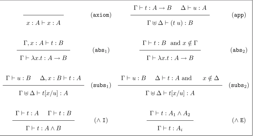
Definition 2.1 (category). A category C consists of objects obj(C) and arrows arr(C). Each arrowf is associated with a pair of objects dom(f)andcod(f)respectively called the domain and codomainoff. The notationf :A→Bindicates thatA(resp. B) is the domain (resp. codomain) off. For each objectA ofC, there is an arrowidA called the identity arrow.
The operation ◦ is called composition. If f : A →B and g : B → C then we can form the compositeg◦f :A→C which we sometimes abbreviate togf.
Cis required to satisfy the laws of associativity (h◦(g◦f) = (h◦g)◦f whencod(f) = dom(g)
andcod(g) = dom(h)) and unit ((f◦idA=f = idB◦f whenf :A→B).
Categories are quite like directed graphs in structure.1
Definition 2.2 (precategory). A precategory´C is defined exactly as a category, except that the composition of arrows is not always defined. Composition with the identities is always defined and the unit law always holds. The associativity law holds when the compositions are defined.
Definition 2.3(functor). A functor F :C→D between (pre)categories C and D is a mapping from objects of C to objects of D and arrows of C to arrows of D which satisfies the following laws:
• dom(F(f)) =F(dom(f))andcod(F(f)) =F(cod(f)),
• F(g◦f) =F(f)◦ F(g),
• F(idA) = idF(A).
1
2.2. CATEGORY THEORY CHAPTER 2. CONCEPTS AND TERMINOLOGY
These can be represented by the commuting diagrams below.
A f
F
B g
F
C
F
A idA
F
A
F
F(A) F(f) F(B) F(g) F(C) F(A) idF(A)F(A).
A functor may be informally thought of as a graph homomorphism.
Definition 2.4(homset). The set of arrows fromAtoB in a (pre)categoryCis called a homset and is denoted asHomC(A, B)orC(A→B).
Definition 2.5 (faithful, full functor). A functor F : C → D is faithful iff it is injective on homsets i.e. for all A, B∈obj(C), the mapping HomC(A, B)→HomD(F(A),F(B))is injective. A functorF:C→D is full iff it is surjective on homsets.
Definition 2.6 (subcategory). A functor F :C →D is a sub(pre)category when it is injective on objects and homsets. F defines a full subcategoryexactly when it is a full functor.
F is called an inclusion functor ofC in Dand is faithful by definition. Informally, we can think of subcategories similarly to subgraphs.
Definition 2.7 (tensor product, monoidal precategory). A(strict, symmetric) monoidal precate-gory has a partial tensor product⊗ both on objects and on arrows. It has a unit object ǫ, called the origin, such that I⊗ǫ=ǫ⊗I =I for all I. Given I⊗J andJ ⊗I it also has a symmetry isomorphismγI,J :I⊗J →J⊗I. The tensor and symmetries satisfy the following equations when both sides exist:
(1) f⊗(g⊗h) = (f⊗g)⊗handidǫ⊗f =f
(2) (f1⊗g1)(f0⊗g0) = (f1f0)⊗(g1g0)
(3) γI,ǫ= idI
(4) γJ,I◦γI,J = idI⊗J
2.2. CATEGORY THEORY CHAPTER 2. CONCEPTS AND TERMINOLOGY
Definition 2.8(s-category). An s-category´Cis a strict symmetric monoidal precategory which has:
• for each arrow f, a finite set |f| called its support, such that |idI| = ∅. For f : I → J and g : J →K the composition gf is defined iff |g| ∩ |f| =∅ and dom(g) = cod(f); then
|gf|=|g| ⊎ |f|. Similarly, forf :H →I andg:J →K withH⊗J andI⊗K defined, the tensor productf ⊗g is defined iff|f| ∩ |g|=∅; then|f⊗g|=|f| ⊎ |g|.
• for any arrow f : I → J and any injective map ρ whose domain includes |f|, an arrow ρ f :I→J called a support translation off such that:
(1) ρ idI = idI (5) (ρ1◦ρ0) f =ρ1 (ρ0 f)
(2) ρ (gf) = (ρ g)(ρ f) (6) ρ f = (ρ↾|f|) f
(3) ρ (f⊗g) =ρ f⊗ρ g (7) |ρ f|=ρ(|f|).
(4) Id|f| f =f
Each equation is required to hold only when both sides are defined.
Definition 2.9 (reflecting, preserving properties). A functor F : C → D is said to preserve a property if, given a collection of arrows and objects of C satisfying the property, the image in D
underF of that collection also has the property.
A functorF : C→D is said to reflect a property if, given a collection of arrows and objects ofC, if its image in Dunder F satisfies the property then so does the collection in C.
Definition 2.10 (support equivalence, supported functor). Two arrows f, g : I → J in an s-category ´Aare support-equivalent, written f ≏g, if ρ f =g for some support translationρ. By Definition 2.8 this is an equivalence relation. If ´Bis another s-category, then a supported functor
F : ´A →´B is a function on objects and arrows that preserves identities, composition, tensor product and support equivalence. IfF is an inclusion function then ´Ais a sub-s-categoryof ´B.
Notation. S-categories will be accented e.g.´C whereas categories are denoted asC. For conve-nience, we will write ‘subcategory’ for a subprecategory of an s-category.
2.2. CATEGORY THEORY CHAPTER 2. CONCEPTS AND TERMINOLOGY
Definition 2.12 (quotient categories). Let ´C be an s-category, and let ≡ be a congruence on ´C that includes support equivalence, i.e. ≏⊆ ≡. Then the quotient of ´C by ≡ is a category
Cdef=´C/≡, whose objects are the objects of ´Cand whose arrows are equivalence classes of arrows in ´C:
C(I, J)def
={[f]≡|f ∈´C(I, J)}.
InC, the identities, composition and tensor product are given by
idm
def
= [idm]≡
[g]≡◦[f]≡
def
= [gf]≡
[f]≡⊗[g]≡
def
= [f ⊗g]≡
By assigning empty support to every arrow, C may also be regarded as an s-category and [[·]]≡ : ´C→C is called the≡-quotient functorfor ´C.
In the following definition,Ordis the s-category of finite ordinals and functions between them.
Definition 2.13(wide s-category). An s-category ´A is wideif equipped with a functor width :
´A→Ordwith width(ǫ) = 0 such that, for each bijection πon the ordinal width(I), there is an isomorphismπI :I→I in ´Awith width(πI) =π.2
The objectsH, I, J, . . .of ´Aare calledinterfaces, and its arrowsA, B, C, . . .are called contexts. The domain and codomain of a context will be called its innerandouter faces. Arrows in a homset ´A(ǫ → I) – which is often abbreviated to ´A(I) – are called ground arrows; lower case letters a, b, . . .range over these, anda:ǫ→I can be abbreviated toa:I.
Definition 2.14 (span, cospan). A span is a pair of arrows with the same domain. Acospan is a pair of arrow with the same codomain.
~
f will be used to denote a span or a cospan of two arrows f0 and f1. It will be made clear whether the pair is a span or cospan. We writefi to denote one of f~andf¯ı to denote the other.
Definition 2.15 (bound, consistent). Given a span f~ : H → I~ and a cospan ~g : I~ → K, if g0f0 = g1f1, then it is said that ~g is a bound for f~. If f~ has any bound, then it is said to be consistent.
Bigraphs are arrows of specific categories. Composition in those categories is analogous to the placing of aλ-calculus term inside aλ-context. Bigraphs can also react, or reconfigure themselves,
2
In place-sorted bigraphs, the isomorphismsπI generally have domainIand codomainI′whereI6=I′. This is
2.2. CATEGORY THEORY CHAPTER 2. CONCEPTS AND TERMINOLOGY K I0 g0 h0 h I1 g1 h1 H
f0 f1
K k I0 g0 k0 h0 j h I1 g1 h1 k1 H
f0 f1
Figure 2.1: A relative bound(~h, h)forf~relative to~g (left) and a relative pushout (right)
according to reaction rules. This leads to a definition of labelled transition systems of bigraphs based on contexts. For example, ifaplaced in contextF can reconfigure toa′, we can writea F
_a′.
However, we would not wish to takeall contexts as labels as this would yield an intractably large relation over which to prove e.g. bisimilarity. Furthermore, Sewell points out that the induced behavioural equivalences are not satisfactory [140].
We want labels be to minimal in some sense – but in what exact sense? Leifer’s proposal [90] was to use the notion ofrelative pushout(RPO) to define minimal labels.
Definition 2.16 (relative pushout (RPO)). Let ~g:I~→K be a bound for f~:H →~I. Abound forf~relative to~g is a triple(~h, h)of arrows such that~his a bound for f~and hhi=gi(i= 0,1). The triple may be called a relative boundwhen~g is understood.
Arelative pushout (RPO) for f~relative to~gis a relative bound (~h, h)such that for any other relative bound(~k, k)there is a unique arrow j for whichjhi=ki(i= 0,1) andkj =h.
Specific RPOs are used as the labels of the labelled transition systems of bigraphical systems.3
Definition 2.17(idem pushout (IPO)). A pair~h:~I→J is an idem pushout (IPO)for the pair ~
f :H →~I if the triple(~h,idJ)is an RPO forf~to~h.
Definition 2.18 (pushout). A bound~g :I~→ J forf~ :H → ~I is a pushout forf~ if given any other bound~h:I~→K forf~, there exists a unique mediator j:J →K such that j◦gi=hi.
RPOs are pushouts in a slice category [90]. Specifically, the pushout (h0, h1, h) of a bound g0, g1with codomainKfor a pairf0, f1is a pushout in the slice category overK. This is depicted
3
2.2. CATEGORY THEORY CHAPTER 2. CONCEPTS AND TERMINOLOGY
E
D j
B d0 e0
C d1
e1
A c0 c1
K k I0 g0 k0 h0 j h I1 g1 h1 k1 H
f0 f1
k
h j
g0 h0 k0
g1 h1
k1
f0g0 f0 f1
(a) (b) (c)
Figure 2.2: (a)A pushout(d0, d1) of(c0, c1) inC (b) A relative pushout(~h, h) forf~relative to ~g inC (c)The same relative pushout as a pushout in the slice categoryC↓K
in Figure 2.2. Pushouts describe bounds which are least in some sense.4 An RPO is a triple
(h0, h1, h)such thath0 andh1 are minimal; this will hopefully become clearer once bigraphs are introduced. The intuition is thath0 andh1are the minimal contexts such thath0◦f0=h1◦f1; h0 (resp. h1) adds the least amount to f0 (resp. f1) such that their composition equals h1◦f1 (resp. h0◦f0). This intuition is invaluable when trying to find proofs of RPO creation for sorted bigraphs.
The notion of relative pushout is an example of a universal construction. We do not need to present the definition of universal construction here but it is a powerful concept.
Bigraphs benefit greatly from their categorical presentation. We will investigate sorted bigraphs in the following chapters. Sorted bigraphs form their own s-categories but they are linked to pure bigraphs viasorting functors which are forgetful and faithful. In well-behaved sortings, much of the pure theory can be reflected along this functor.
Definition 2.19(sorting functor). Asorting functoris surjective on objects and faithful. We adopt the terminology below for opfibrations from Jacobs and Birkedal et al. [72, 17]. Arrows or cospans with particular properties along sortings are instrumental to our proofs or RPO creation and pushout reflection. Jensen has presented conditions which are sufficient to prove that a sorting creates RPOs [73] whilst Leifer and Milner identified that if every arrow in an s-category is opcartesian with respect to a sorting functorU, then this is sufficient to prove pushout
4
2.2. CATEGORY THEORY CHAPTER 2. CONCEPTS AND TERMINOLOGY
reflection alongU [92].
Definition 2.20(above, vertical, lift at an object). LetF :´E→´Bbe a functor.
We say that an arrow f is above F(f). If f : I → J is above an identity then we call it a verticaland denote f by J↑I5.
Let E be an object of ´E. An arrow of ´B has a lift at E iff it is the F-image of an arrow f :E→X.
Definition 2.21 (opcartesian). An arrowf of a precategory ´Dis opcartesian with respect to a functorF:´D→´Ciff for allhwhereF(h) =g′◦ F(f), there exists a unique arrowg in ´Dsuch thatF(g) =g′ andh=g◦f.
g
. g′
_
Ff h
F(f)
F(h)
Definition 2.22 (weak opfibration). A functorF :´E→´B is a weak opfibration iff whenever an arrowf of ´B has a lift atE, it has an opcartesian lift atE.
The requirement that all arrows are opcartesian is quite strong. Birkedal, Debois, and Hilde-brandt consider the notion of jointly opcartesian cospan [17].
Definition 2.23(jointly opcartesian cospan). A cospan~gof a precategory´Disjointly opcartesian with respect to a functor F :´D →´C iff whenever ~his a cospan, g0, h0 is a span, and g1, h1 is a span in ´D with F(hi) = k′◦ F(gi), then there is a unique k in ´C such that hi =k◦gi and
F(k) =k′.
k k′
g0
h0
g1
h1
F(g0)
F(h0)
F(g1)
F(h1)
Definition 2.24(jointly opcartesian bound (JOB)). If a jointly opcartesian cospan~g is a bound forf~, we say that it is a jointly opcartesian bound (JOB) forf~.
5
2.3. PURE BIGRAPHS CHAPTER 2. CONCEPTS AND TERMINOLOGY
J J
I J↑I
I J↑I
H f
f′
H0 f0
f′ 0
H1 f1
f′ 1
Figure 2.3: A nearly opcartesian arrowf (left) and a nearly jointly opcartesian cospanf~(right)
If all arrows along a functor are opcartesian then all cospans along the functor are jointly opcartesian. We will work with cospans so the property of jointly opcartesian is weaker, more generally applicable, and just as sufficient. In Chapter 5, we consider a slightly weaker property.
Definition 2.25 (nearly opcartesian). An arrowf :H →J of ´E is nearly opcartesian if there exists a verticalJ↑I and an opcartesianf′ :H →I such thatf =J↑I◦f′.
Definition 2.26 (nearly jointly opcartesian). A cospan f~ : H~ → J of ´E is nearly jointly op-cartesian if there exists a vertical J↑Iˆ and a jointly opcartesian cospan f~′ : H~ → I such that fi=J↑Iˆ◦fi′, i∈ {0,1}.
2.3
Pure bigraphs
As described in the introduction, bigraphs are a framework for mobile computation and commu-nication which aims to both allow the modelling of ubiquitous computation and present a unified framework in which to analyse the behavioural equivalences of process calculi. In this section, we present some of the basic notions. The theory is quite detailed and we refer the reader to Jensen and Milner’s work [74, 114] for a detailed explanation.
We adopt Milner’s definitions and terminology for pure bigraphs which have been developed from work by Jensen and Milner [74, 113]. Informally, a pure bigraph is a combination of two graphs, the first of which is a partially ordered6 forest of trees called a place graph whilst the second is a hypergraph7called alink graph. The place graph models hierarchies of locations. This can be used to model containmente.g. the intruder is in the building, the PC is inside the firewall, theλ-variable is under theλ-abstraction. The link graph instead models connectivity, connecting
6
The set of roots is totally ordered, there is no order amongst children of a node.
7
2.3. PURE BIGRAPHS CHAPTER 2. CONCEPTS AND TERMINOLOGY
entities in a system to each other or to identifierse.g. the intruder is communicating with a foreign agent, the PC is linked to a WAN server, theλ-variable is namedx. These two graphs are largely independent, the intuition being “where you are doesn’t affect who you may talk to” [109]. For example, the foreign agent or the server may be located far from the intruder or PC respectively.
A category of bigraphs is defined over a signature. The signature specifies the entities of the system, called controls. In the informal intruder example above, the controls would include intruder, building, and foreign agent. The signature also specifies whether a control may contain other controls and the number ofports it has to link with other controls and names.
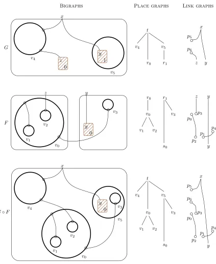
Figure 2.4 depicts three bigraphsG,F, andG◦F and their constituent place graphs and link graphs. A place graph is an ordered forest of trees. The nodes at the top of the trees (t in G, r0 andr1 inF) are special nodes calledroots. Some of the leaves are also special and are called sites e.g. r0 andr1in Gands0in F. These special nodes describe the interfaces of bigraphs, allowing us to compose two place graphs to form a larger one. In composition, one place graph is ‘planted’ inside the other by placing its roots inside the sites of the other. A link graph also involves nodes but it only cares about their ports (p0, . . . , p6 in the diagram). The ports are linked to each other and toinner andouter names. The names of a link graph allow us to compose two link graphs to form a larger one by ‘fusing’ the links together.
A bigraph is a combination of a link graph and a place graph with the same set of nodes. This shared setv0, . . . , v5 is the only overlap in the structures which are otherwise independent. The place graph is represented by a nesting of nodes, roots are represented by outer rectangles called regions, and sites are represented by shadedholes. The inner names of the link graph are placed at the bottom of the bigraph whereas the outer names sit up top. The bigraphGwith two sites and inner namesy andzmay be composed with a bigraph with two roots and outer namesyand z. The compositionG◦F plants F inside G, fuses the links, and forgets the places and names at the shared interface.
2.3. PURE BIGRAPHS CHAPTER 2. CONCEPTS AND TERMINOLOGY
000
000
000
000
111
111
111
111
00
00
00
00
11
11
11
11
000
000
000
111
111
111
00
00
00
11
11
11
z y x p5 p6 y y p0 p2 z p3 p4 p1 r0 v1 v0 v2 r1 s0 v3 v5 r1 r0 t v4 x p5 p6 p0 p2 p3 p4 p1 y v1 v2 v0 0 y y z v3 t v4 v5 v1 v0 v2 v3 s0 x v5 0 z 1 y 0 y x v4 v1 v2 v0 v3 v5 G v4 FG◦F
[image:43.595.104.527.121.638.2]Bigraphs Place graphs Link graphs
Figure 2.4: Bigraphs, place graphs, link graphs, and composition
2.3. PURE BIGRAPHS CHAPTER 2. CONCEPTS AND TERMINOLOGY 00 00 00 11 11 11 00 00 00 11 11 11 0 y x v4 v1 v2 v0 v3 v5 v2 0 y x v4 v1 v0 v3 v5
Figure 2.5: A bigraph reacts
of functions [88], the internal diagrams of bigraphs depicted in the figures are very informative themselves and we usually present them instead of formal terms.
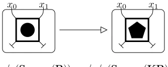
Bigraphs are not just static structures; they are a framework for modelling mobile computation. An s-category of bigraphs can be equipped with a set ofreaction rules. These reaction rules generate a reaction relation which describes how the bigraphs may reconfigure themselves. The s-category and its reaction rules together describe a bigraphical reactive system (Brs).8 The reaction rules may be parametric, meaning that only part of the redex and reactum is specified in the rule and that an actual redex is formed only when the parameters are supplied. This is a familiar notion; consider the substitution generation rule(λx.t)u→bt[x/u]of many explicit substitution calculi. The parameters here are the subtermstandu. Certain controls may prohibit reaction below them e.g. a guarded term of a process calculus. This is specified in the signature. Figure 2.5 depicts a reaction where the location ofv2has changed while its link withv4 is preserved andv4has lost its connection with the namex.
Our presentation of dynamic signature below differs (i.e. it has an explicitkind function) but is equivalent to the standard definition. We chose this presentation as it better highlights the changes we consider in the following chapters.
Definition 2.27(dynamic signature). Adynamic signatureK {K, arity, actv, kind} is composed of a setK of controls and three maps:
arity:K →N actv:K → {passive,active} kind:K → {∅,K}.
For each controlK,arity provides a natural number ar(K), an arity(the number of ports of the 8
2.3. PURE BIGRAPHS CHAPTER 2. CONCEPTS AND TERMINOLOGY
control). Theactv function determines which controls allow reaction inside them (activecontrols) and which do not (passivecontrols). Ifkind(K) =K thenK may contain other controls or sites and is called non-atomic. Otherwise, it may not contain any control or site in a bigraph and is termed atomic.
Atomic controls cannot contain other controls and so, along with passive controls, do not allow reaction inside them; active controls do.
Finally, the operational semantics of a Brs is given by the reaction relation and a labelled transition system (LTS). This is where the general framework becomes quite powerful. There is a standard notion of label (as context) for Brss based on RPOs and hence canonical labelled transition systems. This avoids the need to manually (ad hoc) derive an LTS. The LTSs of the encodings of the calculi mentioned in the introduction correspond closely to the original calculi. We discuss labels in more detail in Chapter 5.
Notation. WhenA~ denotes a pair of arrowsA0 andA1, we let irange over{0,1},¯ı=