Contents lists available atScienceDirect
Global Ecology and Conservation
journal homepage:www.elsevier.com/locate/gecco
Original research article
Factors influencing when species are first named and
estimating global species richness
Mark J. Costello
a,∗, Marguerita Lane
a,b, Simon Wilson
b, Brett Houlding
baInstitute of Marine Science, University of Auckland, Auckland 1142, New Zealand bDiscipline of Statistics, Trinity College Dublin, Ireland
a r t i c l e i n f o
Article history:
Received 23 April 2015
Received in revised form 5 July 2015 Accepted 5 July 2015
Available online 24 July 2015
Keywords:
Biodiversity Biogeography Marine Freshwater Fish Taxonomy
a b s t r a c t
Estimates of global species richness should consider what factors influence the rate of species discovery at global scales. However, past studies only considered regional scales and/or samples representing<0.4% of all named species. Here, we analysed trends in the rate of description for all fish species (2% of all named species). We found that the number of species described has slowed for (a) brackish compared to marine and freshwater species, (b) large compared to small sized fish, (c) geographically widespread compared to localised, (d) species occurring in the tropics and northern hemisphere compared to southern hemi-sphere, and (e) neritic (coastal) species compared to pelagic (offshore) species. Most (68%) of the variation in year of description was related to geographic location and depth, and contrary to expectations, body size was a minor factor at just 6% (on a standardised scale). Thus most undiscovered species will have small geographic ranges, but will not necessarily be of smaller body size than currently known species. Accordingly, global assessments of how many species may exist on Earth need to account for geographic variation.
©2015 The Authors. Published by Elsevier B.V. This is an open access article under the CC BY license (http://creativecommons.org/licenses/by/4.0/).
1. Introduction
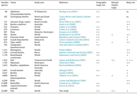
Knowing how many species are on Earth is amongst the most topical questions in biology and ecology, because it defines progress in the rate of discovery of life. However, the discovery of species is not random. The system of describing species initiated by Linnaeus began in Europe in the 1750’s and spread around the world as Europeans travelled and/or had material collected from other parts of the world and brought to them for description. Knowing where new species are most likely to be found enables targeted expeditions (e.g.Brandt et al., 2007,Bouchet,2009;Bouchet et al.,2009) and helps justify research funding applications. However, studies looking at factors influencing the rate of species discovery have been limited in spatial extent, taxonomic coverage, number of species and variables examined (Table 1).
Global scale analyses considered body size for passerine birds (Gaston and Blackburn, 1994), monogenean trematodes and crustaceans (Poulin,2002;Martin and Davis, 2006), and body size and geographic range for terrestrial Carnivora and Primates (Collen et al., 2004) and branchiopod crustaceans (Adamowicz and Purvis, 2005). In addition to these two factors, depth distribution was studied for marine holozooplankton (species planktonic for all of their life-cycle) (Gibbons et al., 2005). However, the variables examined varied between studies and some results were contradictory. For example, half the studies found body size was a poor or insignificant predictor of year of description (Table 1). A more global perspective of a wide range of variables for a species rich taxon would provide a more accurate assessment of what factors most influence
∗Corresponding author.
E-mail address:m.costello@auckland.ac.nz(M.J. Costello).
http://dx.doi.org/10.1016/j.gecco.2015.07.001
Table 1
A review of factors correlated with the rate of discovery in different taxa in the literature. The strength of correlations is indicated as++strong,+weak but positive, ns=not significant.
Number species
Taxon Study area Reference Geographic
range size
Altitude (depth) range
Body size
84 Aphthoma
Chrysomelidae beetles
W Palaearctic Baselga et al.(2007) ++ ns 102 Geotrupinae beetles North and South
America
Trotta-Moreu and Cabrero-Sañudo
(2010)
++ ns
131 Anurans (frogs, toads) Brazil Cerrado Diniz-Filho et al.(2005) ++ ++
156 Beetles rainforest Australia Stork et al.(2008) ++
232 Primates World Collen et al.(2004) ++ +
270 Carnivora World Collen et al.(2004) ++ ++
297 Fleas Holarctic, Neotropics Krasnov et al.(2005) ++
493 Sharks World Randhawa et al.(2014) ++ + ++
539 Passerine birds South America Blackburn and Gaston(1995) ++ +
629 Scarab dung beetles Palaearctic Cabrero-Sañudo and Lobo(2003) ++ +
672 Tiger moths Brazil Ferro and Diniz(2008) + + ++
792 Tardigrades limnoterrestrial
World Guil and Cabrero-Sanudo(2007) ++
1,131 Monogenea World Poulin(2002) ++
1,158 Ground beetles Iberia Jiménez-Valverde and Ortuño(2007) ++ ++
1,176 Branchiopod crustaceans
World Adamowicz and Purvis(2005) ++ +
1,222 Fish Tropical east Pacific Zapata and Robertson(2007) ++ ++ + + +
1,145 Mammals Neotropics Patterson(1994) ++ ++
1,433 Reptiles, amphibians North America, Australia
Reed and Boback(2002) +
3,441 Scarab beetles Australia Allsopp(1997) ++ +
3,637 Beetles Britain Gaston(1991b) +
4,000 Marine holozooplankton
World Gibbons et al.(2005) ++ + +
6,209 Birds World Gaston and Blackburn(1994) ++
21,000 Butterflies North American Gaston et al. (1995a,b) ++ ++
24,092 Land & freshwater animals
Europe Essl et al.(2013) ++
32,000 Fish World This study ++ ++ +
when and where species will be discovered than previous studies. Because fish are the most diverse group of vertebrates and present throughout the world’s oceans and freshwater environments, we suggest they may be representative of the factors that will influence the rate of discovery of other species on Earth. Fish provide a wider combination of species richness, body size, environmental and global coverage (freshwater and marine), than previous studies, represent ca. 2% of all named species (Costello et al.,2013a,b), and thus may better reflect global taxonomic trends.
Here, we have compared the rates of description of all fish with their geographic location, body size, environment, and number of species in a genus (i.e. number of congeners) (Table 2). We expected that species would tend to have been discovered sooner if they were (a) more conspicuous due to their larger body size, (b) more encountered if they had a greater geographic and depth range, and occurred in high latitudes (e.g. Europe, North America), and (c) easier to distinguish if there were fewer species in the genus (differences between genera will generally be more obvious than differences between species). The results show the importance of including biogeographic patterns in estimating global species richness.
2. Methods
We compiled data on the year of description, geographic and environmental distribution, habitat, and maximum body size for all fish species from FishBase on 10th June 2011 (Froese and Pauly, 2014). This data is available in the online Supplementary Material (seeAppendix A).Reuman et al.(2014) found these data were representative of animal body mass from 1 to 1,000 kg and that maximum length was a reasonable indicator of asymptotic length. Not all of the variables were available for all 32,055 species, so sample size varied (Table 3). A species geographic range was estimated by (a) the distance between its northern- and southern-most latitude, and eastern and western-most longitude, (b) the number of Food and Agriculture Organisation (FAO) fishery management areas the species was present in, and (c) the number of countries it was present in. There were 15,779 only freshwater, 1,496 only brackish, and 16,953 only marine species.
The following equations were used to predict range from the limits of a species latitude and longitude observations. If the species’ longitudinal range was 360°, then geographic area (in km2) was calculated as:
Table 2
The potential relationship of the variables analysed in this study to the year of species description. Variable Species that are more likely to be discovered earlier
Geographic range
Species range area
Species with a wider geographic range. Countries present
FAO areas present Latitude range Longitude range
Geographic location
Latitude northern
Species located near more developed countries, particularly Europe where the taxonomic system originated.
Latitude southern Latitude mean Longitude western Longitude eastern Longitude mean
Depth
Minimum depth
Species occurring in shallower depths. Depth range
Number spp in genus Species so different from named species that they form the basis for a new genus.
[image:3.544.38.504.312.600.2]Maximum length Larger species.
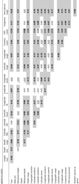
Table 3
Coefficients for the variables for the Principal Components (PC) Analysis that together described 96% of the variation. Values>0.3 are shaded.N =
number of fish with variable. Note that data with missing values was handled by generating a correlation matrix using R’s ‘‘pairwise.complete.obs’’ option in the cor() function, so that the correlation between each pair of variables is computed using all complete pairs of observations on those variables.
Variables N PC1 PC2 PC3 PC4 PC5 PC6 PC7 PC8 PC9 PC10
Geographic range
Species range area 3,041 −0.37 −0.09 0.04 0.03 0.19 −0.20 −0.28 0.04 0.15 0.41 Countries present 31,228 −0.36 0.01 0.14 −0.23 0.07 0.12 −0.01 −0.22 0.06 −0.16 FAO areas present 31,995 −0.40 −0.05 0.11 0.04 0.09 −0.05 0.13 −0.06 0.03 −0.26 Latitude range 8,942 −0.41 −0.03 0.08 −0.05 0.08 −0.18 −0.16 −0.08 −0.01 0.26 Longitude range 3,042 −0.33 −0.15 −0.09 0.23 0.11 0.00 0.29 −0.15 0.22 −0.57
Geographic location
Latitude northern 9,300 −0.21 0.50 0.10 0.09 0.09 −0.12 −0.08 −0.10 0.11 0.13 Latitude southern 9,070 0.19 0.53 0.03 0.13 0.02 0.05 0.07 −0.02 0.12 −0.16 Latitude mean 8,942 −0.01 0.59 0.08 0.12 0.06 −0.03 −0.01 −0.06 0.12 −0.03 Longitude western 3,057 0.23 −0.12 0.37 −0.05 0.21 −0.33 −0.38 0.31 0.30 −0.33 Longitude eastern 3,046 0.03 −0.08 0.56 0.26 −0.05 0.23 0.31 −0.27 −0.20 0.25 Longitude mean 3,042 0.16 −0.13 0.62 0.15 0.09 −0.04 0.00 −0.02 0.04 −0.02
Depth
Minimum depth 11,760 0.01 −0.09 −0.15 0.59 −0.02 0.32 −0.64 −0.26 −0.10 −0.12 Depth range 11,159 −0.17 0.00 −0.08 0.57 0.00 −0.21 0.25 0.61 −0.21 0.07
Number spp in genus 32,055 0.08 0.01 −0.10 −0.07 0.88 0.39 0.08 0.14 −0.12 0.07 Maximum length 27,943 −0.21 0.02 0.14 −0.08 −0.28 0.65 −0.05 0.46 0.45 0.08 Year 32,055 0.22 −0.19 −0.22 0.26 0.11 −0.11 0.25 −0.25 0.69 0.30
Variance 4.76 2.75 2.08 1.29 0.99 0.91 0.78 0.73 0.63 0.41 Proportion of variance 0.30 0.17 0.13 0.08 0.06 0.06 0.05 0.05 0.04 0.03
Cumulative proportion of variance explained 0.30 0.47 0.60 0.68 0.74 0.80 0.85 0.89 0.93 0.96
where 6378.127 is the radius of the Earth in kilometres and
|
x|
means the absolute value ofx. Otherwise, geographic area was calculated as:2
π
∗
6378.
1272∗|
sin(
Lat N.)
−
sin(
Lat S.)
| ∗
Longitude Range.
measured by their mutual co-variation. Regression coefficients identified if the variable significantly influenced whether a species was described earlier or later. Finally, the step AIC function was used in the open source statistical programme R (R Core Team, 2011) to add and remove variables until the model could no longer be improved in terms of lowering the Akaike Information Criterion (AIC) through further iterations (Burnham and Anderson, 2002).
To predict how many more species may be discovered from the past rate of descriptions, we applied theWilson and Costello(2005) Non-Homogeneous Renewal Process (NHRP) model based on extrapolation of the discovery curve as a logistic function with the form:
Number discovered by yeart
=
N 1+exp(−β(t−α)).This takes on an ‘S’ shape, going from 0 att
= −∞
toNatt= +∞
. The logistic function is a popular choice as a model for the trend in species discovery in a taxon, as it has the property of an initial slow rate of discovery, rising to a peak before discoveries tail off when most of the species in the taxon are described. The three parameters of the function were:N, the total number of species to be discovered;α
, the year of maximum rate of discovery; andβ
which describes the overall rate of discovery, with a largerβ
implying a faster rate. This model is stochastic and describes the time between discoveries of species as a renewal process where the mean number discovered as a function of time follows a logistic function. Bayesian statistical inference methods were used to fit the discovery curve to this model, giving an estimate of the three parameters of the logistic function and in particular an estimate ofN, the total number of species. This produced an estimate of the number of species in the taxon remaining to be described. Predictions based on extrapolating a logistic curve are very sensitive to the fitted value ofα
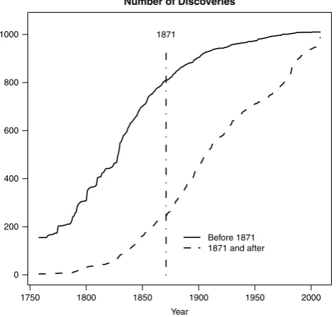
, the date of maximum rate of discovery. Our methodology was to use the information on species traits and location to predict when a species should have been described. We then split the data into two cohorts, namely those with an early predicted year of description, and those with a later year of description, and applied the aforementioned NHRP independently on these two cohorts. We found the median predicted discovery year for the 1,997 ‘best-documented’ species for which all the significant predictor variables (asterisked inTable 5) were available was in the year 1871, whilst it was 1932 for all 32,055 species recorded in FishBase. This was because the more recently discovered species were less likely to have all the significant predictor variables recorded due to lack of time for their study. We divided the 1,997 species with all recorded predictor variables, into a group of 1,010 species whose predicted discovery time, based on their location and other attributes, was before the median discovery year of 1871, and 987 whose predicted time was after 1871. Then the NHRP model was run on the two groups separately, using the real discovery year of the species in the two groups as the data, so as to examine the effect on predicting the total number of species based on only considering species with geographic ranges and locations etc. suggesting early discovery, and those whose geographic ranges and locations etc. suggested later discovery.3. Results
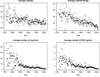
Almost all of the variables considered were significantly correlated with year of discovery (Table 4). However, their relative contribution varied (Tables 5and6). Thus the number of species described has slowed for (a) brackish compared to marine and freshwater species, (b) large compared to small sized fish, (c) geographically widespread compared to localised, (d) species occurring in the tropics and northern hemisphere compared to southern hemisphere, and (e) neritic (coastal) species compared to pelagic offshore species (Fig. 1). Fish continued to be discovered from all depths in the oceans, but deep sea fish only began to be discovered from the 1890’s (Fig. 2). Species with wider geographic ranges and occurring in more northerly latitudes and closer to the Greenwich meridian of longitude have been described earlier (Fig. 3). Regression analysis also supported the link between wider geographic range (in terms of latitude and the number of countries in which the species was found) and earlier year of discovery (Table 5). Controlling for other factors, brackish and freshwater species were likely to be discovered on average 25 years and 11 years earlier, respectively, than a marine species (Table 5). The rate of description of small fish had overtaken that of medium and large fish since the 1960’s, although new species continued to be described of all body sizes (Fig. 4). Indeed, recent years have seen an unprecedented number of species described per year overall (Fig. 5), and especially of small fish (Fig. 4). Species in genera with few species have been discovered earlier, reflecting the greater morphological differences between genera than species (Fig. 6andTable 5).
The PCA identified which of the variables were most important in explaining the variation in the dataset (Table 2). As seen, 30% of variation in the data was accounted for by a single linear combination of the variables which focused on how widespread species were, and a further 30% by two linear combinations both of which focused on geographic location, particularly latitude (Table 2). Depth and depth range explained a further 8% of variation, and the number of species in the genus and body size a further 6%.
Table 5
Linear regression coefficients. The dependent variable was year of discovery (n=2020, multipleR2:0.4201). Positive values indicate the variable leads
to later discovery, and negative to earlier. Coefficients marked with an asterisk were statistically significant, exceeding the 95% confidence level.
Variable Estimate Standard error tvalue
Mean latitude,+ve numbers north of equator −0.725 0.052 −13.981 ***
Latitude range −0.617 0.068 −9.039 ***
No. countries in which species is found −0.824 0.079 −10.409 ***
Binary variable=1 if brackish −25.300 3.590 −7.064 ***
Binary variable=1 if reef-associated −29.400 4.960 −5.940 ***
Binary variable=1 if demersal −23.800 4.830 −4.930 ***
Binary variable=1 if Bathypelagic 26.400 5.600 4.712 ***
Minimum depth 0.016 0.005 3.379 ***
Longitude range 0.065 0.020 3.308 ***
Binary variable=1 if pelagic 51.800 17.000 3.039 **
No. species in genus 0.102 0.043 2.404 *
Binary variable=1 if pelagic–oceanic 14.900 7.220 2.060 *
Binary variable=1 if freshwater −11.000 5.380 −2.044 *
Depth range −0.004 0.002 −1.852
Binary variable=1 if pelagic–neritic −7.580 6.050 −1.251 No. FAO regions in which species is found −0.998 0.804 −1.241
Maximum body length −0.002 0.001 −1.138
Binary variable=1 if Bentho-pelagic −1.870 5.420 −0.346
(Intercept) 1940.00 5.010 386.193 ***
[image:6.544.42.508.336.383.2]*P<0.05. **P<0.01. ***P<0.001.
Table 6
The 95% confidence limits of the number of new species predicted to be discovered by the statistical model by 2050 and 2100 for marine and brackish combined, and freshwater environments.
Present species Predicted new species by 2050 Predicted new species by 2100
Marine and brackish 18,449 3800 4300 8,100 9,300
Freshwater 15,779 4100 4800 7,800 9,900
Total 34,228 7900 9100 15,900 19,200
The model predicted that 21%–23% more new marine and brackish (combined) species would be described by 2050, and 44%–50% by 2100 (Table 6). For freshwater species the predictions were 26%–30% and 49%–60% by 2050 and 2100 respectively. The uncertainty in these predictions was higher for freshwater than for non-freshwater species. In both cases a description rate of roughly 1000 species per decade was predicted throughout this century with no evidence yet that the rate of discovery is declining. However, the number of authors describing new species has been increasing faster than the rate of new species description since the 1950’s (Fig. 5). This suggests that the continued rate of discovery is being maintained by increasing effort.
4. Discussion
4.1. Geography
The first three Principal Components accounted for a cumulative 60% of the variation in the discovery records, and each of these focused on aspects of geographic range and location (Table 2). The fourth Principal Component on depth then explained a further 8%.Blackburn and Gaston(1995) also found it explained 60% of the variance in the rate of discovery of South American passerine birds, andGuil and Cabrero-Sanudo(2007) 40% for tardigrades. Of the 18 studies that looked at geographic range, 17 found it significant and/or a primary predictor (Table 1). Only for moths in Brazil was it a weaker correlate, reflecting the narrower geographic scope of that study. Only two studies in addition to ours looked at geographic location; both found it significant for Palaearctic scarab and chrysomelid beetles.Gibbons et al.(2005) suggested location was also important for zooplankton but did not analyse it quantitatively. Species with a wider depth or altitudinal range were described earlier for tropical east Pacific fish, world sharks, tiger moths and in the present study (Table 1).
Fig. 1. Cumulative proportions or numbers of species described per year: top left by water type (brackish=dotted line; saltwater=solid line; freshwater=dashed line); top right by maximum body length (dotted line>220 mm; dashed line 90–220 mm; solid line<90 mm); middle left by geographic range (solid line=1 FAO area; dashed line=2 or 3; dotted line=4 or more); middle right by demersal and reef (solid line), pelagic (dashed line), neritic (dotted line) and oceanic (dash–dot line) species; bottom left by geographic range size being small (solid line), to large (dotted line); and bottom right by mean latitude (solid line<−2°; mid-latitudes 2–13°; dotted line>13°). The latter two plots show actual numbers described.
4.2. Body size
Fig. 2. The cumulative rate of description of species by depth. Top left panel shows minimum depth in shallow (solid line,<3 m), to deep (dotted line,
>75 m) waters. Top right panel shows small (solid line<20 m), to large (dotted line>196 m) depth ranges. Dashed lines are fish in the intermediate categories. Lower left is the average minimum depth, and lower right the depth range, of the species described in a year. Species at greater minimum depth have been discovered later, but those at shallow depths also continue to be discovered.
[image:8.544.105.445.385.648.2]Fig. 4. The number of species described by body length size each year (solid line<90 mm; dashed line 90–220 mm; dotted line>220 mm), and the maximum length of species described each year (right panel).
Fig. 5. The number of fish species named (dashed line), and the number of authors (solid line) who named fish species, in 10 year intervals.
[image:9.544.154.387.493.671.2]Fig. 7. The actual rate of description for species predicted to be discovered before (solid line) and after (dashed line) 1871 based on their location and other attributes.
4.3. Other factors
We found only a weak effect of the number of species in a genus, as did studies on North American butterflies (Gaston et al., 1995a), and terrestrial Carnivora and Primates (Collen et al., 2004). It was not significant for Iberian ground beetles and tiger moths in Brazil (Table 1). In addition to the factors studied here, strong correlations with description rates were found for colour of tiger moths in Brazil, trophic generalist chrysomelid beetles, and non-specialist habitat in Iberian ground beetles (Table 1). The latter two generalist factors are related to how geographically widespread a species may be and thus likely to be sampled. In rainforests, canopy living and plant-feeding beetles were better described than ground living species (Stork et al., 2008). Sharks at higher trophic levels have been described earlier although this will be correlated with larger body size (Randhawa et al., 2014). More host-specific parasitic helminths of freshwater fish in Canada (Poulin and Mouillot, 2005) and fleas (Krasnov et al., 2005) have also been described later. In summary, species living in more localised geographic areas and specialised habitats tend to be discovered later. It must also be remembered that an as yet unknown proportion of the 32,000 currently accepted scientific names for fish will be found to be synonyms, thereby reducing the number of known species and estimates of those to be discovered (Costello, 2015).
4.4. Undiscovered species
Overall we predicted between about 4,000–10,000 new marine and new freshwater species (each) may be discovered this century. That is, by 2050 about 21%–23% more marine and 26%–30% more freshwater species will be named. However, about twice these percentages may be discovered by 2100. Other estimates of how many fish species remain to be discovered ranged from 2%–30%: namely 30% (i.e. 5,000 or 22%) of all marine fish (Eschmeyer et al.,2010;Costello et al.,2012); 12%–15% of tropical East Pacific fish (Zapata and Robertson, 2007); 2%–5% of freshwater fish in Europe (Essl et al., 2013); and 13% (2,300) of freshwater fish globally (Pelayo-Villamil et al., 2015).
New species are most likely to have small geographic ranges, occur in the southern hemisphere, at greater depth range and deeper minimum depth, and be of smaller body size (Figs. 1–4). Estimates of global species richness need to account for the facts that most species are known in the northern hemisphere and that most species occur in the tropics. Discoveries of many new species in previously little sampled and remote locations are to be expected. However, such discoveries fill geographic gaps rather than alter the global pattern of species richness and biogeography, as found for freshwater fish (Pelayo-Villamil et al., 2015). Combining knowledge on present biogeographic patterns of species richness with the factors influencing rates of species discovery can inform predictions of how many more species will be discovered. For example, the paucity of deep-sea species being discovered in recent decades is notable. This may be because it has fewer endemic species than shallow seas (Ekman, 1953), and so many species that occur there may already have been found in shallower depths. Thus the discoveries of new species in less explored locations will only alter global patterns of species richness if those locations prove to have a higher density of species than better explored areas. This will not be the case for the pelagic and deep-sea because species there have larger geographic and depth ranges due to these environments being more homogenous and generally lower in temperature, topography and productivity than coastal seas. The similar number of fish species in marine and freshwater environments, despite their greatly different area and productivity, suggests that dispersal barriers are the primary cause of high species richness at global scales (Levêque et al.,2008;Vega and Wiens, 2012).
The most species rich areas on land and sea are in the tropics. In the ocean, the Caribbean in the Atlantic and SE Asia in the Pacific have highest species richness (e.g. for fishLevêque et al.,2008;Allen,2014). In contrast, the southern hemisphere ocean is largely deep and pelagic with less coastal seas than in the northern hemisphere. We thus agree withEschmeyer et al.(2010) that most new species of marine fish would be found in deep-slope and tropical reef habitats. While our findings indicated that significant numbers of new species are predicted to occur in the southern hemisphere, it is doubtful that these will significantly change the overall pattern of global fish species richness.
Acknowledgements
We thank Nicolas Bailly (WorldFish) for providing the export of data from FishBase, and Xingli Giam for helpful comments that improved the paper.
Appendix A. Supplementary data
Supplementary material related to this article can be found online athttp://dx.doi.org/10.1016/j.gecco.2015.07.001.
References
Adamowicz, S.J., Purvis, A.,2005. How many branchiopod crustacean species are there? Quantifying the components of underestimation. Glob. Ecol. Biogeogr. 14, 455–468.
Allen, G.R.,2014. Review of Indo-Pacific coral reef fish systematics: 1980 to 2014. Ichthyol. Res. 1–7.
Allsopp, P.G.,1997. Probability of describing an Australian scarab beetle: influence of body size and distribution. J. Biogeogr. 24, 717–724.
Alroy, J.,2002. How many named species are valid? Proc. Natl. Acad. Sci. USA 99, 3706–3711.
Appeltans, W., Ahyong, S.T., Anderson, G., Angel, M.V., Artois, T., Bailly, N., Bamber, R., Barber, A., Bartsch, I., Berta, A., Błazewicz-Paszkowycz, M., Bock, P., Boxshall, G., Boyko, C.B., Brandão, S.N., Bray, R.A., Bruce, N.L., Cairns, S.D., Chan, T.Y., Chan, L., Collins, A.G., Cribb, T., Curini-Galletti, M., Dahdouh-Guebas, F., Davie, P.J.F., Dawson, M.N., De Clerck, O., Decock, W., De Grave, S., de Voogd, N.J., Domning, D.P., Emig, C.C., Erséus, C., Eschmeyer, W., Fauchald, K., Fautin, D.G., Feist, S.W., Fransen, C.H.J.M., Furuya, H., Garcia-Alvarez, O., Gerken, S., Gibson, D., Gittenberger, A., Gofas, S., Gómez-Daglio, L., Gordon, D.P., Guiry, M.D., Hoeksema, B.W., Hopcroft, R., Jaume, D., Kirk, P., Koedam, N., Koenemann, S., Kolb, J.B., Kristensen, R.M., Kroh, A., Lambert, G., Lazarus, D.B., Lemaitre, R., Longshaw, M., Lowry, J., Macpherson, E., Madin, L.P., Mah, C., Mapstone, G., McLaughlin, P., Meland, K.L., Messing, C.G., Mills, C.E., Molodtsova, T.N., Mooi, R., Neuhaus, B., Ng, P.K.L., Nielsen, C., Norenburg, J., Opresko, D.M., Osawa, M., Paulay, G., Perrin, W., Pilger, J.F., Poore, G.C.B., Pugh, P., Read, G.B., Reimer, J.D., Rius, M., Rocha, R.M., Rosenberg, G., Saiz-Salinas, J.I., Scarabino, V., Schierwater, B., Schmidt-Rhaesa, A., Schnabel, K.E., Schotte, M., Schuchert, P., Schwabe, E., Segers, H., Self-Sullivan, C., Shenkar, N., Siegel, V., Sterrer, W., Stöhr, S., Swalla, B., Tasker, M.L., Thuesen, E.V., Timm, T., Todaro, A., Turon, X., Tyler, S., Uetz, P., van der Land, J., van Ofwegen, L.P., van Soest, R.W.M., Vanaverbeke, J., Vanhoorne, B., Walker-Smith, G., Walter, T.C., Warren, A., Williams, G., Wilson, S.P., Hernandez, F., Mees, J., Costello, M.J.,2012. The magnitude of global marine species diversity. Curr. Biol. 22, 1–14.
Baselga, A., Hortal, J., Jiménez-Valverde, A., Gómez, J.F., Lobo, J.M.,2007. Which leaf beetles have not yet been described? Determinants of the description of Western PalaearcticAphthonaspecies (Coleoptera: Chrysomelidae). Biodivers. Conserv. 16, 1409–1421.
Blackburn, T.M., Gaston, K.J.,1995. What determines the probability of discovering a species? A study of South American oscine passerine birds. J. Biogeogr. 22, 7–14.
Bouchet, P.,1997. Inventorying the molluscan diversity of the world: what is our rate of progress? Veliger 40, 1–11.
Bouchet, P.,2009. From specimens to data, and from seashells to molluscs: the Panglao Marine Biodiversity Project. Vita Malacol. 8, 1–8.
Bouchet, P., Lozouet, P., Sysoev, A.,2009. An inordinate fondness for turrids. Deep Sea Research Part II 56 (19), 1724–1731.
Brandt, A., Gooday, A.J., Brandao, S.N., Brix, S., Brökeland, W., Cedhagen, T., et al.,2007. First insights into the biodiversity and biogeography of the Southern Ocean deep sea. Nature 447 (7142), 307–311.
Brûlé, S., Touroult, J.,2014. Insects of French Guiana: a baseline for diversity and taxonomic effort. ZooKeys 434, 1–11.
Burnham, K.P., Anderson, D.R.,2002. Model Selection and Multimodel Inference: A Practical Information-Theoretic Approach, 2nd ed. Springer-Verlag, New York.
Cabrero-Sañudo, F.J., Lobo, J.M.,2003. Estimating the number of species not yet described and their characteristics: the case of Western Palaearctic dung beetle species (Coleoptera, Scarabaeoidea). Biodivers. Conserv. 12, 147–166.
Chevan, A., Sutherland, M.,1991. Hierarchical partitioning. Amer. Statist. 45, 90–96.
Collen, B., Purvis, A., Gittleman, J.L.,2004. Biological correlates of description date in carnivores and primates. Glob. Ecol. Biogeogr. 13, 459–467.
Costello, M.J.,2015. Biodiversity: the known, unknown and rates of extinction. Curr. Biol. 25 (9), R368–R371.
Costello, M.J., Emblow, C.S., Picton, B.E.,1996. Long term trends in the discovery of marine species new to science which occur in Britain and Ireland. J. Mar. Biol. Assoc. U. K. 76, 255–257.
Costello, M.J., Houlding, B., Joppa, L.,2014b. Further evidence of more taxonomists discovering new species, and that most species have been named: response to Bebber et al. 2014. New Phytol. 202, 739–740.
Costello, M.J., Houlding, B., Wilson, S.,2014a. As in other taxa, relatively fewer beetles are being described by an increasing number of authors: Response to Löbl and Leschen. Sys. Entomol. 39, 395–399.
Costello, M.J., May, R.M., Stork, N.E.,2013a. Can we name Earth’s species before they go extinct? Science 339, 413–416.
Costello, M.J., May, R.M., Stork, N.E.,2013b. Response to comments on can we name Earth’s species before they go extinct? Science 341, 237.
Costello, M.J., Vanhoorne, B., Appeltans, W.,2015. Conservation of biodiversity through taxonomy, data publication and collaborative infrastructures. Conserv. Biol. 29 (4), 1094–1099.
Costello, M.J., Wilson, S.P.,2011. Predicting the number of known and unknown species in European seas using rates of description. Glob. Ecol. Biogeogr. 20, 319–330.
Costello, M.J., Wilson, S.P., Houlding, B.,2012. Predicting total global species richness using rates of species description and estimates of taxonomic effort. Syst. Biol. 61 (5), 871–883.
Costello, M.J., Wilson, S., Houlding, B.,2013c. More taxonomists but a declining catch of species discovered per unit effort. Syst. Biol. 62 (4), 616–624.
Diniz-Filho, J.A.F., Bastos, R.P., Rangel, T.F.L.V.B., Bini, L.M., Carvalho, P., Silva, R.J.,2005. Macroecological correlates and spatial patterns of anurans description dates in Brazilian Cerrado. Glob. Ecol. Biogeogr. 14, 469–477.
Ekman, S.,1953. Zoogeography of the sea. Sidgwick & Jackson, London, p. 417.
Eschmeyer, W.N., Fricke, R., Fong, J.D., Polack, D.A.,2010. Marine fish diversity: history of knowledge and discovery (Pisces). Zootaxa 2525, 19–50.
Essl, F., Rabitsch, W., Dullinger, S., Moser, D., Milasowszky, N.,2013. How well do we know species richness in a well-known continent? Temporal patterns of endemic and widespread species descriptions in the European fauna. Glob. Ecol. Biogeogr. 22 (1), 29–39.
Ferro, V.G., Diniz, I.R.,2008. Biological attributes affect the data of description of tiger moths (Arctiidae) in the Brazilian Cerrado. Divers. Distrib. 14 (3), 472–482.
Fontaine, B., van Achterberg, K., Alonso-Zarazaga, M.A., Araujo, R., Asche, M., et al., 2012. New species in the Old World: Europe as a frontier in biodiversity exploration, a test bed for 21st century taxonomy. PLoS ONE 7 (5), e36881.http://dx.doi.org/10.1371/journal.pone.0036881.
Froese, R., Pauly, D. (Eds.), 2014. FishBase. World Wide Web Electronic Publication, version (08/2014)www.fishbase.org. Gaston, K.J.,1991b. Body size and probability of description: the beetle fauna of Britain. Ecol. Entomol. 16, 505–508.
Gaston, K.J., Blackburn, T.M.,1994. Are newly described bird species small-bodied? Biodivers. Lett. 2, 16–20.
Gaston, K.J., Blackburn, T.M., Loder, N.,1995a. Which species are described first? The case of North American butterflies. Biodivers. Conserv. 4, 119–127.
Gaston, K.J., Scoble, M.J., Crook, A.,1995b. Patterns in species description: a case study using the Geometridae (Lepidoptera). Biol. J. Linn. Soc. 55, 225–237.
Gibbons, M.J., Richardson, A.J., Angel, M.V., Buecher, E., Esnal, G., Fernandez-Almo, M.A., Gibson, R., Itoh, H., Pugh, P., Boettger-Schnack, R., Thuesen, E.,2005. What determines the likelihood of species discovery in marine holozooplankton: is size, range or depth important? Oikos 109, 567–576.
Guil, N., Cabrero-Sanudo, F.J.,2007. Analysis of the species description process for a little known invertebrate group: the limnoterrestrial tardigrades (Bilateria, Tardigrada). Biodivers. Conserv. 16 (4), 1063–1086.
Irfanullah, H.M.,2013. Plant taxonomic research in Bangladesh (1972–2012): A critical review. Bangladesh J. Plant Taxon. 202, 267–279.
Jiménez-Valverde, A., Ortuño, V.M.,2007. The history of endemic Iberian ground beetle description (Insecta, Coleoptera, Carabidae): which species were described first? Acta Oecol. 31, 13–31.
Krasnov, B.R., Shenbrot, G.I., Mouillot, D., Khokhlova, I.S., Poulin, R.,2005. What are the factors determining the probability of discovering a flea species (Siphonaptera)? Parasitol. Res. 97, 228–237.
Levêque, C., Oberdorff, T., Paugy, D., Stiassny, M.L.J., Tedesco, P.A.,2008. Global diversity of fish (Pisces) in freshwater. In: Freshwater Animal Diversity Assessment. Springer, Netherlands, pp. 545–567.
Martin, J.W., Davis, G.E.,2006. Historical trends in crustacean systematics. Crustaceana 79, 1347–1368.
Medellín, R.A., Soberón, J.,1999. Predictions of mammal diversity on four land masses. Conserv. Biol. 13, 143–149.
Patterson, B.D.,1994. Accumulating knowledge on the dimensions of diversity: systematic perspectives on Neotropical mammals. Biodivers. Lett. 2, 79–86.
Pelayo-Villamil, P., Guisande, C., Vari, R.P., Manjarrés-Hernández, A., García-Roselló, E., González-Dacosta, J., Heine, J., Vilas, L.G., Patti, B., Quinci, E.M., Jimenez, L.F., Granado-Lorencio, C., Tedesco, P.A., Lobo, J.M.,2015. Global diversity patterns of freshwater fishes–potential victims of their own success. Divers. Distrib. 21 (3), 345–356.
Poulin, R.,2002. The evolution of monogenean diversity. Int. J. Parasitol. 32, 245–254.
Poulin, R., Mouillot, D.,2005. Host specificity and the probability of discovering species of helminth parasites. Parasitology 130, 709–715.
Randhawa, H.S., Poulin, R., Krkošek, M.,2014. Increasing rate of species discovery in sharks coincides with sharp population declines: implications for biodiversity. Ecography 38 (1), 96–107.
R Core Team, 2011. R: A Language and Environment for Statistical Computing. R Foundation for Statistical Computing, Vienna, Austria, ISBN: 3-900051-07-0, URL:http://www.R-project.org/.
Reed, R.N., Boback, S.M.,2002. Does body size predict dates of species description among North American and Australian reptiles and amphibians? Glob. Ecol. Biogeogr. 11, 41–47.
Reuman, D.C., Gislason, H., Barnes, C., Mélin, F., Jennings, S., 2014. The marine diversity spectrum. J. Anim. Ecol. 83, 963–979. http://dx.doi.org/10.1111/1365-2656.12194.
Stork, N.E., Grimbacher, P.S., Storey, R., Oberprieler, R.G., Reid, C., Slipinski, S.,2008. What determines whether a species of insect is described? Evidence from a study of tropical forest beetles. Insect Conserv. Divers. 1 (2), 114–119.
Trotta-Moreu, N., Cabrero-Sañudo, F.J.,2010. The species description process of North and Central American Geotrupinae (Coleoptera: Scarabaeoidea: Geotrupidae). Rev. Mex. Biodivers. 812, 299–308.
Vega, G.C., Wiens, J.J.,2012. Why are there so few fish in the sea? Proc. R. Soc. B: Biol. Sci. 279 (1737), 2323–2329.
Wilson, S.P., Costello, M.J.,2005. Predicting future discoveries of European marine species by using a non-homogeneous renewal process. Appl. Stat. 54 (5), 897–918.