Observation Consisting of Parameter and Error:
Determination of Parameter
Dhritikesh Chakrabarty
Abstract - A method has been developed for determining the
true value of the parameter in the situation where the
observations, collected for the purpose, are composed of some
the parameter itself and chance errors. The present paper is
based on this development specially on the method of
determination of the true value of the parameter and on a
numerical application of the method.
Key Words - Observation, parameter, chance error,
determination of parameter
I. INTRODUCTION
Observations or data collected from experiments or survey normally suffer from various errors. Error occurs due to two broad types of causes namely (i) assignable cause/causes which can be detected, measured and controlled and (ii) chance cause which is unavoidable, uncontrollable & immeasurable. Consequently, the findings obtained by analyzing the observations or data which are free from the assignable errors are also subject to errors due to the presence of chance error in the observations. Determination of parameters, in different situations, based on the observations is also subject to error due to the same reason.
There are many situations where observations
X1 , X2 , ………… , Xn
are composed of some parameter and chance errors. The
existing methods of estimation namely least squares
method, maximum likelihood method, minimum variance unbiased method, method of moment and method of minimum chi-square provides
_ n
X = ∑ Xn i =1
as estimator of the parameter as in [3], [5], [11], [4], [14], [16], [10]. This estimator suffers from an error
Manuscript has been received on 07-01-2014 and revised on 20-04-2014. Dr. Dhritikesh Chakrabarty is currently Associate Professor and Head of the Department of Statistics of Handique Girls’ College, Guwahati – 781001, Assam, India, Phone: 03612543793, Mobile: +919954725639, e-mail: [email protected] & [email protected]. The author is also a permanent Guest Professor in the National Institute of Pharmaceutical Education and Research, Guwahati as well as Visiting Guest Faculty in the Ph.D. Course Work in Gauhati University.
_ n εi = ∑ εi
i =1
which may not be zero. In other words, none of these
methods can provide the true value of the parameter. In the
current study, a method has been developed for determining
the true value of the parameter in such situation. The
present paper is based on this method of determination of the true value of the parameter and on a numerical application of the method.
II. GAUSSIAN DISCOVERY
In the year 1809, German mathematician Carl
Friedrich Gauss discovered the most significant probability distribution in the theory of statistics popularly known as normal distribution, the credit for which discovery is also
given by some authors to a French mathematician Abraham
De Moivre who published a paper in 1738 that showed the normal distribution as an approximation to the binomial
distribution discovered by James Bernoulli in 1713 as in [1],
[2], [8], [9], [12], [13], [15], [17] & [18]. The probability density function of normal probability distribution
discovered by Gauss is described by the probability density
function
f(x : μ , σ) = {σ (2ᴨ)½}─1exp [‒½{(x‒μ)/σ}2] (2.1)
‒∞ < x < ∞ , ‒∞ < μ< ∞ , 0 < σ< ∞ .
where (i) X is the associated normal variable,
(ii) μ & σ are the two parameters of the distribution
and (iii) mean of X = μ
& standard deviation of X = σ. Note: If μ = 0 & σ = 1,
the density is standardized and X then becomes a standard
normal variable.
II(A). AREA PROPERTY OF GAUSSIAN DISCOVERY
If X follows the normal probability distribution with mean
μ and standard deviation σ then
P(μ‒1.96 σ < X <μ‒1.96 σ) = 0.95, (2.2)
P(μ‒2.58 σ < X <μ‒2.58 σ) = 0.99 (2.3) & P(μ‒3σ < X <μ‒3σ) = 0.9973 (2.4)
III. DEVELOPMENT OF THE METHOD
If the observations X1 , X2 , ………… , Xnare composed
of some parameter µ and c hance errors, the mathematical
Xi= µ + εi (3.1)
(i = 1 , 2 , ……….. , n)
where ε1 , ε2, ……….. , εn are the chance errors associated
to X1 , X2 , ………… , Xnrespectively.
It is to be noted that
(1) X1 , X2 , ………… , Xn are known,
(2) µ , ε1 , ε2 , ………… , εn are unknown
& (3) the number of linear equations in (3.1) is n with n+1 unknowns implying that the equations are not solvable mathematically.
One can establish logically the following characteristics of
εi:
(1) ε1 , ε2, ……. , εn are unknown values of the chance error
variable ε.
(2) The values ε1 , ε2 , ……, εn are very small relative to the
respective values X1 , X2 , …… , Xn.
(3) The variable ε assumes both positive and negative
values.
(4) Sum of all possible values of each ε is 0 (zero).
(5) P(‒a ‒da < ε <‒a) = P(a < ε < a + da) for every real a.
(6) P(a < ε <a + da) > P(b < ε < b + db) & P(‒a ‒da < ε <‒a) < P(‒b ‒db < ε <‒b) for every real positive a < b.
(7) The facts (3), (5) & (6) together imply that ε obeys the normal probability law. (8) The facts (4) & (7) together imply that E(ε) = 0.
(9) Standard deviation of ε is unknown and
small, say σε.
(10) The facts (6), (7) & (8) together imply that ε obeys the normal probability law with mean (expectation) 0 &standard deviation σε. Thus
ε ~ N(0 , σε) (3.2)
III(A). THE METHOD
Let the observations X1 , X2 , ………… , Xn be arranged
in ascending order of magnitude as
X(1) < X(2) < ……… < X(n) (3.3)
Here, X(1) contains the maximum negative error and X(n)
contains the maximum positive error. Let us construct the averages
_ n
X( i ) (1) = ∑ X( j ) (3.4)
j =1, j ≠i (i = 1 , 2 , ……….. , n).
Due to the symmetry of εi about zero, some of these
averages will lie above µ and the others below µ.
Also,
_ _ _
X(1) (1) > X(2) (1) > …… > X(n) (1) (3.5)
Hence,
_ _
X(n) (1) < µ < X(1)(1) (3.6)
Now, let us exclude the two extreme values namely X(1) and
X(n) and construct
_ n ─ 1
X( i ) (2) = ∑ X( j ) (3.7)
j =2, j ≠i (i = 2 , ……….. , n ─ 1).
Then, we can obtain that
_ _ _
X(2) (2) > X(3) (2) > …… > X(n - 1)(2) (3.8)
Hence,
_ _
X(n - 1) (2) < µ < X(2)(2) (3.9)
One can exclude the four extreme values namely X(1) , X(2)
, X(n - 1) and X(n) and construct
_ n ─ 2
X( i ) (3) = ∑ X( j ) (3.10)
j = 3, j ≠i
(i = 3 , ……….. , n ─ 2) to obtain
_ _ _
X(2) (3) > X(3) (3) >…… > X(n - 1)(3) (3.11)
so that
_ _
X(n - 2) (3) < µ < X(3)(3) (3.12)
One can exclude the six extreme values namely X(1) , X(2) ,
X(3) , X(n - 2) , X(n - 1) and X(n) and construct
_ n ─ 3
X( i ) (4) = ∑ X( j ) (3.13)
j = 4, j ≠i (i = 4 , ……….. , n ─ 3)
to obtain
_ _ _
X(3) (4) > X(4) (4) >….… > X(n - 3)(4) (3.14)
so that
_ _
X(n - 3) (4) < µ < X(4)(4) (3.15)
One can exclude the eight extreme values (the first four ones and the last four ones), ten extreme values (the first five ones and the last five ones) etc. to obtain more intervals
containing µ. Some or all of these intervals can yield the
true value of µ.
IV. ANALYSIS OF ANNUAL EXTRIIMUM OF TEMPERATURE
Temperature at a location attains at a maximum and at a
minimum during the calendar year. Let T1 , T2 , ………… ,
Tn be the observed values of the maximum temperature
occurred at a location during the calendar years 1 , 2 , 3 ,
……….. , n respectively.
The annual maximum of temperature at a location is to remain the same provided there is no cause(s) influencing upon the change in temperature at the location other than the natural cause. However, it is not free from the influence of chance error which is universal. For this reason, variation occurs among the observations on this parameter over years.
Thus if β is the natural annual maximum of temperature
(abbreviated as NaMaxT) at the location,
Ti = β+ εi (4.1)
(i = 1 , 2 , ……….. , n)
where εi is the chance error associated to the observation Ti
.
Similarly if t1 , t2 , ………… , tn are the observed values of
the minimum temperature occurred at a location during the
the natural annual minimum of temperature (abbreviated as
NaMinT) at the location,
ti = α+ ei (4.2)
(i = 1 ,2 , ……….. , n)
where ei is the chance error associated to the observation ti .
Thus, the method discussed above can be suitably applied to
determine the values of the two parameters αand β.
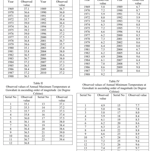
IV (A) DETERMINATION OF NaMaxT AT GUWAHATI Observed values of annual maximum Temperature at Guwahati observed during the period from 1969 to 2010 have been collected from the meteorological department of India as in [6] & [7]. These have been presented in Table I and arranged in ascending order of magnitude in Table II.
Table I
Observed values of Annual Maximum Temperature at Guwahati (in Degree Celsius) Year Observed
value Year Observed value
[image:3.595.40.551.270.780.2]1969 37.1 1989 36.7 1970 36.6 1990 36.0 1971 36.0 1991 37.4 1972 35.7 1992 39.4 1973 39.0 1993 36.4 1974 36.1 1994 37.3 1975 39.2 1995 36.3 1976 39.0 1996 37.2 1977 35.3 2000 37.5 1978 36.8 2001 36.7 1979 38.6 2002 35.7 1980 35.1 2003 37.4 1981 35.8 2004 38.0 1982 36.5 2005 36.6 1983 36.7 2006 38.0 1984 37.2 2007 37.3 1985 36.5 2008 37.3 1986 38.4 2009 38.0 1987 37.2 2010 37.2 1988 36.3
Table II
Observed values of Annual Maximum Temperature at Guwahati in ascending order of magnitude (in Degree
Celsius)
Serial No Observed
value Serial No Observed value
1 35.1 13 37.1 2 35.3 14 37.2 3 35.7 15 37.3 4 35.8 16 37.4 5 36.0 17 37.5 6 36.1 18 38.0 7 36.3 19 38.4 8 36.4 20 38.6 9 36.5 21 39.0 10 36.6 22 39.2 11 36.7 23 39.4 12 36.8
The interval values (in Degree Celsius) of the NaMaxT at
Guwahati obtained by applying the formulae (3.6), (3.9), (3.12) & (3.15) are
(36.95450 , 37.15000) , (36.93500 , 37.13000) , (36.91110 , 37.09440) & (36.88125 , 37.05625) respectively from which it can be obtained that the value of the NaMaxT at Guwahati is 37.0 Degree Celsius.
IV (B) DETERMINATION OF NaMinT AT GUWAHATI Observed values of annual minimum Temperature at Guwahati observed during the period from 1969 to 2010 have been collected from the meteorological department of India as in [6] & [7]. These have been presented in Table III and arranged in ascending order of magnitude in Table IV.
Table III
Observed values of Annual Minimum Temperature at Guwahati (in Degree Celsius)
Year Observed
value Year Observed value
1969 5.8 1989 6.7 1970 7.2 1990 8.7 1971 5.9 1991 7.4 1972 8.0 1992 5.9 1973 5.0 1993 7.8 1974 6.3 1994 8.8 1975 7.2 1995 7.5 1976 6.6 1996 9.4 1977 6.2 2000 8.5 1978 7.3 2001 8.9 1979 6.2 2002 8.6 1980 6.4 2003 8.0 1981 7.5 2004 6.7 1982 6.2 2005 8.4 1983 4.9 2006 9.6 1984 6.1 2007 6.4 1985 7.8 2008 9.7 1986 8.6 2009 9.8 1987 7.7 2010 8.6 1988 9.2
Table IV
Observed values of Annual Minimum Temperature at Guwahati in ascending order of magnitude (in Degree
Celsius)
Serial No Observed
value Serial No Observed value
1 4.9 15 7.7
2 5.0 16 7.8
3 5.8 17 8.0
4 5.9 18 8.4
5 6.1 19 8.5
6 6.2 20 8.6
7 6.3 21 8.7
8 6.4 22 8.8
9 6.6 23 8.9
The interval values (in Degree Celsius) of the NaMinT at Guwahati obtained by applying the formulae (3.6), (3.9), (3.12) & (3.15) are
(7.50370 , 7.68518) , (7,52000 , 7.70800) , (7.53913 , 7.70434) & (7.53333 , 7.70000) respectively from which it can be obtained that the value of the NaMinT at Guwahati is 7.6 Degree Celsius.
V. CONCLUSION
1. The method developed here can be summarized as follows:
(i) Arrange the distinct observed values in ascending or descending order of magnitude.
(ii) Corresponding to each observed value, compute the mean of the distinct observed all the distinct values excluding the former.
(iii) Observe the movements of the means from the highest as well as from the lowest ones and determine the value of the parameter
(iv) The value of the parameter can also be determined from the interval formed by the highest mean and the lowest mean.
(v) Confirm the correctness, of the results obtained, by repeating the process based on the observed values excluding
the extreme two observed values, the extreme four observed values, the extreme six observed values, ………. etc. respectively as required .
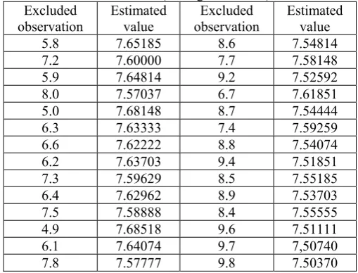
[image:4.595.297.552.153.347.2]2. The existing statistical methods of estimation yield estimates which are not free from error. However, the method developed here yield the estimate which is free from error (i.e. exactly equal to the true value of the parameter). 3. The estimated value computed by the existing methods of estimation varies if some observations are excluded and / or if some new observations are included. However, the value computed by the method developed here remains the same under this situation. Following findings (in Table V and Table VI) are some examples:
Table V
Maximum Likelihood / Minimum Variance Unbiased / Least Squares / Method of Moments / Minimum Chi Square
Estimate of the NaMaxT at Guwahati if only one
observation is excluded (in Degree Celsius) Excluded
observation
Estimated value
Excluded observation
Estimated value
37.1 37.0591 36.5 37.0864
36.6 37.0818 36.7 37.0772
36.0 37.1000 37.2 37.0545
35.7 37.1200 38.4 37.0000
39.0 36.9727 36.3 37.0955
36.1 37.1045 37.4 37.0455
39.2 36.9636 39.4 36.9545
35.3 37.1400 36.4 37.0909
36.8 37.0727 37.5 37.0409
38.6 36.9909 37.3 37.0500
35.1 37.1500 38.0 37.0182
35.8 37.1100
However, in each of these situations, the value of the
NaMaxT at Guwahati by the method developed here has been found to be 37.0 Degree Celsius.
Table VI
Maximum Likelihood / Minimum Variance Unbiased / Least Squares / Method of Moments / Minimum Chi Square
Estimate of the NaMinT at Guwahati if only one observation
is excluded (in Degree Celsius) Excluded
observation Estimated value observation Excluded Estimated value
5.8 7.65185 8.6 7.54814 7.2 7.60000 7.7 7.58148 5.9 7.64814 9.2 7.52592 8.0 7.57037 6.7 7.61851 5.0 7.68148 8.7 7.54444 6.3 7.63333 7.4 7.59259 6.6 7.62222 8.8 7.54074 6.2 7.63703 9.4 7.51851 7.3 7.59629 8.5 7.55185 6.4 7.62962 8.9 7.53703 7.5 7.58888 8.4 7.55555 4.9 7.68518 9.6 7.51111 6.1 7.64074 9.7 7,50740 7.8 7.57777 9.8 7.50370
However, in each of these situations, the value of the
NaMinT at Guwahati by the method developed here has been found to be 7.6 Degree Celsius.
REFERENCES
[1] Abraham De Moivre, “ De Mensura Sortis (Latin Version) ”, Philosophical Transaction of the Royal Society, 1711.
[2] Abraham De Moivre, “ The Doctrine of Chances ”, 1st Edition (2nd
Edition In 1738 & 3rd Edition in 1756), ISBN 0 – 8218 – 2103 – 2, 1718.
[3] Aldrich John, “ Fisher’s Inverse Probability of 1930 ”, International Statistical Review, vol. 68, pp. 155 – 172, 2000.
[4] Anders Hald, “ On the History of Maximum Likelihood in Relation to Inverse Probability and Least Squares”, Statistical Science, vol. 14, pp. 214 – 222, 1999.
[5] Birnbaum Allan, “ On the Foundations of Statistical Inference" Journal of the American Statistical Association, vol. 57, pp. 269 – 306, 1962.
[6] Dhritikesh Chakrabarty, “ Probabilistic Forecasting of Time Series “, Report of Post Doctoral Research Project (2002 – 2005), pp. 55 – 61, University Grants Commission, December 2005.
[7] Dhritikesh Chakrabarty, “ Determination of the Natural Extrema of Temperature in the context of Assam ”, Report of the Research Project (2009 – 2011), pp. 7 – 9 & 65 – 73, University Grants Commission, December 2011.
[8] Dhritikesh Chakrabarty, “ Probability: Link between the Classical Definition and the Empirical Definition ”, J. Ass. Sc. Soc., vol. 45, pp. 13 – 18, June 2005.
[9] Dhritikesh Chakrabarty, “ Bernoulli’s Definition of Probability : Special Case of Its Chakrabarty's Definition ”, Int. J. Agricult. Stat. Sci., vol. 4, no. 1, pp. 23 – 27, 2008.
[11] G. A. Barnard, “ Statistical Inference”, Journal of the Royal Statistical Society, Series B, vol. 11, pp. 115 – 149, 1949.
[12] George Marsagilia, “ Evaluating the Normal Distribution ”, Journal of Statistical Software, vol. 11, no. 4, 2004. http : / /
www.jstatsoft.org / v11/ i05 / paper.
[13] Helen M. Walker, “ De Moivre on the Law of Normal Probability ”, In Smith, David Eugene, 1985. A Source Book in Mathematics, Dover, ISBN 0 – 486 – 64690 – 4.
[14] Ivory, “ On the Method of Least Squares ”, Phil. Mag., vol. LXV, pp. 3 – 10, 1825.
[15] J. Bernoulli, “ Arts Conjectandi ”, Impensis Thurmisiorum Fratrum Basileae, 1713.
[16] Lucien Le Cam, “ Maximum likelihood — an introduction ”, ISI Review, vol. 58, no. 2, pp. 153 –171, 1990.
[17] Michiel ed. Hazewinkel, “ Normal Distribution ”, Encyclopedia of Mathematics, Springer, ISBN 978 – 1 – 55608 – 010 – 4, 2001.