Optimal negotiation strategies for agents with incomplete information

Optimal Negotiation Strategies for Agents with

Incomplete Information

S. Shaheen Fatima Michael Wooldridge Nicholas R. Jennings

Department of Computer Science,

University of Liverpool, Liverpool L69 7ZF, U.K.

S.S.Fatima, [email protected]

Department of Electronics and Computer Science, University of Southampton, Southampton SO17 1BJ, U.K.

[email protected]

Abstract. This paper analyzes the process of automated negotiation between two competitive agents that havefirm deadlines and incomplete information about their opponent. Generally speaking, the outcome of a negotiation depends on many parameters—including the agents’ preferences, their reservation limits, their attitude toward time and the strategies they use. Although in most realistic situ-ations it is not possible for agents to have complete information about each of these parameters for its opponent, it is not uncommon for agents to have partial information about some of them. Under such uncertainty, our aim is to determine how an agent can exploit its available information to select anoptimal strategy. Here, in particular, the optimal strategies are determined considering all possible ways in whichtimecan effect negotiation. Moreover, we list the conditions for convergence when both agents use their respective optimal strategies and study the effect of time on negotiation outcome.

1 Introduction

tries to maximize T (within the limit of its deadline) and the buyer tries to minimize T. In short, it is clear that agents can have different attitudes toward time.

Generally speaking, the most common time effects in bargaining situations are [6]:

– Discounting: Benefits received immediately by an agent are preferred to the same benefits received in the future.

– Bargaining Cost: The bargaining process itself may incur some cost to an agent. – Sudden Termination: An agent may have a deadline beyond which it cannot

con-tinue negotiation.

In addition to time, the outcome of a negotiation typically depends on many other parameters; such as the agents’ preferences, their reservation limits, and the strategies they use. Although in most realistic cases it is not possible for agents to have complete information about all of these parameters for its opponent, it is not uncommon to have partial information about some of them. For instance, an agent may have information about its opponent’s preferences, or its deadline. In this paper, we focus on situations where an agent has the following information about its opponent 1_:

– A set of possible values for the opponent’s reservation limit and a binary probability distribution over these values.

– A set of possible values for the opponent’s deadline and a binary probability distri-bution over these values.

With this information an agent can optimize its utility from price and time. However we do not assume that agents have full information about the preferences of their op-ponent or the strategy that they use. It is known (common knowledge) that both agents use a strategy that varies their negotiation stance with time, but the particular type of

time dependent strategythat an agent uses is not known to its opponent. Under such uncertainty, our aim is to determine how an agent can exploit the available informa-tion to select a strategy that maximises its expected utility. Moreover, when both agents have this information about one another, we determine the impact of this information on the outcome of negotiation. This analysis is important because it enables us to con-struct software agents that willoptimallynegotiate on behalf of users given their state of knowledge in a given context.

The remainder of the paper is structured in the following manner. Section 2 dis-cusses related work. Section 3 describes the basics of our negotiation model. Section 4 determines the optimal strategies for agents with incomplete information about each other. In section 5 we analyze the outcome of negotiation when both agents use their re-spective optimal strategies. Finally, in section 6 we present the conclusions and outline some avenues for future work.

2 Related Work

Game theoretic research typically deals with coordination and negotiation issues by assuming that agents have complete information about each other and then giving 1_{This information isprivatein the sense that the values that an agent has about its opponent are}

pre-computed solutions to specific problems [10]. However this perfect information assumption is limiting because uncertainty is endemic in most realistic applications. Harsanyi et al [2] give a generalized solution for two person bargaining games with incomplete information. However there is no notion of timing issues in their model. Another important model of strategic bargaining is the infinite horizon alternating offer game [11]. Since this has a unique solution, where agents agree on a split immedi-ately, it has been applied to automated negotiation [5]. However while this model takes time into consideration, it again assumes perfect information. Faratin et al.’s negotia-tion framework [1] models time as agents’ deadlines and is not based on the assumpnegotia-tion that agents have perfect information. However in this model the agent’s utility functions depend only on negotiation issues like price and quality, but are independent of time.

Perhaps the work that is most closely related to ours is that of Sandholm and Vulkan [12]. In their work on bargaining with deadlines, they consider the probability distribution over agent deadlines to be common knowledge. Specifically, they address the problem of splitting the price-surplus which is known to both agents. They show that the optimal strategy is one in which agents wait until thefirst deadline, at which point one agent concedes everything to the other. Thus agents only ever make two offers, they either demand the entire surplus or no surplus at all. This gives the entire surplus of price to the agent with the longer deadline. But because of the offers made by agents, the deadline effect completely overrides time discounting: an agent’s payoff does not change with its discounting factor. In contrast, in our work we take a binary probability distribution over agent deadlines, but we consider this to be private knowledge. In ad-dition to this, we also take a binary probability distribution over the price-surplus. But the agents do not know their opponent’s bargaining cost or discounting factor. Our opti-mal strategies too give the entire surplus of price to the agent with the longer deadline. However because of the difference in initial offers, our results bring out the difference between the effect of deadlines and time discounting. That is, the deadline effect on payoffs to agents does not suppress the effect of time discounting.

3 The Negotiation Model

We use an alternating offers negotiation protocol for our study. Let denote the buyer, the seller and let [

] denote the range of values for price that are acceptable to agent , where . A value for price that is acceptable to both and, lies between their reservation prices, i.e., in the interval [

]. The difference between

and

is theprice-surplus. Let

denote the price offered by agent to agentat time. Negotiation starts when thefirst offer is made by an agent. When an agent, say, receives an offer from agent at time, i.e.,

, it rates the offer using its utility function

. If the value of

for

at timeis greater than the value of the counter-offer agentis ready to send at time

, i.e.,

¼ with

, then agentaccepts. Otherwise a counter-offer is made. Thus the action A that agent takes at timeis defined as:

if

where

is the seller’s deadline if

from

from counter-offer

¼

¼

0.6 0.8 1 0.4

0.2 1

0.8

0.6

0.4

0.2 F

t/t_max e=50

e=0.02 e=1

(Conceder)

(Linear)

(Boulware)

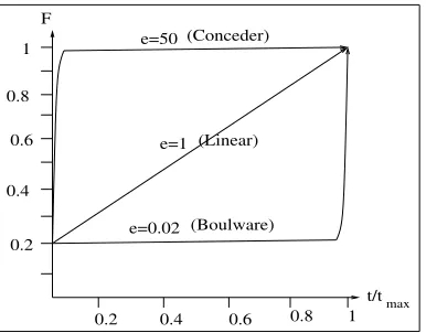
Fig. 1.Functions for the computation of

Given the fact that both agents have (different) deadlines, we assume that both agents use a strategy that varies their negotiation behaviour with respect to the pas-sage of time. Thus, time is the predominant factor used to decide which value to offer in the next negotiation move. Here such strategies are called time-dependent (from [1]). Before determining the optimal strategies (in section 4), we briefly introduce the differ-ent types of time dependdiffer-ent strategies that we consider. These strategies vary the value of price depending on the remaining negotiation time, modeled as the above defined constant . As in [1], the initial offer is a point in the interval [,

]. Agents define a constant that multiplied by the size of interval determines the price to be offered in thefirst proposal by agent. Also the offer made by agentto agent at time( ) is then modeled as a function depending on time as follows:

for the buyer

for the seller.

A wide range of time dependent functions can be defined by varying the way in which is computed. However, functions must ensure that ,

and . That is, the offer will always be between the value range, at the beginning it will give the initial constant and when the deadline is reached it will offer the reservation value. Function is defined as follows [1]:

½

These families of functions represent an infinite number of possible strategies, one for each value of. However, depending on the value of, two extreme sets show clearly different patterns of behaviour (see Fig. 1):

2. Conceder [8]: For this strategy and the agent goes to its reservation value very quickly. Whenthe price is increased linearly.

The value of a counter-offer depends on the initial price (IP) at which the agent starts negotiation, thefinal price (FP) beyond which the agent does not concede,and . Let V be a vector of these four variables, i.e., V = [IP, FP,, ]. We call this the

counter-offer vector. Let

denote

,

denote

,

and . The

negotiation outcomeis an element of , where the pair () denotes the

priceandtimeat which agreement is reached anddenotes the conflict situation.

Agents’ utility functions. The utility derived by agents depends on thefinal agreement on the priceand the duration of negotiation. However, utility from price to an agent is independent of its utility from time, i.e., the buyer always prefers a low price and the seller always prefers a high price. Thus:

We consider the following two von Neumann-Morgenstern utility functions [4] as they incorporate the effects of discounting and bargaining costs:

1. Additive form:

where

and

are unidimensional utility functions. This form is adequate when the only effect of time is a bargaining cost which is independent of thefinal out-come. We defined

as

for the buyer and

for the seller.

was defined as

. Thus when the agent

gains utility with time and when the agent loses utility with time. 2. Multiplicative form:

where, as before, and

are unidimensional utility functions. Here preferences for attribute, given the other attribute, do not depend on the level of. This form is adequate when the effects of time are bargaining cost and discounting.

was defined as before and

was defined as

. Thus when

the agent gains utility with time and when the agent loses utility with time.

Agent’s utility from conflict is defined as .

4 Optimal Negotiation Strategies

determine an optimal strategy an agent needs tofind values for V, on the basis of its negotiation environment, that maximize its utility. Since an agent’s utility depends on two parameters, price and time (see section 3), it determines the optimal price

and the optimal time

for reaching an agreement. An optimal strategy thus makes counter-offers that result in the negotiation outcome (

).

4.1 Negotiation Environments

We model the negotiation environment

for an agent , as a 9-tuple

where:

–

denotes a two element vector that contains possible values for

’s deadline such that thefirst element

is less than the second element

; –

denotes the probability that

’s deadline is

— the probability that it is

is therefore

; –

denotes the value of

on the basis of which the buyer selects an optimal strategy;

–

denotes a two element vector that contains possible values for

’s reservation price such that thefirst element

is less than the second element

; –

denotes the probability that

’s reservation price is

— the probability that it is

is therefore (

); –

denotes the value of

on the basis of which the seller selects an optimal strat-egy;

–

denotes the buyer’s deadline; –

denotes the buyer’s reservation price; –

denotes the buyer’s utility which is a function of price and time that decreases with price and either increases or decreases with time.

Elements

and

represent the information that has about

. This is the agent’s private information. Our aim is to determine optimal strategies for agents by considering all possible ways in which time can effect negotiation. Thus depending on the type of utility function

and the relation between

,

and

, the following six environments are defined:

: When

and gains utility with time, i.e.,

is an increasing function of time.

: When

and gains utility with time.

: When

and gains utility with time.

: When

and loses utility with time, i.e.,

is an decreasing function of time.

: When

and loses utility with time.

: When

and loses utility with time.

Price

s₁b _sb 2 max

Ps

Pb

s 1

P

b

P_min

max

Ps

P

P P

b

s 1 b min

Time Time

T1 T2 T s

s _{b T}s 1 Tb T2s

sb 1 _sb

2

A Price B

Fig. 2.Possible buyer strategies in environments and

4.2 Negotiation Strategies

We formally define an agent’s strategy as a function that maps its negotiation environment, , and time,, to the counter-offer vector at time ( ). Thus

. Letbe the outcome that results from strategy . is the optimal strategy for agentif it maximizes .

For any environment

,

denotes the corresponding optimal strategy. The op-timal strategies are determined for each of the above six environments. An opop-timal strategy should result in agreement at the optimal price and at the optimal time. An agent’s preference for price is independent of time, i.e., the buyer always prefers a low price and the seller always prefers a high price . We therefore determine the optimal strategy assuming

(section 4.3). This gives the optimal time for reaching agree-ment. Then for this optimal time wefind the strategy that gives the optimal price by taking the actual value of

. This is explained in section 4.4. The resulting strategy is therefore optimal in both time and price.

4.3 Optimal Strategies in Particular Environments when

This section details the optimal strategy for each of the environments noted above. The analysis is from the perspective of the buyer, although strategies for the seller can be defined analogously.

Environment

. In this environment both the deadlines of

are less than

. As both agents use time dependent tactics,will concede up to

latest by

or

. Hence it is enough if uses some strategy that concedes only up to

. Since utility increases with time until

, gets maximum utility if agreement is reached as late as possible. Since there are two possible values for the seller’s deadline, negotiation could end either at

or

and there are two possible strategies can use in this case (see Fig. 2A). It could use a strategy (

) that starts at

and approaches

at

and then makes no further concessions till

, or a strategy (

) that starts at

and approaches

at time

EU

Alpha 10

20 30

40 50 60

70

0.6 0.8 1

EU 2 Min EU₁

Avg EU₁ Max EU₁

0.4 0.2 b

b

b

b b

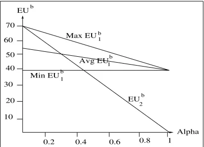
Fig. 3.Effect ofon the EU to buyer in

Boulware, ] if

and

otherwise and

Boulware,

] for all values of .

By using strategy

, gets a utility of

with probability

and a utility of

with probability (

). Note that

lies between and

depending on’s strategy. So the expected utility to ,

, from strategy

is

where

. On the other hand, if uses strategy

, it gets a utility of

with probability

and a utility of

with probability (

). So its expected utility from strategy

becomes

Turning now to an experimental evaluation of these strategies. Agent ’s utility was defined as follows2

for

for

Thus ’s utility linearly increases with price and time where

gives a value between 0 and 1. The expected utility to from any strategy depends on the following parameters:

. Let

denote the length of time interval between

and

. For all contexts we assigned

,

,

and

. In our experiments we computed the expected utility for 2_{In all the experiments reported in this section we obtained similar results for additive and}

EU

Alpha 0.6 0.8 1 0.4 0.2 20 30 50 10 40 60 70 Max EU Max EU Min EU Min EU 1 1 2 2

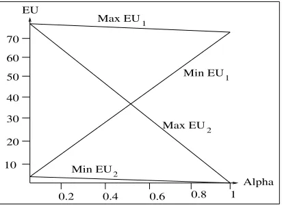
Fig. 4.Effect ofon the EU to buyer in

different values of

. For each value of

we varied

between 0 and 1 and found the

in each case. In thefirst term for

from strategy

, both parameters to

, i.e.,

and

, are constants. In the second term,

is constant but

could be any value in the interval

to

depending on the strategy that the seller uses. As a result we get a range of values for

from strategy

. Since utility to is an increasing function of time, for the same price

, gets maximum utility at

and minimum utility at

. All other possible values for

lie within this range. We therefore computed the average

for every value of

. All the parameters to in the from strategy

are constants. This gives a single value for

for every value of

. The results of this experiment for

are as shown in Fig. 3. For values of

up to 0.3, strategy

gives a higher

than the average

from strategy

. For higher values of

, the average

from

becomes higher than the from . Let

denote the value of

below which

is better than

and above which

is better than

. This value of

depends on the value of

. As we increased

, there was a corresponding increase in the value of

. A decrease in

resulted in a corresponding decrease in

. Thus the optimal strategy is when and when . Environment

. As one of the possible deadlines for the seller,

, is greater than , needs to concede up to

in order to maximize its chances of reaching an agreement. Again it could use one of two possible strategies (see Fig. 2B). A strategy

that starts at and approaches at by crossing at

, or a strategy

that starts at and approaches at , crossing

somewhere in the interval between

and

. That is,

Boulware if , Boulware, if Boulware,

for all values of. By using

Price Price

P

P

max

Pmax

b

T1 T T Time T T T2 Time s

b s 1 b

s 2 s

b

P Pminb

s 1 max

P P_maxs

b

s 1

min

P

A B

s

Fig. 5.Optimal buyer strategies when utility decreases with time

with probability

.denotes the probability that the seller crosses

prior to

. So the expected utility to from strategy

is

where

and

. If uses strategy

it gets a utility of

with probability

and a utility of

with probability

where

and

. So ’s expected utility from

becomes

In our experimental evaluation of these strategies, we get a range of values for from both strategies

and

. We assigned. The results of our experiments (for the same values of all other variables as in environment 1) are shown in Fig. 4. The

average

from strategy

was higher than the average

from

for all values of

. Note that in this case the relationship between

and

does not depend on the value of

. Thus the optimal strategy

is

for all values of

.

Environment

. Since both possible deadlines for the seller are greater than , has to use a strategy

that starts at

and concedes up to by

. Thus for all values of

!"#

In the remaining three environments ’s utility decreases with time, and it can max-imize its utility by using a strategy that ends negotiation as early as possible.

Environment

. Here

and the buyer maximizes its utility by minimizing price by conceding only up to

since it knows from its environment that

will offer

latest by

or

Price

Time P_maxs

Ps1

Pminb

Ps2

sb sb2

1

T

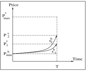
Fig. 6.Possible buyer strategies when

as early as possible. Thus ’s best strategy

is to offer

every time starting from itsfirst offer (see Fig. 5A). Thus

$#

for all values of and the counter-offers are always

.

Environment

. In this environment ’s best strategy is to offer

from the start of negotiation till

. If

is the actual deadline for the seller, negotiation would end latest

by

at price

. On the other hand, if

is the seller’s actual deadline, negotiation could continue beyond

(depending on the seller’s strategy). now has to concede up to

at the end of

since

is less than

. The strategy

is shown in Fig. 5B. Thus

$#

if

$#

if

Environment

. In this environment ’s best strategy

is to concede up to

at the beginning of negotiation since

. Thus

$#

for all values of and the counter-offers are

throughout negotiation.

4.4 Optimal Strategies in Particular Environments when The above strategies give an optimal value for if

. When

an optimal value for price needs to be determined. There are two possible values for the seller’s reservation limit,

with probability

and

with probability

. now has two possible strategies (see Fig. 6). It can concede up to

by

(strategy

) and get

an

of

EU

Alpha

0.6 0.8 1

0.4 0.2 5

10 15 20 25 30

35

Max EU

EU 1

Min EU Avg EU2

2

2 b

b

b

b

b

Fig. 7.Effect ofon the EU to buyer

or concede up to by

(strategy

) and get an of

where

.

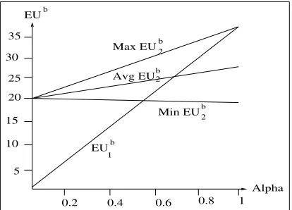
In terms of our experimental evaluation, the

from any strategy depends on the following parameters:

. We assigned

. For all contexts we assigned

and

. We varied

between 0 and 1 and computed the

for both strategies for each value of

. The results of this experiment are as shown in Fig. 7. For values of

up to 0.65 the average utility from

was higher than the

from strategy

. For values of

higher than 0.65, the

from strategy

became higher than the average

from strategy

. Let

denote the value of

below which

is better than

and above which

is better than

. Let

denote the difference between and

. The value of depends on the value of

. As we increased

there was a corresponding decrease in the value of

. The decrease in

resulted in a corresponding increase in

. Thus for

the optimal price is and for

the optimal price is .

5 Negotiation Outcomes

We now determine the outcome of negotiation when both agents use their respective optimal strategies as determined in table 1. Since the buyer and seller could either gain or lose utility with time, we have the following four possibilities:

1. Both buyer and seller gain utility with time. 2. Buyer gains and seller loses utility with time. 3. Buyer loses and seller gains utility with time. 4. Both buyer and seller lose utility with time.

Environment Optimal Strategy [ , Boulware,

] for all values of if [ , Boulware,

] for all values ofif [ , Boulware, ] if [

, Boulware, ( - )] if [

, Boulware, ] for all values of

[ , Conceder,

] for all values of [ , Conceder, ] if [

, Conceder, ( - )] if [

, Conceder, ] for all values of Table 1.Optimal Strategies for the Buyer (

denotes the optimal value for the seller’s reserva-tion price) 1. (D1) 2. (D2) 3. (D3) 4. (D4) 5. (D5) 6. (D6)

We consider the case where gains with time andloses with time and determine the outcome of negotiation for all possible orderings of deadlines. For ordering D1, let

be

’s actual deadline (see Fig. 8A). This corresponds to

for the seller and its optimal strategy is

. For agent it corresponds to

(with a high value for

) irrespective of whether its deadline is

or . Let and

denote the optimal val-ues for the seller’s minimum reservation price and buyer’s maximum reservation price respectively. Thus when uses strategy

,

uses

, and the outcome of negotiation

becomes

. On the other hand, if is

’s actual deadline (see Fig. 8B), it cor-responds to

for the seller and its optimal strategy is

. For the buyer it is and its optimal strategy is

(

is low). The negotiation outcome now becomes . In both cases, since ’s deadline is greater than’s deadline, it gets the entire surplus of price.

D2 is similar to D1 except that andare interchanged and the negotiation outcome is ( , ) when

is ’s actual deadline and ( , ) when

is ’s actual deadline (see Fig. 8C and 8D).

For D3, let

be ’s actual deadline (see Fig. 8E). This corresponds to for and its optimal strategy is

. For the buyer it is

if its deadline is and

(with

high) if its deadline is

. Using the corresponding optimal strategies, in both cases the negotiation outcome is

. If is

’s actual deadline (see Fig. 8F), this corresponds to

for

and its optimal strategy is

. Now if

is ’s actual deadline

, its optimal strategy is

and the negotiation outcome is (

,

); the entire surplus of price goes to S. But if

is ’s actual deadline

with

low), its optimal strategy gives the outcome

and the entire surplus of price goes to . For D4, let

be the seller’s actual deadline (see Fig. 8 G). This corresponds to

for the seller and its optimal strategy is

. If

or

is ’s actual deadline

T T T Ts₁ s b b_{2 1} 2

P_maxs Pob

Ps_o P_minb

T T T Ts1 s2 b b1 2

A B

Time

C _D

T

Tb b1 2T Ts s1 2 T T T Tb1 b2 s s₁ 2

Time Price _E Price _F Price _G Price H

P P

P P

s

b max

min o

o s b

T T T T₁s b_{1 2 2}s b T T T T₁s ₁b s b T T T Ts₁ b b s Ts Tb bT Ts

1 1 1

2 2 2 2 2 2

Price Price Price Price

Fig. 8.Negotiation Outcome (thick lines denote seller strategy and dotted lines buyer strategy)

then its optimal strategy is

in both cases. The negotiation outcome is

. The entire surplus of price goes to . On the other hand, if

is

’s actual deadline , its optimal strategy is

(see Fig. 8H).The optimal strategy for is

irrespective of whether its actual deadline is

or

. The corresponding outcome of negotiation is (

,

) or (

,

), and the entire surplus goes to

. In the same way the outcome of negotiation, if both agents use the optimal strategies as determined in section 3, can be found for all the remaining cases. These results are summarized in table 2.denotes the beginning of negotiation.

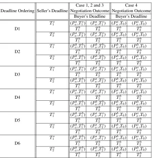
As seen from table 2, the negotiation outcome remains the same in thefirst three cases, i.e., when both agents gain utility with time, or when any one of them gains and the other loses with time. This happens because the agent that gains utility with time delays in making an offer that is acceptable to the opponent till the earliest deadline is reached. When both agents lose utility with time, they make the maximum required con-cession at the earliest opportunity, i.e. the start of negotiation. Agreement is therefore reached at the beginning of negotiation.

5.1 Conditions for convergence of optimal strategies

The values of and

are crucial in determining ’s optimal strategy. For instance in negotiation environment

, the agent’s optimal strategy

is

when

and

is

when

. Thus in order for the strategies to converge, an agent, say ’s, degree of belief

about

’s deadline must be less than

when the actual deadline for is

and it must be greater than

when the actual deadline for is

Case 1, 2 and 3 Case 4 Deadline Ordering Seller’s Deadline Negotiation Outcome Negotiation Outcome

Buyer’s Deadline Buyer’s Deadline

( , ) ( , ) ( , ) ( , ) D1 ( , ) ( , ) ( , ) ( , ) ( , ) ( , ) ( , ) ( , ) D2 ( , ) ( , ) ( , ) ( , ) ( , ) ( , ) ( , ) ( , ) D3 ( , ) ( , ) ( , ) ( , ) ( , ) ( , ) ( , ) ( , ) D4 ( , ) ( , ) ( , ) ( , ) ( , ) ( , ) ( , ) ( , ) D5 ( , ) ( , ) ( , ) ( , ) ( , ) ( , ) ( , ) ( , ) D6 ( , ) ( , ) ( , ) ( , ) Table 2.Outcome of negotiation when both agents use their respective optimal strategies

Similarly the optimal value for price depends on the value of

. For instance, for the buyer, the optimal price is

if

and it is if . Thus convergence is guaranteed only when the values of

and

satisfy the following conditions: 1. if and if

for the buyer.

2. if and if

for the seller.

3. if and if

for the buyer.

4. if and if

for the seller.

5.2 Payoffs to agents

Effect of deadlines on the payoffs. As seen from table 2, when agents have unequal deadlines, the entire surplus of price goes to the agent with the longer deadline.

Effect of discounting/bargaining costs on payoffs. When at least one agent gains

util-ity with time, agreement is reached at the earlier deadline; when both lose on time, agreement is reached toward the beginning of negotiation. Let the pair

denote the utility to andwhen both gain with time,

when gains andloses with time,

when loses andgains with time and

when both lose with time. When the effect of time on the two agents is not identical, i.e., when one of them gains utility with time and the other loses, the following result was observed. The agent that gains on time gets the same utility as compared to the case where both gain with time, i.e., for the buyer

and for the seller

. The agent that loses on time gets less utility with time gets a lower utility when compared to the case where both gain or both lose with time, i.e., for the buyer

and

and for the seller

and

.

6 Conclusions

This paper determined what the optimal negotiation strategies are for agents thatfind themselves in environments with different information states. Specifically, we consid-ered situations where agents have uncertain information about two negotiation param-eters (the opponent’s deadline and reservation limit) but do not have any information about their opponent’s bargaining cost, discounting factor or strategy. We listed condi-tions for convergence of these optimal strategies and studied the effect of time on the negotiation outcome. In the future we intend to extend our analysis to determine if this mutual strategic behavior leads to equilibria and then analyze situations where agents have limited information about other negotiation parameters like the opponent’s bar-gaining cost, its discounting factor or its strategy to compare their relative influences on the negotiation outcome.

Acknowledgments: This work was supported by the EPSRC under grant GR/M07076 (“Practical Negotiation for Electronic Commerce”).

References

1. P. Faratin, C. Sierra, and N. R. Jennings. Negotiation decision functions for autonomous agents.International Journal of Robotics and Autonomous Systems, 24(3-4):159–182, 1998. 2. J.C. Harsanyi and R. Selten. A generalized nash solution for two-person bargaining games

with incomplete information. Management Science, 18(5):80–106, January 1972.

3. N. R. Jennings, P. Faratin, A. R. Lomuscio, S. Parsons, C. Sierra, and M. Wooldridge. Au-tomated negotiation: Prospects, methods and challenges.Int Journal of Group Decision and Negotiation, 10(2):199–215, 2001.

4. R. Keeney and H. Raiffa.Decisions with Multiple Objectives: Preferences and Value Trade-offs. New York: John Wiley, 1976.

6. Z. A. Livne. The Role of Time in Negotiations. PhD thesis, Massachusetts Institute of Technology, 1979.

7. A. Lomuscio, M. Wooldridge, and N. R. Jennings. A classification scheme for negotiation in electronic commerce. In F. Dignum and C. Sierra, editors,Agent-Mediated Electronic Commerce: A European AgentLink Perspective, pages 19–33. Springer Verlag, 2001. 8. D. G. Pruitt.Negotiation Behavior. Academic Press, 1981.

9. H. Raiffa.The Art and Science of Negotiation. Harvard University Press, Cambridge, USA, 1982.

10. J. S. Rosenchein and G. Zlotkin.Rules of Encounter. MIT Press, 1994.

11. A. Rubinstein. Perfect equilibrium in a bargaining model. Econometrica, 50(1):97–109, January 1982.