doi:10.4236/wsn.2009. 14031 Published Online November 2009 (http://www.scirp.org/journal/wsn).
On the Implementation of a Probabilistic Equalizer for
Low-Cost Impulse Radio UWB in High Data Rate
Transmission
Sami MEKKI1, Jean-Luc DANGER1, Benoit MISCOPEIN2
1
Institut Telecom/Telecom Paris Tech (ENST), Paris, France
2
France Télécom R & D, Meylan Cédex, France
Email: {mekki, danger}@enst.fr, [email protected] ReceivedApril 11, 2009; revisedJune 9, 2009; accepted June 10, 2009
Abstract
This paper treats the digital design of a probabilistic energy equalizer for impulse radio (IR) UWB receiver in
high data rate (100 Mbps). The aim of this study is to bypass certain complex mathematical function as a
chi-squared distribution and reduce the computational complexity of the equalizer for a low cost hardware
implementation. As in Sub-MAP algorithm, the max* operation is investigated for complexity reduction and
tested by computer simulation with fixed point data types under 802.15.3a channel models. The obtained re-sults prove that the complexity reduction involves a very slight algorithm deterioration and still meet the low-cost constraint of the implementation.
Keywords:Impulse Radio Ultra-Wideband, Probabilistic Energy Equalizer, Inter-Symbol Interference, Chi-Squared
1. Introduction
Ultra-wideband impulse radio is considered as a promising candidate for indoor communications and wireless sensor networks, as described in [1]. Despite the numerous advantages afforded by the ultra-wideband (UWB) [1], this system faces the technological limits which brake the development of impulse radio (IR) UWB. Coherent IR-UWB reception, based on Rake receiver is limited in number of implementable Rake fingers [2]. An alternative is given by the transmitter reference (TR) method [3], however the electronic architecture is more complex as it needs analog delay lines and mixers. Non-coherent energy detection receiver is far less complex as a few components like shottky diodes and capacitors suffice. Though, the energy detection is simple to implement, transmitting impulses at high data rate leads to inter-symbol interference (ISI) which decreases the performance of the receiver [4–6]. An efficient scheme is necessary to improve the system performance.
A probabilistic energy equalizer is proposed in [7], which handles different types of interference. Besides the ISI, the proposed equalizer could manage the intra- symbol interference, called also inter-slot interference (IStI) in an pulse position modulation. Nevertheless, equalization process is mathematically
complex to implement. The problem is mainly located on the energy distribution which follows a chi-squared
distribution [8] and on the number of multiplications required by the equalizer.
array M
In this paper, the probabilistic equalizer defined in [7] is simplified by applying the Jacobi logarithm [9] where addition become max* operation (using Viterbi's notation [10]) and multiplications become additions. In order to make this possible, an approximation of the chi-squared distribution is considered and rewritten in the logarithmic domain as the probabilistic equalizer. The simplified equalizer is embedded into the iterative loop of a channel decoder which applies the Sub-MAP algorithm in the decoding process.
and the performance of the logarithmic equalizer is studied and compared to the complexity of a linear equalizer. Finally, conclusion and forthcoming work in the field are given in Section 8.
2. System Design{TC “1 Transmitter and
Receiver Design.”\f f}
We consider an IR-UWB receiver based on energy detection. Data transmission is ensured via the M - array pulse position modulation (M-PPM) over a bandwidth . Transmitting pulses over a high dispersive channel causes inter-symbol interference (ISI) and intra-symbol interference denoted as inter-slot interference (IStI). The received signal over a time symbol has the following expression
W s T ) ( ) ( = ) ( 0 = t z t x t
y n k n k
n
(1) where is an additive white Gaussian noise with variance and mean zero, and is the channel response of the transmitted symbol defined by:) (t zn
2
xnk(t)
th k n ) ( ) ( ) ( = )
(t p t A T ht
xnk nk slot (2)
where h(t) is the impulse channel response,
denotes the convolution product, is the pulse shape, is the time slot duration for an M-PPM modulation,i.e. , and takes value inaccording to transmitted symbol.
) (t p k n A, slot T
,M
slot s MT
T = 1} {0,1,
Let K denotes the number of interfering symbol assumed by the receiver, even though the real number of interfering symbol is greater. Thus for digital treatment the received signal (1) becomes a finite sum defined as:
) ( ) ( = ) ( 1 0 = t z t x t
y n k n
K
k
n
(3)The received energy per time slot in the received symbol is given by
slot
T nth
s
nt
z
nt
dt
slot T m s nT slot T m s nT m n 2 ) ( 1) ( ,
=
(
)
(
)
(4)where ( )= 1 ( ). 0
= x t
t
s K n k
k
n
Following the approach of Urkowitz [11], it was shown that the energy of a signal of duration can be represented as a sum of samples in number which is know as the degrees of freedom (DoF). Let stands for the DoF during a time slot . Thus, the energy in the slot of symbol is given by
slots
T
slot T W Tslot 2 th n L 2 th m 2 , , 2 1 = , = ( ) m n m n L mn
s z (5)
where and are respectively the sample of and in slot of symbol.
m n s , ) t m n z, ) (t n th (
sn z
th
m nth
Assuming , then the received energy follows a non-central chi-squared distribution
0 ) ( , 2 2
1
=
nm L s 2 , , 1 2 2 ) , , ( 2 1 , , 2 , , 2 1 = ) | ( m n m n L m n B m n L m n m n m n m n B I e B B
p
(6) with DoF and noncentrality parameter defined as
. The function is the -order modified Bessel function of the first kind [8]. If the noncentrality parameter is equal to zero; i.e.
; the received energy follows a central
chi-squared distribution defined as
L 2 2 =
th 1) 0 = 2 , 1 = , ( nm)L m n s B L ( ,m n B ) ( 1u IL 2 2 , 1 , 2 , ) ( 2 1 = 0) | ( m n L m n L L m n e L p
(7) where (z) is the gamma function [8].
The energy distribution is studied in next sections and simplified for hardware implementation.
3. Energy Equalization Principle
To benefit from the iterative process of a communication system, we consider a probabilistic equalizer that can be embedded into the iterative loop of a channel decoder based on SISO (Soft-Input/Soft-Output) decoding.
Thus, the considered equalizer takes the accumulated energy per slot (i.e. n,m ) and per symbol (i.e.
) , , , (
= n,1 n,2 n,M n
E ) as reference, in order to retrieve the transmitted symbol . So the detector computes a conditioned probability
regarding the interfering symbols on . It has been shown in [7] that the equalization is performed by computing
n
x
) | (En xn
p n
x
( | ) ( ) = ) | ( 1 1 = , , 1 = 1 1 k n K k m n m n M m K n x n x nn x p B x
E
p
(8) where (xnk) is the a priori probability provided by the SISO decoder and is defined in Section 2. It was also established that the set of all the
) | ( n,m Bn,m
However the smaller the number of DoF , the larger the approximation error. Due to the large bandwidth in UWB-IR, the number DoF could be big enough [16] to consider the Gaussian distribution as an approximation to the chi-squared density. For instance is around
for and . According to the previous Remark, the Gaussian approximation has the same mean and variance as the non-central chi-squared
distribution, i.e. , given by [17]:
L
2
L
2
W
30 W =3GHz
, n
E
ns Tslot =5
) ,
( 2
2 2
m N
m: possible values that could take, has a finite
cardinal. Figure 1 summarize the transmission and the receiver design under consideration.
m n
B,
In order to reduce the complexity and make the equalizer feasible, we investigate the implementation in finite precision.
Moreover the probability given by Equation (8) needs some mathematical simplifications and approximations of the probability density function (pdf) , corresponding either to the central (7) or non-central chi-squared (6) distribution. This will be investigated in the following section.
) | ( n,m Bn,m
p E
m n
B L
m ,
2 2=2
(9)
m n
B L 4 2 ,
2
2 =4 4
(10)
4. Chi-Squared Distribution Approximation
for Hardware Implementation
This can be extended to the central chi-squareddistribution by considering Bn,m=0. The chi-squared distribution defined by (7) and (6) is a
three variable function ( , and ). Thus, building a look-up table according to these parameters would occupy a great memory. For instance, if the energy distribution is coded in bits and , and are coded respectively in 14 -bit, -bit and -bit long, the space memory allocated to this look-up table would occupy Mbits (or Mbytes). This corresponds to a costly silicon area in a FPGA or ASIC technology and thus incompatible with low-cost constraints.
m n,
E Bn,m
n E
6
2
m n,
6 7
56
m
, B
2
448
Using these results and the aforementioned
assumptions, we obtain the approximation for the energy distribution (noticed p ) per slot,Bn,m0and2L>>2 as
2 2
2 2
2 2 ,
, , ,
,
2 2
) (
exp
= ) | ( ) | (
m
B p B p
m n
m n m n m n m n
E
E E
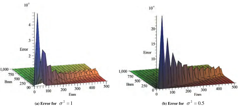
(11) Figure 2(a) shows the error measured by
for ,
and .
| ) | ( ) | (
|p En,m Bn,m p En,m Bn,m 1
=
2
0 ,m n
E Bn,m>0
An approximation for the chi-squared distribution is thus necessary. In the literature, there are some proposals for the calculation of the non-central chi-squared
[image:3.595.103.541.475.710.2]distribution [12] and the use of the normal approximation to the chi-squared distribution [13,14], but those approximations require high bit precision and are therefore too complex for digital design.
Table 1. Look-up table Input/Output size with x2
distribution.
An intuitive approximation can be found by considering the Remark in [15] which stands that when a variable is used to approximate a variable , it is equivalent to match the mean and variance of and .
Parameters Quantization size
En,m 14 bits
Bn,m 6 bits
σ2 6 bits
p(En,m|Bn,m) 7 bits
x 2 Table size 448 Mbits (56 Mbytes)
It is notably shown in [15], that a chi-squared distribution can be approximated by a Gaussian distribution.
[image:4.595.61.535.73.291.2]
(a) Error for 2=1 (b) Error for 2=0.5
Figure 2. Error measured by |p(En,m|Bn,m)p(En,m|Bn,m)| for En,m 0, Bn,m>0.
It is noticed that the error tends to zero as decreases (Figure 2 (b)). According to [7], the energy equalizer operates at ; i.e. corresponds to for a pulse energy equals to unity in coded system. So, the maximum error, considered between the
chi-squared and Gaussian distributions, is
as shown in Figure 2(a). We denote the normal function by 2
3
10 1
<
2
2=1
dB SNR=3
5
=
/2 2
2 1 = )
(t et
(12)
Using (9), (10) and (12), equation (11) can be rewritten as follows
2 2
2 , 2
2 ,
,
1 = ) | (
m B
p nm nm nm
E
E (13)
As the energy distribution is simply deduced from the normal function (t), the digital implementation can only use two look-up tables. The first one contains the values of the normal function (t),t0. The second one contains the values of the ratio 1/ x,x>0. The input/output precision of the look-up tables will be analyzed in the simulation Section according to the hardware constraints.
5. Performance of the Approximated Linear
Equalizer
In this section, computer simulations have been run to assess the performance of the linear energy equalizer with the approximated Gaussien distribution defined by (13).
The BER computation has been performed via simulations in both floating point precision and fixed point precision data types. In the firsts part of simulations, we compare the performance of the receiver with the Gaussian approximation (11) and with the exact calculation of the
chi-squared distribution in floating point precision. Second part of simulations has been run in fixed point data types with the approximated distribution.
The block fading multipath channel is generated randomly according to IEEE 802.15.3a UWB channel models [18]. Channel estimation is out of the scope of this paper. The channel state information (CSI) is assumed perfectly known at the receiver side. Nevertheless, channel parameters can be approached by the mean of the expectation-maximization (EM) algorithm as studied in [19] or by a set of a specific training sequence.
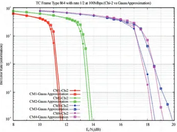
5.1. Chi-Squared Versus Gaussian Approximation Simulations in Double Precision
We consider an UWB-IR system as defined in Figure 1. Transmission is ensured by a 4-PPM modulation at
. Thus we get bits per transmitted symbol. We have implemented a duo-binary turbo code as it is defined in the standards [20,21]. This channel coder is chosen because it is suited to QPSK (quadratic phase shift keying) and 4-PPM modulations. The encoded data, at the input of the encoder, are -bit long blocks. The turbo encoder rate is and 10 iterations of the SISO decoder are performed at the receiver side. The equalizer is jointly implemented into the iterative loop of the decoder to benefit from the iterative process of the decoder. The efficiency of the energy equalizer will not
s Mbit/
100 2
be treated in this paper, the reader should refer to [7] for more details concerning the equalizer performances.
The receiver assumes that there are only two interfering symbols, i.e. K=2 and , but the real number of interfering symbols could be more. The CSI is assumed over
5 =
P
P time slots duration and not otherwise. In our case, for a data rate of Mbps, the time slot duration is , so the receiver has a perfect CSI only over . This duration is sufficient for channel models as CM1 and CM2, although their respective maximum excess delay are 80 and as it is studied in [7]. However for highly dispersive channel as CM3 and CM4 with maximum excess delay of and respectively, channel knowledge should be extended to . Nevertheless, we consider only simulations with
100
ns ns
=
K
5
ns
25
ns
200
ns
115
ns
140
3 = 2
K for the Gaussian approximation performance comparison.
It is noticed that the results with Gaussian approximation match the chi-squared performances in floating point precision even for highly dispersive channel such CM3 and CM4 with a slight degradation of performance.
5.2. Fixed Point Precision Simulations
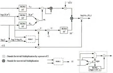
The fixed point precision is subject to hardware constraints. The duo-binary turbo coder hardware implementation is out of the scope of this paper. The digital design of the channel coder is furnished by
Turbo-Concept for an optimum efficiency [22]. The e ergy detector of UWB platform is a logarithmic one [2 guarantee the scalar value of the energy En,m for equalization, a look-up table of the function 10x
is required. Computer simulations in fixed point precision are achieved by means of the SystemC class sc_fix [24].
th ok-up ta e functions: n 3]. To
The Gaussian approximation for energy are computed rough the lo bles of th
equalization
2 = ) (
/2 x
e x
, 2
x x
g( )=1/ and x x
h( )=10 . Figure 4 sh
fix
he fractional part of the object. Hence each ob
d point simulations. Re ng the number of bits for each variable involves a significant performance decrease.
ows the Gaussian approximation computation archi- tecture for the chi-squared distribution.
According to the class sc_ of SystemC, a signed or an unsigned object are defined by two parameters: the total word length noted as wl, i.e. the total number of bits used in the type, and the integer word length noted as iwl, i.e. the number of bits that are on the left of the binary point (.) in a fixed point number. The remaining bits stand for t
ject is represented by a pair of parameters noted
> , <wl iwl .
Simulations have been carried out with different parameter sizes. Table 2 shows the word sizes of the parameters considered for the fixe
[image:5.595.119.481.425.696.2]duci
Figure 4. Approximated energy distribution architecture for the linear equalizer with x2 approximation.
[image:6.595.55.290.301.424.2]Table 3 lists the Input/Output size look–up table ne
Table 2. Parameters size definition.
Param
cessary for density computation.
eters Quantization size <wl,iwl>
m n,
log <6,2>
m n,
<14,1> m
n B, 2
> 6,2 <
<6,1>
2
m
2
> 12,2 <
2
<12,2>
) | ( n,m Bn,m
p <13,3>
) | (En xn
p <13,6>
) (xk
<4,1>
We notice that the total memory occupied by the lo
2 and 3 under the same co
Table 3. Look-up table input/output size.
Parameters Input size Output size ble size ok-up tables is lower than the chi-squared look-up table as it is described in Table 1.
Simulations according to Table
nditions as for double precision lead to the results depicted in Figure 5.
Ta (Kbits)
2 = ) (
/2 2
x
e
x <8,2> <18,0> 4.5
x x
g( )=1/ <12,2> <6,4> 24
x
x
[image:6.595.309.540.348.421.2]h( )=10 <6,2> <14,1> 0.875
[image:6.595.127.474.455.705.2]
esults in
degrade
.3. Complexity of the Linear Equalizer
he linear equalizer with a chi-squared distribution has
4 and equation (8), the amount of no
n
(14) According to the decomposition in (14),
re
R fixed point precision data types are close to those obtained in double precision with chi-squared
distribution. We notice, that even the quantization error of the energy distribution is around 1/213, which is lower than the considered maximum err 3
10 5 =
,
the receiver performances are slightly d compared to double precision simulations.
or
5
T
an expensive lookup table (Table 1). Due to the size of the ROM and its cost, the chi-squared distribution is approximated by a simple implementable function (13) with some memories.
According to Figure
n trivial multiplications in the linear domain is about
K
M K M 2)
(4 in a symbol period. We denote by on the multiplication by a power of 2
which is equivalent to a shift in hardware implementatio . The detail of multiplications is as follows1
trivial multiplicati
Mul K M Mul K k n K k Mul Mul M m n m n M m cases K M K n x n x Mtimes nn x p B x
E p 2) ( 2) ( 1 1 = 1 1) ( , , 1 = 1 1 1 ) ( ) | ( = ) |
( E
(p En e should
) |xn
quires 1
2) ( K
M K
M multiplication. W
notice that p(En|xn) is computed M times per symbol duration. T ymbol period, e total amount of multiplication is equal to (MK2)MKmultiplications. Once the number of mult
per symbol period, we divide up each terms. The a priori probability, i.e. (xnk)
hus, in a s
ipli
th
s
cation is established for (14) , will not be discussed since it is provided by th decoder. So our analysis is focused rather on the energy distribution. In the term
) | ( , , M B p
, we calculate e SISO m n m n 1 =m M timesp(n,m|Bn,m).
chitecture in Figure 4, requires
3
non-trivial multiplication. Henceperiod there is 3MK1additional multiplications on the back of (MK This leads to (4MK2)MK
multiplica by the equalizer . As example, we consider a 4-PPM modulation at With respect to the ar
K
M
2)
) | (n,m Bn,m
per symbol
p
,
tions calculated per time symbol
Mbps
0 and =2
10 K at the receiver side, this leads to
at
tiplic and a total memory of30.25Kbits
r the energy distribution c ,
, ,m nm n
s ion/
Gmul
12.8
i.e. p( |B ). We should notice that the equalizer computes the energy distribution MK1 times per time symbol. So, at 100Mbps forK=2with a 4-PPM the frequency of table access is about 3. . If we consider a hardware that runs at400MHz, level of parallelism to achieve the energy distribution is equal to 8. Thus, the total amount of mem a factor of 8, i.e.
Kbits Kbits 8=242 30.25 GHz 2 the is ory .
The next par of this paper will be focused on probabilistic equalizer com m r de the plexity reduction ean of S
ity
dware devices, t
max max = * 10 max of the
Reduct
he ex = ) , ( * 10 ab) , (ab
operation is essentially a
by the
robabilistic
plementable in uired by the
(15) ub-MAP algorithm known also as Jacobi algorithm [9].
6. Complex
io
q pe log log
n o
nsive (10 (1f the
ualizer is im area
) 10b a
10|ab|
P
req
m
Energy Equalizer
n though the defined e Eve
ha
equalizer could be decreased by simple computational method. This is made possible by computing in the logarithmic domain where only additions and comparisons operations with small memories are required. The channel decoder should operate also in the logarithmic domain, in order to get the better performance of the receiver. The decoder properties are not discussed in this paper. However, Sub-MAP algorithm, also called Max-Log-MAP or Dual Viterbi [21,10] based decoder is a good candidate for joint decoder equalizer receiver in the logarithmic domain.
As in the Sub-MAP decoding [10,25], we consider the
*
max10 function which operates in a logarithm to base 10 fined as
)
ax operation adjuste factor carried ou a lookup table read-only memory (ROM); wh utputs the correction term log(110|ab|) given the input (a b)
d by a correction ; i.e a
t by ich o
in hardware implementation. As the max property, *
is an associative operator (see APPENDIX 1 for the proo
] ), , ( [ = ) , ,
( 10* 10*
*
10 a b c max max a b c
max (16)
10 max
f):
(17)
Using the max 10operation defined in (15) ,
of the probabilistic equalizer in the logarithmic domain is For notation sim
*
plicity we consider
) (ai =
) , , ,
( * {1,
10 2
1 *
10 a a aN max i
max ,N}
the output according to Table 3 fo omputing
gi
(18 Considering the result of equation (18), it is noticed that the multiplication operations are replaced co ven by: = ) | (
logp E x
log ( | )
log ( )1 1 = , , 1 = 1 , , 1
10 nk
K k m n m n M m K n x n x n n x B p
max*
)
by mparators and adders which are costless and easy to implement. Since the equalizer output should be a probability, i.e. p(En|xn)[0,1] , a normalization process is applied as follow:
) | ( ) | ( = ) | ( n n
p x
E p
(19)where p is the normalized probability at the output of the equalizer. In the logarithmic domain normalization becomes
log
( | ) ) | ( log = ) | (log n n
n x n
n n
n x p E x p E x
E
p (20)
) | ( log ) | ( log
= p En xn max10* xn pEn xn (21)
Gaussian approximation studied in Section 4 is assumed for equalization in the logarithmic domain so that the energy distribution is feasible or implementable.
Thus, the approximated energy distribution in logarithmic domain is equal to:
n n n x n n x E x E p 10 ln 2 ) ( log 2 1 2 log 2 1 = ) | ( log 2 2 2 2 , 2 2 , , m B
p nm nm nm
(22)
One should notice that with normalization process at e output of the equalizer, the redundant constants are m
[23] which provides logarithmic energies per time slot . So, the only available data is
th
re oved. In addition, due to hardware restraint, the energy detector is a logarithm to base 10 detector as in
slot
T logEn,m, logBn,m
and log(2L2). Expending 22 in (22), we get
10 ln ) 2 (2 4 ) (
2 n,m 2
m L B )] (2
2 2 2 ,
2 , 2 m n m n B L L L
(23)
[2 log 1 ) | (
log p n,m Bn,m 2
10 ln 2.10 ) ( ) 2 (2 log 2 1 ) (2 log 2 1 )) , 2 2 (2 2 (2 log 2 2 , , 2 2 m n B L L m n m n m L B L (24)
where the symbol means “proportional to” and e function log stands for the logarithmic to base 10.
th
Rewriting (24) taking into account max*10and removing the redundant constant such as
2 ) (2 log 2
, leads to
10 ln 2.10 ) ( lo ), (2 g 2 ) , 2 2 (2 log ) 2 (2 log 2 2 , , 2 10 , , m n B L L m n m n m n m n m L L E (25) the devision part in (25) can be transformed into multi- plicationas follows: log 2 g lo 1 ) | ( log * B max Bp E
( )10
10 ln 2
2 2 ,m m n (26) where
log(2 ),log2 log 2 1 ) | ( log , 2 * 10 , , L B L max B
p nm nm nm
] log 2 log ), (2 log [ ) (2 log
= L2 max10* L2 Bn,m
(27) and n,mm2 is easily calculated as follows
(28) It is noticed that the energy distribution in logarithmic domain is achieved by the mean of two lookup tables. A first ROM for the max*10 function and a second ROM for 10x function. The memories size will be treated in sim
s used for the probabilistic equalizer complexity study.
nm L Bnm
m
n m ,
log ) 2 (2 log , log 2
, =10 10 10
the ulation Section.
The advantage of working in logarithmic domain is that the amount of multiplications is confined only on the energy distribution. Figure 6 depicts the new energy distribution architecture implemented in digital design. This architecture i
Figure 6. Energy distribution architecture for logarithmic equalizer.
7. Performance of the Logarithmic Equalizer
with the Approximated Distribution
he performances of the logarithmic equalizer with the d point prec e chi-squared distribution in
ouble precision. Reception is ensured by a logarithmic
mbols could be more.
ained
sults for hi
channel. It has been proven that for channel models CM3 and CM4, the optimal compromise is to consider
Simulations run with for CM3 and CM4 in
plex slightly
able 4. Parameters size definition.
7.1. Fixed Point DataTypes Simulation in Logarithm Domain
T
approximated distribution are simulated in fixe ision and compared to th
d
energy detector [23]. Simulations in fixed point precision are carried out by the mean of the class sc_fix of SystemC as in 5.2. Table 4 shows the word sizes of parameters considered for the fixed point simulations.
With respect to the equalizer expression (18) and to the approximated energy distribution in logarithmic domain (26), we consider two ROM types whose sizes are defined in Table 5.
Figure 7 shows the results obtained if the receiver assumes that there are only 2 interfering symbols, i.e. CSI is known only over P=5 slots, however the real number of interfering sy
We notice that for less dispersive channel such as CM1 and CM2, the results in fixed point precision data types are close to those obt in double precision with
chi-squared distribution. Regarding the re
ghly dispersive channel (CM3 and CM4), we get a loss of
1
dB
at 410 =
BER .According to [7], the receiver could be improved if the supposed number of interfering symbols are bigger than 2, especially in highly dispersive
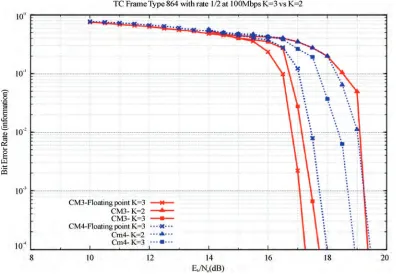
fixed point data types are depicted in Figure 8. Although the com ity is creased due to cardinal of the set {Bn,m}, i.e. |{Bn,m}|=88 for K=3 [7], the receiver is improved of 2dB for CM3 at 4
10 =
BER .
3 =
K [7].
3 =
K
in
T
Parameters Quantization size <wl,iwl>
m n,
log <6,2>
m n B,
log ,2>
) (2 log L2
<8
<7,4>
<8,4>
2
m
)
|B <7,4>
( log p n,m n,m
) | n
n x
(
logpE <6,4>
) (
logxk <6,4>
Table 5. ROM input/outp
Parameters Input size
[image:9.595.307.540.498.628.2]O size
Table size (Kbits)
ut size.
utput
= ) (x
g log(110|d|) <6,2> <4,0> 0.25
x x
h( )=10 <9,5> <8,3> 4
[image:9.595.307.541.660.719.2]Figure 7. Chi-squared float precision versus the logarithmic Gaussian approximation in fixed point precision for K=2.
Figure 8. Simulation in fixed point data types for CM3 and CM4.
7.2. Complexity of the Logarithmic Equalizer
According to the equalizer expression (18) and Figure 9, the computational complexity of the equalizer in
terms of non-trivial multiplication is equal to 1
2 K M
odulation multiplication per symbol. Thus, with 4-PPM m
at 100Mbps and K=2, we get
Regarding the memory size, the logarithmic approximati-
s ation/ .
Gmultiplic
[image:10.595.103.499.370.644.2][image:11.595.68.528.82.277.2]
Figure 9. Equalizer architecture in the logarithmic domain.
Table 6. Complexity requirement with 4-PPM and K=2.
Number of Multiplications
Function Linear x2 Linear x2 approximated Logarithmic x2 approximated
p(E
n|xn) (M+K2)MK 3.20GMultip/s (M+K2)MK 3.2 GMultip/s 0 2MK+1 6.4 GMultip/s
Total Equalizer Multiplications 4 GMultip/s
Total required mory f parallelism
) | ( n,m Bn,m
p 0 3MK+1 9.6 GMultip/s
3.2 GMultip/s 12.8 GMultip/s 6.
me
per level o 448 Mbit 30.25 Kbit 16.25 Kbit
on requ . Comp
equalizer the in the logarithm domain, i.e.
number of m
promi are imp or
instan runs at d the
que ss is e same
imated complex for it allows a compromise etween the number of multiplications and the size of
h is a Gaussian distribution instead of a leads to reduce significantly the quired memory for distribution computation. The
is to calculate all the probabilities
i domain e
ope , the computa of the
equalizer is highly reduced compared to the linear equal ver, only two ble types are required for equalizer calculation in logarithmic domain.
on fo
mmunications,” IEEE Conference on Ul-ystems and Technologies, pp. 265–269, ires 16.25Kbits
complexity ultiplications
d before, we r
aring to the linear
and the m sing for a low cost hardw
emory size, is lementation. F ce, if the hardware 400Mhz an
Ghz for th
n Table 2 fre
e
ncy of table acce 3.2
xample quote equire 8 level of parallelism to achieve the energy distribution. So the total required memory is a factor of 8; i.e. 16.25Kbits8=130Kbits) which is lower than the required memory in linear domain (242Kbits). Moreover, the required bits for each parameters in Table 4 are shorter than i .
7.3. Complexity Summary
Table 6 is the synthesize of the complexity requirement for the linear and the logarithmic equalizer with the chi-squared distribution approximation. We notice that the logarithmic equalizer with the approx energy distribution is far the less hardware implementation, since
b
the required memory for equalization calculation.
8. Conclusion
In this paper, we a have shown how a complex and costly probabilistic equalizer is simplified for digital design by using the logarithmic domain. A first simplification concerns the energy distribution whic approximated by
chi-squared. This re
second simplification
n the logarithmic by the mean of th max10*
ration. Hence tional complexity
izer. Moreo lookup ta
Computer simulations demonstrated the performance of the receiver in finite precision. It showed, that for highly dispersive channels such as CM3 and CM4, the receiver is still able to equalize and decode the transmitted informations with a slight increase in complexity.
As perspective, some operations or memories could even be simplified or reduced by the mean of polynomial approximations with a negligible loss on the receiver performance. This could be a subject of investigati r future research.
9. References
[1] L. Yang and G. B. Giannakis, “Ultra-wideband commu-nications: an idea whose time has come,” IEEE Signal Processing Magazine, Vol. 21, No. 6, pp. 26–54, No-vember 2004.
[2] J. D. Choi and W. E. Stark, “Performance of ultra-wide- band communications with suboptimal receivers in mul-tipath channels,” IEEE Journal on Selected Areas in Communications, Vol. 20, No. 9, pp. 1754–1766, De-cember 2002.
[3] R. Hoctor and H. Tomlinson, “Delay-hopped transmitted reference RF co
[image:11.595.71.522.215.321.2]d H. Arslan, “Inter-symbol interfrence
ce
ay 2005.
[Online]. Available:
systems,” ETSI EN 301 790
Proprieties
(29)
roof.
nition of we have
(30)
(31) Rewriting (29) taking on consideration (30), we get
(32)
(33) [4] V. Lottici, L. Wu, and Z. Tian, “Inter-symbol interference
mitigation in high-data-rate uwb systems,” IEEE Interna-tional Conference on Communications, pp. 4299–4304, June 2007.
[5] Y. Zhang, H. Wu, Q. Zhang, and P. Zhang, “Interference mitigation for coexistence of heterogeneous ultra-wide- band systems”, EURASIP Journal on Wireless Commu-nications and Networking, pp. 1–13, 2006.
[6] M. E. Sahin an in
[
high data rate uwb communications using energy detector receivers,” IEEE International Conference on UWB, ICU, pp. 176–179, September 2005.
[7] S. Mekki, J. L. Danger, B. Miscopein, J. Schwoerer and J. J. Boutros, “Probabilistic equalizer for ultra-wideband energy detection,” IEEE 67th Vehicular Technology Conference (VTC), pp. 1108–1112, May 2008.
[8] M. Abramowitz and I. A. Stegun, Handbook of matical Functions with Formulas, Graphs, and Mathe-matical Tables, December 1972.
[9] J. A. Erfanian and S. Pasupathy, “Low-complexity paral-lel-structure symbol-by-symbol detection for ISI chan-nels,” IEEE Pacific Rim Conf. Communications, Com-puters and Signal Processing, pp. 350–353, 1989. [10] A. J. Viterbi, “An intuitive justification and a simplified
implementation of the MAP decoder for convolutional codes,” IEEE Journal On Selected Areas In Communica-tions, Vol. 16, No. 2, pp. 260–264, February 1998. [11] H. Urkowitz, “Energy detection of unknown
determinis-tic signals,” Proceedings of the IEEE, Vol. 55, No. 4, pp. 523–531, April 1967.
[12] A. H. M. Ross, “Algorithm for calculating the noncentral chisquare distribution,” IEEE Transactions on Informa-tion Theory, Vol. 45, No. 4, pp. 1327–1333, May 1999. [13] N. C. Severo and M. Zelen, “Normal approximation to
the chisquared and non-central F probability functions,”
Biometrika, Vol. 47, No. 3/4, pp. 411–416, De mber [25] W. J. Gross and P. G. Gulak, “Simplified MAP algorithm suitable for implementation of turbo decoders,” Electron ics Letters, Vol. 34, No. 16, pp. 1577–
1960.
[14] L. Canal, “A normal approximation for the chi-square distribution,” Computational Statistics & Data Analysis, Vol. 48, No. 4, pp. 803–808, April 2005.
[15] J.-T. Zhang, “Approximate and asymptotic distributions of chi-squared-type mixtures with applications,” Journal of the American Statistical Association, Vol. 100, pp. 273–285, March 2005.
16] R. Saadane, D. Aboutajdine, A. M. Hayar, and R. Knopp, “On the estimation of the degrees of freedom of in-door UWB channel,” IEEE 61st, Vehicular Technology Con-ference (VTC), Vol. 5, pp. 3147–3151, M
[17] J. G. Proakis, Digital Communications, Second Edition, New York, McGraw Hill, 1989.
[18] J. Foerster, “Channel modeling sub-committee report final,” IEEE P802.15-02/368r5-SG3a, Tech. Rep., 18 November 2002.
[19] S. Mekki, J. L. Danger, B. Miscopein, and J. J. Boutros, “EM channel estimation in a low-cost UWB receiver based on energy detection,” IEEE International Sympo-sium on Wireless Communication Systems 2008 (ISWCS 08), pp. 214–218, October 2008.
http://samimekki.free.fr/.
[20] “Digital video broadcasting (DVB); interaction channel for satellite distribution
V.1.3.1, Tech. Rep., March 2004.
[21] “Digital video broadcasting (DVB); interaction channel for satellite distribution systems; guidelines for the use of en 301 790,” ETSI TR 101 790 V.1.2.1, Tech. Rep., January 2003.
“TC1000-xX DVB-RCS
[22] Turbo Decoder v2.1,”
Turbo-Concept, Tech. Rep., February 2005.
[23] AD8318 1 MHz to 8 GHz, 70 dB Logarithmic Detec-tor/Controller. [Online]. Available: http://www.analog. com/en/prod/0%2C2877%2CAD8318%2C00.html. [24] SystemC User’s Guide, version 2.0. [Online]. Available:
http://www.systemc.org.
1578, August 1998.
Appendix
* 10
max
] ), , ( [ = ) , ,
( 10*
* 10 *
10 abc max max ab c max
P
From the defi max10*
) 10 10 (10
log a b c
max10* (a,b,c)=
in other hand we can write
) , ( * 10 )
10 (10
log =10
10 = 10
10a b a b max ab
) 10 (10
log = ) , ,
( ( , )
* 10 *
10
c b a max c
b a
max
] ), , ( [
= 10*
*