Outdoor Universal Thermal Comfort Index Climatology for Alaska

(1)

ISSN Online: 2160-0422 ISSN Print: 2160-0414

DOI: 10.4236/acs.2019.94036 Oct. 16, 2019 558 Atmospheric and Climate Sciences

Outdoor Universal Thermal Comfort Index

Climatology for Alaska

Nicole Mölders

Geophysical Institute, Department of Atmospheric Sciences, College of Natural Science and Mathematics, University of Alaska Fairbanks, Fairbanks, USA

Abstract

Data from 456 surface meteorological sites in Alaska, eastern Russia and northwest Canada for 1979-2017 were used to model hourly universal ther-mal comfort indices (UTCIs) under consideration of Alaska-appropriate clothing. The results served to determine a high-resolution climatology of thermal comfort levels for Alaska at various temporal and spatial scales as well as the frequency of thermal stress levels. On 1979-2017 average, various degrees of cold stress occurred with highest percentage on the Alaska West Coast and along the Arctic Ocean. In the continental and Inside Passage re-gion, no thermal stress had the highest percentage of occurrence. In Interior Alaska, both strong heat and extreme cold stress occurred occasionally. At most sites and in all Alaska Köppen-Geiger bio-climate regions, the absolute range between monthly means of daily minimum and maximum UTCIs was larger than that of monthly means of daily minimum and maximum air tem-peratures. Major contributors to thermal discomfort (shortwave radiation, air temperature, moisture, wind speed) varied among bio-climate regions and in the diurnal and annual courses.

Keywords

UTCI, Universal Thermal Comfort Index, Thermal Stress in Alaska, Bio-Climate of Alaska, Thermal Stress Climatology of Alaska

1. Introduction

In recent years, the number of people exposed to the extreme elements of Alaska’s weather has increased due to population growth (almost 23% between 1994 and 2018 [1]), last-chance tourism, new activities for oil and gas explora-tion/production, and mining as well as increased Arctic shipping [2][3]. Like for How to cite this paper: Mölders, N. (2019)

Outdoor Universal Thermal Comfort Index Climatology for Alaska. Atmospheric and Climate Sciences, 9, 558-582.

https://doi.org/10.4236/acs.2019.94036 Received: September 5, 2019

Accepted: October 13, 2019 Published: October 16, 2019

http://creativecommons.org/licenses/by/4.0/

(2)

DOI: 10.4236/acs.2019.94036 559 Atmospheric and Climate Sciences

high levels of heat stress, extended exposure to extreme levels of cold stress can impact human health, reduce the efficiency of performed activities, lead to frost bite, hypothermia or even death when the exposure impairs thermoregulation

[4][5][6][7][8]. Cold stress is a significant risk factor among patients, particu-larly women with cardiovascular diseases [9]. Unlike heat waves, during which mortality raises for several days, cold spells may increase levels of mortality for several weeks [5]. Thus, as more people visit, work and/or live in Alaska and its off-shore areas, adequate public health system and urban planning require as-sessment of the outdoor thermal environmental conditions in form of climatol-ogy and frequency of occurrence at high spatial resolution.

Typically, negative influences of thermal stress on human health and perfor-mance are expressed in terms of thermal stress indices. Various thermal stress indices have been developed. They differ with respect to their input data (airflow velocity, temperature, humidity, solar radiation, etc.), rational, concepts and lo-cation [10] [11] [12] [13]. For instance, most thermal stress indices assume a standard outfit (light shirt, slacks). Some indices are valid only for air tempera-tures above (e.g. heat index, humidex for Ta > 20˚C) or below a threshold (e.g. Ta

≤ 0˚C; wind chill index, wind chill equivalent temperature index). Analytical in-dices base on the principles of thermal heat exchange between the human body and its environment; empirical indices base on human response or comfort to various environmental factors; direct indices rely on measurements like the ap-parent (AT = Ta + 0.33 × va − 0.7 × va − 4, where va is wind speed), operative or

the most commonly used Wet-Bulb Globe Temperature (WBGT = 0.567 × Ta+

0.393 × va + 3.94). The Standard Effective Temperature (SET) considers

physio-logical parameters (skin temperature and wetness). The Effective Temperature (ET) [14][15] and Physiological Equivalent Temperature (PET) were developed for indoor activity. The Mediterranean Outdoor Comfort Index (MOCI), for example, was optimized for the Cs climates [16]. The PET is based on energy balance considerations and is the output of the Munich Energy Balance Model for Individuals (MEMI). Some indices originally developed for indoor climate (e.g. SET) were adapted later to outdoor environments (OUTSET) by adding the impacts of shortwave radiation [17][18].

In studies on weather impacts on health, the mean radiant temperature Tmrt

defined as the “uniform temperature of an imaginary enclosure in which the ra-diant heat transfer from the human body equals the rara-diant heat transfer in the actual non-uniform enclosure” [19] is a better measure than ambient air tem-perature [20]. Tmrt depends, among other things, on shortwave and long-wave

radiation fluxes from all sides, body posture (sitting, standing, etc.), the absorp-tion of shortwave and long-wave radiaabsorp-tion by the human body, and wind speed. Thus, it represents the combined effects of radiant and convective heat gains/ losses for the human energy balance in the outdoors. Studies in Freiburg, Ger-many, for instance, revealed that Tmrt can differ up to 37˚C between shaded and

sunlit areas, whereas air temperature, Ta differs only 1˚C - 2˚C between the two.

(3)

rela-DOI: 10.4236/acs.2019.94036 560 Atmospheric and Climate Sciences

tions depending on Tmrt, Ta, relative humidity, va, latitude, mean annual

temper-ature, mean temperatures of the hottest and coldest months [21].

Only few studies on thermal comfort in high latitudes exist. A study in Göte-borg, Sweden (Dfb climate), for instance, showed that Tmrt can be much lower

than Ta on extremely cold days with almost no shortwave radiation reaching the

surface [22]. A study in Göteborg (57.70N, 11.94E Dfb), Luleå (65.54N, 22.11E Dfc) and Stockholm (59.35N, 18.06E Dfb) found that during clear sky condi-tions, the highest and lowest Tmrt occurred near sunlit walls and in shaded areas,

respectively; spatial variation decreased with increasing cloudiness [22]. Under cloudy conditions, highest Tmrt occurred in open areas due to high shortwave

diffuse radiation from the sky vault. While in winter, Tmrt strongly differed with

latitude, no such sensitivity occurred in summer [22]. A summer study on the thermal comfort in Apatity (67.567N, 33.4E) in the Murmansk region of Russia north of the Arctic Circle found significant spatial variation of PET during con-trast weather conditions [23].

Various studies showed that cold stress caused different responses depending on the bio-climate region. Cold spells, for instance, can cause notable and often significant increases in mortality in elderly people (65 years or older) from car-diovascular causes, especially strokes, coronary heart disease events, and respi-ratory causes in subtropical Cfa [7], in mid-latitude Cfb [4], and high latitude Dfb climate [6]. In regions with warm winters, mortality from cardiovascular diseases (CVD) increases with a given temperature decrease; in Ireland (Cfb climate), the CVD mortality rate is 45% higher in December than August, while it amounts to 28% in the much colder winters of Norway [5] (~46% in Dfc, ~26% in Cfb, ~26% in Cfc, ~1% in ET, less than 1% in Cfc climate).

Alaska still lacks an assessment of human thermal comfort at a regional scale. Weather differs widely over the state depending on the location with respect to the semi-permanent high-pressure systems, major storm tracks, elevation above sea level, distance from the coast and the presence or absence of seasonal sea-ice

[27]. Consequently, Alaska falls into several climate regions [24][28] [29][30]

(e.g. Figure 1). Unfortunately, currently available thermal stress maps like, for instance, from global simulations of various heat-stress metrics within the Community Land Model (1˚ × 1˚) [12] or derived from ERA-Interim (T255 ~79 km) [31] are too coarse to capture Alaska’s complex topographic and environ-mental and hence thermal comfort conditions.

The goals of this study were to fill this gap with a climatology and to identify regions of huge thermal hazards as well as the frequency thereof. To achieve this goal, I used near-surface meteorological observations between 1979 and 2017 (both included) to assess the thermal comfort using the Universal Thermal Com-fort Index (UTCI) model [32][33].

(4)

[image:4.595.230.521.69.223.2]

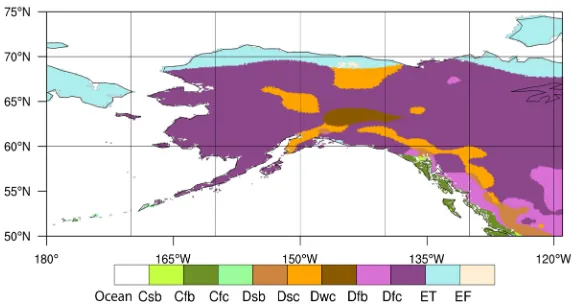
Figure 1. Köppen-Geiger classification for Alaska at 0.5˚ × 0.5˚ resolution as determined

for 1951-2000 by [24] based on datasets from the Climatic Research Unit (CRU) [25] and Global Precipitation Climatology Centre (GPCC) [26]. This resolution is between ~34.94 km (Amatignak 51.2704N, 179.1199W) and 17.82 km (Nuvuk aka Point Barrow 71.3875N, 156.4811W) in west-east and ~55.5 km in south-north direction. Except for the area of the three major cities (Anchorage 61.2181N, 149.9003W; Fairbanks 64.8378N, 147.7164W; Juneau 58.3019N, 134.4197W), the mean distance between sites exceeds 34.94 km, i.e.

gridded data include interpolated classifications.

model includes an evaluated clothing model [34][35][36] that considers human behavior of adapting insulation based on ambient air temperature in the deter-mination of thermal comfort [32][33][35][36]. This means the clothing model permits a realistic description of clothing insulation for Alaska. Furthermore, a comparison using one year of 6 am to 9 pm daily data revealed significant corre-lations (P < 0.0001) between UTCI and other heat indices (PET, PMV, SET, WBGT), and environmental parameters (e.g. dry temperature); UTCI correlated the strongest with PET (r = 0.96; r2_{= 92%) followed by WBGT (r}_{= 0.88), SET}

(r  = 0.87), and dry temperature (r  = 0.90). Note that PET and SET are based on the body thermal equation, while the thermal perception of WBGT is more sim-ilar to that of the UTCI than that of other indices [13]. See [10] and [12] for comparisons of thermal indices.

2. Experimental Design and Methodology

2.1. Data Sources and Data Processing

(5)

top of the atmosphere (TOA), Rs TOA↓, was calculated as a function of latitude,

day of the year and time of the day (for equation see e.g. [37]).

Since not all data are from operational weather monitoring, data cover time-frames of varying lengths and at different times during the period. Also some operational sites were moved or closed and new sites were set up during the pe-riod. Some sites lacked winter precipitation data or winter data at all. Thus, the available data were considered as a sample within the period following [38] and

[27].

Observational data were converted to SI units as needed. Daily accumulated precipitation was calculated from hourly or 6-hourly values when not reported as daily values. Furthermore, except for precipitation some data came at smaller time steps than an hour. These data were averaged to hourly values. Relative humidity served to determine dew-point temperatures and vice versa.

Unfortunately, in many of the datasets, the practice to just leave out hours and/or days without observations was used. However, creating a climatology requires a continuous dataset in time for 1) comparison of data from different sites at the same time, and 2) calculation of daily and monthly means as well as diurnal and annual cycles. Therefore, the data were examined for being in con-tinuous daily order for precipitation and in concon-tinuous hourly order for all other quantities. Missing data were marked as such. I discarded corrupt or bad quality data and treated them as missing. No interpolation was made for missing data in the time series.

The dataset gave cloud cover as SKC (=0 octas; clear sky), OBS or NSC (<1 octa), FEW (1 - 2 octas), SCT (3 - 4 octas), BKN (5 - 7 octas) and OVC (=8 octas; overcast). Assuming equal likelihood for all octas that belong to the same cate-gory, the respective categories’ mean was used as representative for the cloud- cover percentage, i.e. 0%, 6.25%, 18.75%, 21.875%, 68.75% and 100%, respec-tively.

For each hour without observations of solar radiation at the surface, Rs sfc↓, ,

this quantity was calculated from the incoming solar radiation at the TOA de-pendent on observed cloud cover, c as

(

3

)

, , 1 0.75

s sfc s TOA

R↓ ₌R↓ ₋ _⋅c ₍₁₎

When also no cloud-cover observations existed, cloud cover was estimated from relative humidity as [39]

1 1

1 _crit rh c

rh

− = −

− (2)

where rh is relative humidity as fraction of 1 and rhcrit = 0.7 is a critical threshold

for cloudiness to occur. Multiplication of c with 100 provides cloud cover in percent.

2.2. Calculation of the UTCI

(6)

follows the concept of an equivalent temperature. At any combination of air temperature, wind speed, radiation, and humidity, UTCI is defined as the air temperature, Ta, in the reference condition, which would elicit the same dynamic

physiological response as the actual conditions.

These reference conditions assume a metabolism of 135 W∙m−2_{, light activity}

(walking 4 km∙h−1_{), a mean radiant temperature being equal to the 2 m air}

tem-perature, a relative humidity of 50% for Ta ≤ 29˚C and water vapor pressure e =

20 hPa for Ta > 29˚C, and a 10 m wind speed, va of 0.5 m∙s−1, which corresponds

to about 0.3 m∙s−1_{at 1.1 m above ground level}_[33]_{. All other weather conditions}

are compared to this reference.

As aforementioned, the calculation of the UTCI bases on the well evaluated

[34] advanced multi-node human thermoregulation model [35]. This numerical model simulates, among others, the environmental heat exchanges, the heat and mass transfer with the body, thermoregulatory reactions of the central nervous system as well as perceptual responses [33] (Figure 2). The advanced multi-node human thermoregulation model is valid for −50˚C ≤ Ta ≤ 50˚C, −30˚C ≤ Tmrt – Ta ≤ 70˚C, 0.5 m·s−1 ≤ va ≤ 30.3 m·s−1, 5% ≤ RH ≤ 100% and water-vapor

pres-sure e < 50 hPa [33].

[image:6.595.211.538.528.704.2]

Thermo-regulation refers to the human’s ability to keep the body temperature within certain limits despite of a very different ambient temperature. When body-core temperature and/or skin temperature change, effector responses oc-cur; effector actions depend on weather conditions, clothing and activity [40] [35]. In moderate and warm environments, a person’s physiology can maintain body temperature within acceptable limits via thermoregulation; sweating and vasodilation of skin vessels occur to cool the skin by evaporation of sweat [35] [41]. In cold environments, increased convection is the main path to body-heat loss. In response, the thermoregulatory system reduces the peripheral blood flow to decrease skin temperature and to increase the thermal insulation of the skin tissue. Shivering produces heat [40].

(7)

Adequate clothing, for instance, is a behavioral effector response to thermal conditions [36]. The advanced multi-node human thermoregulation model [35]

runs in coupled mode with an adaptive clothing model [36] and predicts the dynamic thermal sensation as an equivalent temperature, the UTCI (Table 1). The model (and hence UTCI) neglects influence of physiological adaptation or acclimation.

The clothing model [36] simulates people’s adjusting their clothing to the out-side conditions. Insulation changes depending on ambient temperature. At temperatures below −20˚C, the clothing model assumes special clothing. Cloth-ing insulation values stem from data of actual behavior in the field [36]. A partial clothing approach is used. It accounts for the head and face being covered diffe-rently than the torso. It assumes the face to be exposed to the ambient air. Movement of the person and wind reduce thermal and evaporative clothing re-sistances. At ambient temperature, radiation, relative humidity and wind mod-ulate the physiological response while the clothing remains the same. The in-corporated comfort model uses physiological states (skin temperature, core temperature, sweat rate, skin wittedness, etc.) to predict thermal sensation res-ponses to steady state and transient conditions.

The difference between the UTCI value and air temperature, Ta depends on

the actual air and mean radiant temperature, Tmrt, wind speed, va and humidity

(water-vapor pressure, e or relative humidity, RH in %). The model converts the observed 10 m wind speed to body level assuming a logarithmic wind profile following [42].

The mean radiant temperature is determined following [43]

(

)

4 8 0.58

(

)

4

0.42

1.06 10

273.15 a 273.15

mrt g v g a

T T T T

D

ε × ×

= + + − −

× (3)

where Tg, va, Ta, ε and D are the globe temperature, wind speed, air temperature,

[image:7.595.211.539.580.730.2]

emissivity (0.95) and diameter of the globe. See [11] for a comparison of differ-ent methods to determine the mean radiant temperature and their impacts on UTCI (and PET) outdoor comfort levels. The globe temperature was calculated following [44].

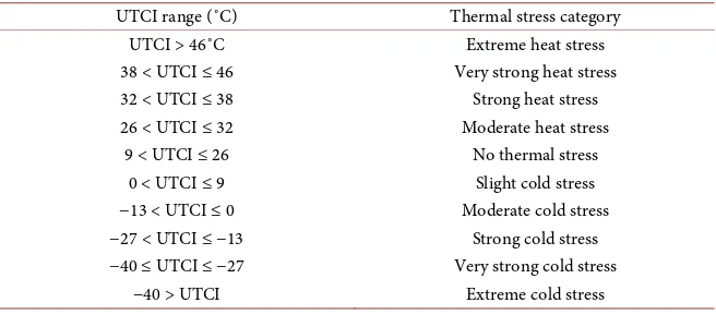
Table 1.UTCI equivalent temperatures in terms of thermal stress; values between 18 and

26˚C fall into the “thermal comfort zone”.

UTCI range (˚C) Thermal stress category

UTCI > 46˚C Extreme heat stress

38 < UTCI ≤ 46 Very strong heat stress

32 < UTCI ≤ 38 Strong heat stress

26 < UTCI ≤ 32 Moderate heat stress

9 < UTCI ≤ 26 No thermal stress

0 < UTCI ≤ 9 Slight cold stress

−13 < UTCI ≤ 0 Moderate cold stress

−27 < UTCI ≤ −13 Strong cold stress

−40 ≤ UTCI ≤ −27 Very strong cold stress

(8)

The ground surface was assumed as grass until onset of snow cover. Global albedo for shortwave and long-wave radiation was set to 0.2 for dry, snow-free conditions. Surface albedo for grass was set to 0.15 on days with at least one rain event.

A snow cover was assumed when snow depth and/or snowfall were reported. When no snow-depth data existed, a closed snow cover was assumed at latitudes north of 60˚ between November and end of March in accord with [29]. Once a snow cover existed, surface albedo was set to 0.55 (fresh snow) and 0.3 (aging snow) for days with at least one and no snow event, respectively.

2.3. Analysis

Bio-climate studies typically apply the Köppen-Geiger classification (KGC) [28] [45]. Warm temperate (C), and snow (D) climates are subdivided according to their annual precipitation (second letter) and temperature (third letter) charac-teristics. The second letters f, s, and w indicate fully-humid, dry summers, and dry winters, respectively. The third letters a, b, c, and d indicate hot, warm, cool, and extremely continental summers to describe the impacts of warmth and arid-ity on vegetation at the regional scale [28][45]. Unfortunately, many of the sur-face meteorological sites lacked or had too many missing precipitation data to calculate the KGC at the site scale. For the 370 sites with sufficient precipitation and temperature data year round, the KGC was determined using the available sample of the 1979-2017 period. Since the focus was on the thermal comfort at the actual elevation, in contrast to [28][45], the observed 2 m temperature was used, i.e. no reduction to sea-level was made.

For all sites and their available data we determined hourly UTCIs. Frequency of comfort levels, monthly means of daily minimum and maximum UTCIs, 1979-2017 monthly minimum and maximum UTCI at a site and within a bio- climate, daily and monthly means of UTCIs and their higher moments (stan-dard deviation, skewness, kurtosis) [46] as well as the percentage of hours of a given comfort level in the various months were determined from the hourly values.

For each site i with more than one year of observations, the monthly mean over the period for the jth_{month (}_{j =}_{1, 12) reads}

, 1 , ,

1 m

i j k i j k

X X

m =

=

∑

(4)

Here m is the number of hourly values in the sample of site i in all jth_months

of the period and X stands for Ta and UTCI, respectively. Analogously, the

high-er moments as well as monthly means of daily minimum Xi j, min and

maxi-mum Xi j, max and their higher moments were calculated. At a site, inter-annual

variability in monthly means was determined by the variance following [27][47] [48].

(9)

be-DOI: 10.4236/acs.2019.94036 566 Atmospheric and Climate Sciences

longing to the same bio-climate. Thus, the period-spatial mean of the jth_month

for a KGC bio-climate reads

( )

, 1 1 , ,

1 s 1 m i

KGC j i k i j k

X X

s = m i =

=

∑

₍₅₎

Here m(i) is the number of valid data in the sample at the site i during the jth

months in the period and s is the number of sites in the respective KGC bio- climate. Analogously, higher moments, period-spatial monthly means of minimum XKGC j, min and maximum XKGC j, max were determined. Consequently, the

variance describes the temporal-spatial variability within a bio-climate. For all sites with at least one year of data, the annual courses of period-monthly means, minima and maxima of both air temperature and UTCI were compared with each other. Furthermore, for each site and KGC bio-climate region the lowest (UTCImin) and highest thermal comfort level (UTCImax) were determined.

3. Results

In some continental locations, summer maximum and winter minimum tem-peratures differed more than 80 K during the period (not shown). Coastal areas without seasonal sea-ice varied the least between summer and winter tempera-tures.

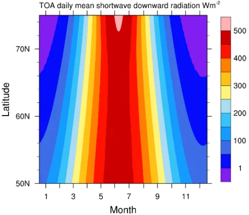
[image:9.595.250.496.477.689.2]

The annual course of solar insolation at the TOA differs strongly between North and South Alaska (Figure 3). Radiative forcing governed local weather under calm wind conditions: In winter, the low solar insolation, or even dark-ness and the snow/ice covered surfaces favored inversion formation via long- wave radiation loss; in summer, the high Sun elevation, long daylight times and strong shortwave radiation favored evaporation and eventually convection.

Figure 3. Annual evolution of daily mean incoming solar radiation at the top of the

(10)

[image:10.595.209.536.262.672.2]

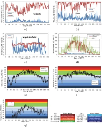
DOI: 10.4236/acs.2019.94036 567 Atmospheric and Climate Sciences Figure 4 exemplarily shows the annual courses of daily means of relative hu-midity, air temperatures, wind speeds and solar radiation at the surface for three sites: Fairbanks (64.83667N, 147.615W), Kake (56.97389N, 133.66W) and Inigok air field (70.00361N, 153.0836W). Incoming solar radiation at the surface, wind speed and relative humidity differed notably among these sites. Available short-wave radiation at the surface impacts UTCI strongly at all sites in winter. To-gether these different environmental conditions yielded thermal comfort levels that differed from the actual ambient air temperature to various degrees in the annual course.

In Alaska, actual air temperature and UTCI differed at all temporal scales. At the diurnal, monthly and annual-daily course, times existed where Ta exceeded

the UTCI and vice versa (compare e.g. Figure 4, Figure 5). Absolute differences

(a) (b)

(c) (d)

(e) (f)

(g)

Figure 4. 2015 annual course of daily means of hourly wind speed and relative humidity

(11)

(a) (b)

(c) (d)

[image:11.595.210.537.67.387.2]

(e)

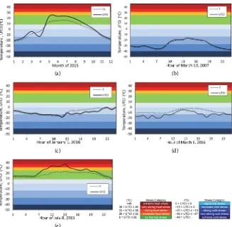
Figure 5. Fairbanks (a) monthly means in 2015, and hourly means in the diurnal course

on (b) March 13, 2007; (c) January 1, 2016; (d) March 16, 2016; (e) July 8, 2015.

between actual air temperature and UTCI varied among sites and among bio- climate regions (see Section 3.1).

Obviously, a daily or monthly climatology would exclude hourly or daily ex-tremes (cf. e.g. Figure 6). This means that with only a climatology of monthly or annual means hazardous situations may be underestimated. Therefore, the per-centage of hours in each sample for each comfort level was determined as well (see Section 3.3).

3.1. Thermal Comfort in Various Bio-Climate Regions

(12)

(a) (b)

(c) (d)

[image:12.595.209.537.71.542.2]

(e) (f)

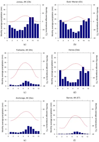
Figure 6. 1981-2010 climate monthly average precipitation and monthly mean 2 m air

temperature for selected sites in various bio-climate regions.

well. A similar distribution was obtained for 1979-2017 when determining the KGC using for the 370 sites that had sufficient air temperature and precipitation data (therefore not shown).

(13)

[image:13.595.211.533.66.207.2]

(a) (b)

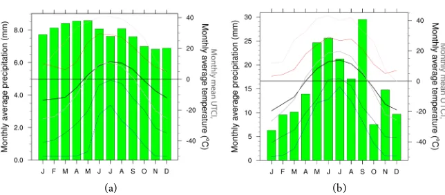
Figure 7. Annual course of 1979-2017 monthly mean precipitation (green bars), monthly

mean 2 m air temperature (black), monthly mean UTCI (gray), monthly means of mini-mum (navy) and maximini-mum (red) 2 m air temperatures and monthly means of minimini-mum (blue) and maximum (pink) UTCI at (a) Nome (64.5111N, 165.44W) and (b) Nabesna Devil Mountain (62.3986N, 142.9950W).

3.1.1. Marine West Coast Climate (Cfc, Cfb)

Along the coast of the Gulf of Alaska, frequent cyclones cause windy, wet condi-tions [29]. Thus, frigid thermal conditions are often paired with high humidity and/or high wind speeds, which can lead to wind chill. Under windy winter con-ditions blowing snow may occur as well.

Cfc bio-climate has the same annual precipitation pattern as Cfb bio-climate, but with lower temperature conditions (e.g. Figure 6(a), Figure 6(b)). Overall, in both Cfb and Cfc climates, thermal comfort levels encompassed a wider range than actual temperatures. Monthly means of daily minimum UTCI and maxi-mum air temperatures were lower than those of daily minimaxi-mum air temperature and maximum UTCI, respectively.

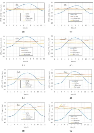
Spatially-averaged over all sites with Cfb bio-climate, the period-annual course of monthly mean UTCI spanned 21.8 K. Monthly mean UTCI was highest in July (16.3˚C ± 1.5˚C), lowest in January (−5.4˚C ± 3.2˚C), and below the freez-ing point from November to March (Figure 8(a)). Monthly mean UTCIs typi-cally exceeded monthly mean temperatures from May to August (Figure 8(b)). The opposite was true from October to March. Together these findings suggest that on average, May to September saw no thermal stress, while moderate ther-mal stress occurred from November to March. The lowest minimum and highest maximum 1979-2017 UTCI-values were −12.9˚C and 18.6˚C, respectively (Table 2).

On period-average over all Cfc sites, the difference between the highest and lowest mean monthly UTCIs in the period-annual course was 25.6 K, i.e. larger than in Cfb bio-climate. January and July had the lowest (−14.7˚C) and highest monthly mean UTCIs (11.0˚C). On average, at least moderate cold stress

oc-curred from October to April (Figure 8(b)). Monthly mean UTCIs exceeded

(14)

(a) (b)

(c) (d)

(e) (f)

[image:14.595.210.537.66.529.2]

(g) (h)

Figure 8. Bio-climate period-spatial monthly mean, standard deviation (StDev), skewness

and kurtosis of UTCI for (a) Cfb; (b) Cfc; (c) Dfb; (d) Dfc; (e) Dwb; (f) Dwc; (g) Dsc and (h) ET bio climate.

zone. Typically, slight cold stress occurred from April to June and in September. During the period, the lowest minimum and highest maximum UTCI were −20.6˚C and 14.9˚C, respectively (Table 2).

(15)

[image:15.595.211.538.162.468.2]

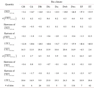
Table 2. Minimum UTCIKGCmin and maximum UTCIKGCmax universal thermal comfort

indices, standard deviation, σ, skewness, and kurtosis calculated over all months and sites of available data for a respective bio-climate region as well as the minimum UTCImin and maximum hourly universal thermal comfort index UTCImax within the respective bio- climate region during the period. Here # is the number of sites having hourly data for all months of at least one year. Only sites on land are considered.

Quantity Bio-climate

Cfb Cfc Dfb Dfc Dsc Dwb Dwc EF ET

min KGC

UTCI −5.4 −14.7 −14.0 −21.1 −23.3 −18.0 −24.8 −37.3 −33.9

(

min

)

σ UTCI_KGC 3.2 4.2 6.2 8.6 8.2 6.3 6.6 9.3 4.5

Skewness of

min KGC

UTCI −0.8 −0.5 −0.1 0.1 0.1 0.5 0.4 0.2 1.2

Kurtosis of

(

UTCIKGCmin

)

−0.2 −1.8 −1.1 −0.4 −2.0 −1.1 −0.6 −1.3 12.5

min KGC

UTCI −12.8 −20.6 −28.5 −40.6 −31.7 −27.3 −37.9 −45.6 −40.0

max KGC

UTCI 16.3 11.0 18.6 15.9 16.6 20.6 14.9 −4.5 2.6

(

max

)

σ UTCI_KGC 1.5 2.7 4.5 5.0 5.9 5.8 5.1 16.3 4.0

Skewness of

max KGC

UTCI −0.4 0.8 0.5 −0.7 −0.1 −0.3 0.3 −0.1 0.0

Kurtosis of

max KGC

UTCI −1.4 −1.7 −0.1 0.2 −1.8 −1.1 0.3 −2.3 0.7

max KGC

UTCI 18.6 14.9 9.9 25.0 19.5 24.3 34 10.9 18.6

# of sites 14 4 26 111 5 11 114 7 62

inter-annual variance was largest in January and smallest in September (cf. Fig-ure 8(a), Figure 8(b)).

The pattern in inter-annual variability can be explained as follows: High UTCI values are associated with low cloudiness, high-pressure situations. Under such synoptic situations, shortwave radiation, calm winds and topography govern the temperature and moisture conditions over a large area [37][49]. However, low UTCI values occur under cyclonic conditions. Wind speeds, cloudiness, humid-ity and temperatures strongly differ before and after a frontal passage. The sulting strong gradients in meteorological parameters over the bio-climate re-gion yield great variability in UTCI.

3.1.2. Humid Continental Climate (Dfb, Dwb)

Dfb and Dwb climates are hemi-boreal [28]. Temperatures of the four warmest months are 10˚C or above, but less than 22˚C. These bio-climates mainly differ by the timing of precipitation (not shown).

(16)

on period-spatial average, January and July had the lowest (−14.0˚C) and highest monthly mean UTCI (18.6˚C), respectively. Monthly mean UTCIs indicated at least moderate cold stress from November to March (Figure 8(c)). Lowest and highest UTCIs obtained at sites with Dfb climate were −28.5˚C and 9.9˚C (Table 2) indicating strong and no thermal stress for the extremes, respectively.

In Dwb climate, on period-spatial average, January and July had the lowest (−18.0˚C; strong thermal stress) and highest monthly mean UTCIs (20.6˚C; no thermal stress). This wider range in UTCI values in Dwb than in Dfb bio-climate results from the enhanced humidity due to winter precipitation and less humid-ity in summer. In Dwb bio-climate, the lowest and highest UTCI were −27.3˚C (strong thermal stress) and 24.3˚C (no thermal stress), respectively (Table 2). Monthly mean UTCI values indicated moderate or worse cold stress from Octo-ber to March (Figure 8(e)).

In both Dfb and Dwb bio-climates, spatial-inter-annual variance in monthly mean UTCIs was lowest in September. In Dfc bio-climate, this variability was notably higher from November to March than in the other months, largest in December followed by November and February. In Dwb bio-climate, January saw the highest spatial-inter-annual variance followed by November and Febru-ary. The strong decrease and increase of solar radiation with latitude (Figure 3) in these months are major reasons. In summer, latitudinal differences in solar radiation are much smaller over these regions.

3.1.3. Continental Subarctic Climate (Dfc, Dwc)

Dfc and Dwc climates are colder than Dfb and Dwb climates. Again, Dfc and Dwc climate are the same with respect to their temperature thresholds, but differ by the timing of precipitation.

The vicinity to the Canadian High leads to mostly calm or no wind conditions in Interior Alaska. In Dfc bio-climate, highest and lowest period-spatial monthly means of UTCI differed 35.9 K. Typically, January and July had the lowest (−20.6˚C; strong cold stress) and highest monthly mean UTCIs (15.3˚C; no thermal stress), respectively. Averaged over the period and all Dfc sites, monthly mean UTCIs indicated various degrees of cold stress from October to April with at least moderate cold stress (Figure 8(d)). The lowest and highest UTCI ob-tained at sites with Dfc bio-climate were −40.7˚C (extreme cold stress) and 25.0˚C (no thermal stress), respectively (Table 2).

Due to the high humidity associated with winter precipitation, highest and lowest period-spatial monthly mean UTCI differed 39.8 K in Dwc bio-climate. On period-spatial average, the lowest minimum (−24.8˚C) and highest maxi-mum monthly mean UTCIs (14.9˚C) occurred in January and July, respectively. Monthly mean UTCIs were below 0˚C from October to April (Figure 8(f)). The lowest and highest UTCIs calculated for sites with Dwc bio-climate were −37.9˚C and 34.3˚C, respectively (Table 2). This means both very strong cold stress and strong heat stress occurred.

(17)

preci-DOI: 10.4236/acs.2019.94036 574 Atmospheric and Climate Sciences

pitation amount in August; cf. Figure 6(c)) and Dwc (dry summer) bio-climate, August UTCIs showed the least variability in space and time. In Dfc bio-climate, highest spatial-inter-annual variance in thermal comfort conditions occurred in March followed by April (melting season), while in Dwc bio-climate, highest spatial-inter-annual variance occurred in April followed by March, May, and February.

3.1.4. Mediterranean-Influenced Subarctic Climate (Dsc)

At the few sites with Dsc bio-climate, highest and lowest period-spatial monthly mean UTCIs differed 39.9 K. On period-spatial average, the minimum (−23.3˚C) and maximum monthly mean UTCIs (16.6˚C) occurred in January and July, re-spectively. Monthly mean UTCIs stayed below freezing from October to April (Figure 8(g)). The humidity and wind from the ocean caused moderate to strong cold stress during these months. During 1979-2017, the lowest and high-est UTCI in Dsc climate were −31.7˚C (very strong cold stress) and 19.5˚C (no thermal stress), respectively (Table 2). The high heat capacity of the ocean de-lays warm-up in spring and may result in cool sea-breezes keeping summers comfortable. In fall, the high heat capacity of the ocean contributes to mild con-ditions. The winds and high humidity yield cold stress of various degrees in winter and spring.

Spatial-inter-annual variance in UTCIs was highest in April caused by occa-sional late snowfall and the presence or absence of sea-ice close to the shores. During June to September spatial-inter-annual variance in thermal conditions was notably lower than during the cold season with September having the least variability. The strong inter-annual variability of thermal comfort in winter can be attributed to the inter-annual variability in storm tracks and extension/location of high-pressure systems. Storms from the south advect Mediterranean warm air masses, while a strong high-pressure system can advect Arctic cold air from the Interior and Yukon Territory.

3.1.5. Tundra and Ice-Cap Climate (ET, EF)

As can be seen in Figure 3, solar insolation gradually decreases northward over the tundra leading to no insolation from late November to end of January in the northernmost areas. During that time, long-wave radiation loss governs the energy budget and thermal comfort. Once the Sun comes back, the high albedo of snow reflects huge amounts of shortwave radiation that reaches the surface.

In ET bio-climate, monthly mean UTCI were above freezing only in July meaning still slight cold stress on average. Very strong cold stress with monthly mean UTCIs below −30˚C occurred from December to March.

(18)

In ET bio-climate, spatial-inter-annual variance in monthly mean UTCI was highest in March and lowest in August (Figure 8(h)). Skewness and kurtosis were highest in February when the Sun comes again above the horizon. Both skewness and kurtosis had a secondary maximum in November when the solar insolation reached zero (Figure 8(h), Figure 3).

In EF climate, spatial-inter-annual variance in monthly UTCIs was least in November to January, largest in June and marginally less in May. In the former months, long-wave radiation dominates, while in June shortwave radiation at the TOA is the largest (Figure 3). The high inter-annual variability results from variability in cloudiness and hence shortwave radiation reaching the surface. Skewness ranged between −0.3 (September) and 0.5 (February). Kurtosis was negative in all months with higher absolute values in summer than winter.

3.2. Climatology of Alaska Thermal Comfort

In this analysis, for each of the 456 sites, its total available data were taken as 100%. Figure 9 shows for each of the sites the most often occurring thermal comfort level and the percentage of hours it occurred. No thermal stress existed between 20% and 30% of the time in the Interior of Alaska as well as 25% to 40% of the time in the Inside Passage. Along the Gulf of Alaska, slight and moderate cold stress dominated the thermal comfort levels. In the Aleutians, moderate and strong cold stress were the most frequent conditions governing the thermal comfort levels 15% to 35% of the time.

[image:18.595.211.538.457.671.2]

Crews on oil and gas platforms in the Chukchi and Beaufort Seas were ex-posed to very strong or strong cold stress 45% to 50% of the time (Figure 9,

Figure 10). Slight cold stress existed in the Chukchi and Beaufort Seas up to 20%

Figure 9. Map showing the most often occuring thermal comfort conditions at a site

(19)

[image:19.595.212.538.67.395.2]

Figure 10. Interpolated maps of percent of occurrence of various thermal comfort

condi-tions for Alaska. Strong and extreme heat stress occur less than 5% of the time in Alaska (therefore not shown).

of the time. In the eastern Beaufort Sea, moderate cold stress occurred up to 35% of the time (Figure 9). Note that ships cruise in these seas from June to late Oc-tober [2][50].

The continental regions of Alaska (and the Yukon Territory) had slight heat stress up to 10%. In some places, strong heat stress occurred on occasions as well. The continental regions of Alaska experienced a higher fraction of time with very strong cold stress than those along the Gulf of Alaska or in the Aleu-tian (Figure 9). Along the Alaska West Coast, the fraction of time with very strong cold stress increased with latitude reaching up to 25% on the North Slope. This means the low or lack of insolation played a key role for deep winter ther-mal comfort. Note that pockets with even more hours of very strong cold stress occurred.

4. Discussion, Conclusions and Outlook

(20)

in-DOI: 10.4236/acs.2019.94036 577 Atmospheric and Climate Sciences

cludes maps of the percentage of time that the various thermal comfort levels occurred. Furthermore, it also includes the mean thermal comfort in Alaska’s Köppen-Geiger bio-climates.

The 1979-2017 thermal climatology of Alaska reveals the following. At most sites and in all bio-climates in Alaska, thermal comfort levels encompassed a wider range than actual air temperatures. In general, differences between actual air temperature and UTCI varied with the time of the day, day and month of the year (i.e. shortwave radiation reaching the ground, long-wave radiation loss, wind speed, humidity). The various bio-climates differed in the range of thermal comfort levels as well as timing of when monthly means of air temperatures ex-ceeded those of UTCI and vice versa. However, at most sites, monthly mean UTCI values exceeded monthly mean air temperatures in summer, while the opposite was true in winter. Typically, monthly means of daily minimum UTCI were lower than monthly means of daily minimum air temperature; the opposite was true for the maxima.

The thermal conditions with the highest percentage of occurrence ranged from slight cold stress to very strong cold stress except for Interior Alaska and along the Inside Passage. In Interior Alaska and along the Inside Passage, no thermal stress had the highest percentage of occurrence. Nevertheless, cold stress of different degrees dominated overall in these two regions. These two regions and the very continental Dwc bio-climate had the widest range of thermal con-ditions. However, in the former two regions, thermal comfort levels reached from extreme cold to very strong heat stress, while they reached from very strong cold stress to strong heat stress in Dwc bio-climate. However, the fre-quency of occurrence was marginal for these extremes in all three regions.

Along the coasts of West and North Alaska and the northern Gulf of Alaska some degrees of cold stress had the largest percentage of occurrence. Along the northern Gulf of Alaska, wind and enhanced humidity from the ocean were notable contributors to low UTCI levels. Along the Bering Sea coast north of the Arctic Circle and along the coast of the Arctic Ocean, the low or lack of solar insolation in combination with long-wave radiation loss in winter and windy, humid conditions in summer led to on average uncomfortable thermal condi-tions year round.

Except for Dwc climate, spatial-inter-annual variability in thermal comfort levels was higher for the cold than warm thermal range, but differed in timing of minima and maxima among bio-climates. In Dwc bio-climate, spatial-inter-annual variability in UTCI was larger in the first than second half of the year.

In ET climate, the skewness and kurtosis of UTCI increased strongly in Feb-ruary and November due to the incremental northward increase and decrease, respectively, of shortwave radiation reaching the surface. In all other bio-climates, skewness and kurtosis showed only marginal differences among months.

(21)

percep-DOI: 10.4236/acs.2019.94036 578 Atmospheric and Climate Sciences

tions of thermal-environmental conditions, and effector behavior. Studies com-paring the clothing behavior of residents with similar summer UTCI-ranges showed that those living in Melbourne wore more clothing (0.1 clo) than those in Hong Kong [52]. This means that the Alaska thermal comfort climatology might underestimate the thermal stress of new residents and tourists.

In the regions of increased exploration, oil and gas production, strong to very strong cold stress dominated. Thermal comfort rarely exceeded slight cold stress. Similar was true for the regions of increased shipping. Based on these findings one may conclude that here the capacities for treatment of cold stress related symptoms have to be extended as the population, ship and air traffic increases on the North Slope and its coastal waters. The increasing tourism for aurora watching, dog-mushing, hiking, kayaking, fishing, boating etc. in Interior Alaska will require expansion of capacity to treat patients with cold and heat thermal stress.

The more than 23% growth in Alaska’s population mainly increased the out-skirts of the three major cities (Anchorage, Fairbanks, Juneau). Recent studies showed that increasing urbanization and improved urban planning, among oth-er things, altoth-ered the thoth-ermal stress in European cities of diffoth-erent background climates over time [53]. Given the few urban sites in Alaska, of which many have only short time series, the assessment of small-scale differences in thermal com-fort and planning for its improvement remain a challenge. Thus, the develop-ment of urban thermal comfort models is an urgent need as well.

Major challenges in determining a thermal comfort climatology for Alaska were the quantity and quality of available data. While at a few sites, over 100 years of data exist [29], the number of available sites and the spatial resolution of sites were too coarse for a meaning-full spatial climatology starting at that time. Furthermore, some of these early time series only reported daily maxima, mini-ma and means, i.e. they had a coarse temporal resolution. Thus, using the data from 1979 to 2017 was a compromise between sufficient spatial resolution, num-ber of sites and length of the time series.

However, when looking at a limited timeframe, extreme events with low probability of occurrence may be missed. For instance, the highest and lowest recorded temperature since onset of recording were 37.8˚C (Ft. Yukon, June 27 1915) and −62.2˚C (Prospector Creek, January 23, 1971), respectively [29]. This means that the 1979-2017 sample missed these and probably other local ex-tremes.

(22)

Acknowledgements

I thank G. Kramm and the anonymous reviewers for fruitful comments and discussion. My thanks also go to the many PIs and their co-workers of the vari-ous research projects that made their data available in the data archives used in this study. Data stem from the National Centers for Environmental Information (NCEI), National Climatic Data Center (NCDC), United States Geological Sur-vey (USGS), Atmospheric Radiation Measurements (ARM), Water Engineering Research Center (WERC), Bureau of Ocean Energy Management (BOEM) and Western Region Climate Center (WRCC). The model to calculate UTCI stems from P. Bröde. Financial support came from the State of Alaska.

Conflicts of Interest

The author declares no conflicts of interest regarding the publication of this pa-per.

References

[1] US Census Bureau (2019) 2018 National Population Projections.

[2] Arctic-Council (2009) Arctic Marine Shipping Assessment 2009 Report. 194 p. [3] Mölders, N. and Gende, S. (2016) On the Limits to Manage Air-Quality in Glacier

Bay. Journal of Environmental Protection, 7, 1923-1955.

https://doi.org/10.4236/jep.2016.712151

[4] Laschewski, G. and Jendritzky, G. (2002) Effects of the Thermal Environment on Human Health: An Investigation of 30 Years of Daily Mortality Data from SW Germany. Climate Research, 21, 91-103. https://doi.org/10.3354/cr021091

[5] Mercer, J.B. (2003) Cold—An Underrated Risk Factor for Health. Environmental Research, 92, 8-13. https://doi.org/10.1016/S0013-9351(02)00009-9

[6] Kysely, J., Pokorna, L., Kyncl, J. and Kriz, B. (2009) Excess Cardiovascular Mortality Associated with Cold Spells in the Czech Republic. BMC Public Health, 9, 19.

https://doi.org/10.1186/1471-2458-9-19

[7] Ma, W., Yang, C., Chu, C., Li, T., Tan, J. and Kan, H. (2013) The Impact of the 2008 Cold Spell on Mortality in Shanghai, China. International Journal of Biometeorolo-gy, 57, 179-184.https://doi.org/10.1007/s00484-012-0545-7

[8] Di Napoli, C., Pappenberger, F. and Cloke, H.L. (2018) Assessing Heat-Related Health Risk in Europe via the Universal Thermal Climate Index (UTCI). Interna-tional Journal of Biometeorology, 62, 1155-1165.

https://doi.org/10.1007/s00484-018-1518-2

[9] Skutecki, R., Jalali, R., Dragańska, E., Cymes, I., Romaszko, J. and Glińska-Lewczuk, K. (2019) UTCI as a Bio-Meteorological Tool in the Assessment of Cold-Induced Stress as a Risk Factor for Hypertension. Science of the Total Environment, 688, 970-975. https://doi.org/10.1016/j.scitotenv.2019.06.280

[10] Blazejczyk, K., Epstein, Y., Jendritzky, G., Staiger, H. and Tinz, B. (2012) Compari-son of UTCI to Selected Thermal Indices. International Journal of Biometeorology, 56, 515-535. https://doi.org/10.1007/s00484-011-0453-2

(23)

DOI: 10.4236/acs.2019.94036 580 Atmospheric and Climate Sciences https://doi.org/10.1007/s00484-013-0777-1

[12] Buzan, J.R., Oleson, K. and Huber, M. (2015) Implementation and Comparison of a Suite of Heat Stress Metrics within the Community Land Model Version 4.5. Geos-cientific Model Development, 8, 151-170. https://doi.org/10.5194/gmd-8-151-2015

[13] Zare, S., Hasheminejad, N., Shirvan, H.E., Hemmatjo, R., Sarebanzadeh, K. and Ahmadi, S. (2018) Comparing Universal Thermal Climate Index (UTCI) with Se-lected Thermal Indices/Environmental Parameters During 12 Months of the Year.

Weather and Climate Extremes, 19, 49-57.

https://doi.org/10.1016/j.wace.2018.01.004

[14] Houghton, F.C. and Yaglou, C.P. (1923) Determining Equal Comfort Lines. J. Am. Soc. Heating and Ventilation in England, 29, 165-176.

[15] Fountain, M. and Huizenga, C. (1995) A Thermal Sensation Model for Use by the Engineering Profession-Results of Cooperative Research between the American So-ciety of Heating, Refrigeration, and Air-Conditioning Engineers, Inc. and Environ-mental Analytics. 1-55.

[16] Salata, F., Golasi, I., De Lieto Vollaro, R. and De Lieto Vollaro, A. (2016) Outdoor Thermal Comfort in the Mediterranean Area. A Transversal Study in Rome, Italy.

Building and Environment, 96, 46-61.

https://doi.org/10.1016/j.buildenv.2015.11.023

[17] Jendritzky, G. and Nubler, W. (1981) A Model Analyzing the Urban Thermal Envi-ronment in Physiologically Significant Terms. Archives of Meteorology and Geo-physical Bioclimatology, 29, 313-326. https://doi.org/10.1007/BF02263308

[18] Pickup, J. and De Dear, R. (2000) An Outdoor Thermal Comfort Index (OUT- SET*)-Part I—The Model and Its Assumptions.5th International Congress of Bio-meteorology and International Conference on Urban Climatology, Macquarie Uni-versity, Sydney, 279-283.

[19] ASHRAE (2001) ASHRAE Fundamentals Handbook 2001. SI Edition. 892 p. [20] Thorsson, S., Lindqvist, M. and Lindqvist, S. (2004) Thermal Bioclimatic

Condi-tions and Patterns of Behaviour in an Urban Park in Göteborg, Sweden. Interna-tional Journal of Biometeorology, 48, 149-156.

https://doi.org/10.1007/s00484-003-0189-8

[21] Golasi, I., Salata, F., De Lieto Vollaro, E. and Coppi, M. (2018) Complying with the Demand of Standardization in Outdoor Thermal Comfort: A First Approach to the Global Outdoor Comfort Index (GOCI). Building and Environment, 130, 104-119.

[22] Lindberg, F., Holmer, B., Thorsson, S. and Rayner, D. (2013) Characteristics of the Mean Radiant Temperature in High Latitude Cities-Implications for Sensitive Cli-mate Planning Applications. International Journal of Biometeorology, 58, 613-627.

https://doi.org/10.1007/s00484-013-0638-y

[23] Gommershtadt, O., Konstantinov, P., Varentsov, M. and Baklanov, A. (2020) Mod-eling Technology for Assessment of Summer Thermal Comfort Conditions of Arc-tic City on Microscale: Application for City of Apatity. In: Vasenev, V., Dovletya-rova, E., Cheng, Z., Valentini, R. and Calfapietra, C., Eds., Green Technologies and Infrastructure to Enhance Urban Ecosystem Services. SSC 2018, Springer Geogra-phy, Springer, Cham, 66-75. https://doi.org/10.1007/978-3-030-16091-3_10

[24] Kottek, M., Grieser, J., Beck, C., Rudolf, B. and Rubel, F. (2006) World Map of the Köppen-Geiger Climate Classification Updated. Meteorologische Zeitschrift, 15, 259-263.https://doi.org/10.1127/0941-2948/2006/0130

(24)

Grids of Monthly Climatic Observations—The CRU TS3.10 Dataset. International Journal of Climatology, 34, 623-642. https://doi.org/10.1002/joc.3711

[26] Schneider, U., Fuchs, T., Meyer-Christoffer, A. and Rudolf, B. (2008) Global Preci-pitation Analysis Products of the GPCC. Global PreciPreci-pitation Climatology Centre (GPCC), Deutscher Wetterdienst, Offenbach, Germany, 12 p.

[27] Mölders, N. and Kramm, G. (2018) Climatology of Air Quality in Arctic Cities-In- ventory and Assessment. Open Journal of Air Pollution, 7, 48-93.

https://doi.org/10.4236/ojap.2018.71004

[28] Geiger, R. (1961) Überarbeitete Neuausgabe Von Geiger, R. Köppen Geiger/Klima der Erde. (Wandkarte 1:16 Mill.).

[29] Shulski, M. and Wendler, G. (2007) The Climate of Alaska. 216 p.

[30] Bieniek, P.A., Walsh, J.E., Thoman, R.L. and Bhatt, U.S. (2014) Using Climate Divi-sions to Analyze Variations and Trends in Alaska Temperature and Precipitation.

Journal of Climate, 27, 2800-2818. https://doi.org/10.1175/JCLI-D-13-00342.1

[31] Pappenberger, F., Jendritzky, G., Staiger, H., Dutra, E., Di Giuseppe, F., Richardson, D.S. and Cloke, H.L. (2015) Global Forecasting of Thermal Health Hazards: The Skill of Probabilistic Predictions of the Universal Thermal Climate Index (UTCI).

International Journal of Biometeorology, 59, 311-323.

https://doi.org/10.1007/s00484-014-0843-3

[32] Jendritzky, G., Bröde, P., Fiala, D., Habvenith, G., Weihs, P., Batchvarova, E. and Dedear, R. (2009) Der Thermische Klimaindex UTCI. 96-101.

[33] Bröde, P., Fiala, D., Błażejczyk, K., Holmér, I., Jendritzky, G., Kampmann, B., Tinz, B. and Havenith, G. (2012) Deriving the Operational Procedure for the Universal Thermal Climate Index (UTCI). International Journal of Biometeorology, 56, 481- 494. https://doi.org/10.1007/s00484-011-0454-1

[34] Psikuta, A., Fiala, D., Laschewski, G., Jendritzky, G., Richards, M., Błażejczyk, K., Mekjavič, I., Rintamäki, H., De Dear, R. and Havenith, G. (2012) Validation of the Fiala Multi-Node Thermophysiological Model for UTCI Application. International Journal of Biometeorology, 56, 443-460. https://doi.org/10.1007/s00484-011-0450-5

[35] Fiala, D., Havenith, G., Bröde, P., Kampmann, B. and Jendritzky, G. (2012) UTCI- Fiala Multi-Node Model of Human Heat Transfer and Temperature Regulation. In-ternational Journal of Biometeorology, 56, 429-441.

https://doi.org/10.1007/s00484-011-0424-7

[36] Havenith, G., Fiala, D., Błazejczyk, K., Richards, M., Bröde, P., Holmér, I., Rinta-maki, H., Benshabat, Y. and Jendritzky, G. (2012) The UTCI-Clothing Model. In-ternational Journal of Biometeorology, 56, 461-470.

https://doi.org/10.1007/s00484-011-0451-4

[37] Mölders, N. and Kramm, G. (2014) Lectures in Meteorology. Springer Nature, Switzerland, 591 p. https://doi.org/10.1007/978-3-319-02144-7

[38] Baldasano, J.M., Valera, E. and Jiménez, P. (2003) Air Quality Data from Large Ci-ties. The Science of the Total Environment, 307, 141-165.

https://doi.org/10.1016/S0048-9697(02)00537-5

[39] Sundqvist, H., Berge, E. and Kristjánsson, J.E. (1989) Condensation and Cloud Pa-rameterization Studies with a Mesoscale Numerical Weather Prediction Model.

Monthly Weather Review, 117, 1641-1657.

https://doi.org/10.1175/1520-0493(1989)117<1641:CACPSW>2.0.CO;2

(25)

University of Oulu, Oulu.

[41] Pantavou, K.G., Lykoudis, S.P. and Nikolopoulos, G.K. (2016) Milder Form of Heat-Related Symptoms and Thermal Sensation: A Study in a Mediterranean Cli-mate. International Journal of Biometeorology, 60, 917-929.

https://doi.org/10.1007/s00484-015-1085-8

[42] Oke, T.R. (1995) Boundary Layer Climates. Routledge, 464 p.

[43] Huang, J., Cedeño-Laurent, J.G. and Spengler, J.D. (2014) Citycomfort+: A Simula-tion-Based Method for Predicting Mean Radiant Temperature in Dense Urban Areas. Building and Environment, 80, 84-95.

[44] Dimiceli, V.E., Piltz, S.F. and Amburn, S.A. (2013) Black Globe Temperature Esti-mate for the WBTG Index. In: Kim, H., Ao, S.I. and Rieger, B., Eds., IAENG Trans-actions on Engineering Technologies. Lecture Notes in Electrical Engineering, Sprin-ger, Dordrecht, 323-334. https://doi.org/10.1007/978-94-007-4786-9_26

[45] Köppen, W. (1900) Versuch Einer Klassifikation der Klimate, Vorzugsweise Nach Ihren Beziehungen Zur Pflanzenwelt. Geographische Zeitschrift, 6, 657-679. [46] Von Storch, H. and Zwiers, F.W. (1999) Statistical Analysis in Climate Research.

Cambridge University Press, Cambridge, 484 p.

https://doi.org/10.1017/CBO9780511612336

[47] Gong, S.L., Zhao, T.L., Sharma, S., Toom-Sauntry, D., Lavoué, D., Zhang, X.B., Leaitch, W.R. and Barrie, L.A. (2010) Identification of Trends and Interannual Va-riability of Sulfate and Black Carbon in the Canadian High Arctic: 1981-2007. Jour-nal of Geophysical Research: Atmospheres, 115.

https://doi.org/10.1029/2009JD012943

[48] Kim, J., Waliser, D.E., Mattmann, C.A., Mearns, L.O., Goodale, C.E., Hart, A.F., Crichton, D.J., Mcginnis, S., Lee, H., Loikith, P.C. and Boustani, M. (2013) Evalua-tion of the Surface Climatology over the Conterminous United States in the North American Regional Climate Change Assessment Program Hindcast Experiment Using a Regional Climate Model Evaluation System. Journal of Climate, 26, 5698- 5715. https://doi.org/10.1175/JCLI-D-12-00452.1

[49] Mölders, N. (2011) Land-Use and Land-Cover Changes: Impact on Climate and Air Quality. Springer Nature, Switzerland, 193 p.

https://doi.org/10.1007/978-94-007-1527-1

[50] Winther, M., Christensen, J.H., Plejdrup, M.S., Ravn, E.S., Eriksson, Ó.F. and Kris-tensen, H.O. (2014) Emission Inventories for Ships in the Arctic Based on Satellite Sampled AIS Data. Atmospheric Environment, 91, 1-14.

https://doi.org/10.1016/j.atmosenv.2014.03.006

[51] Lam, C.K.C. and Lau, K.K. (2018) Effect of Long-Term Acclimatization on Summer Thermal Comfort in Outdoor Spaces: A Comparative Study between Melbourne and Hong Kong. International Journal of Biometeorology, 62, 1311-1324.

https://doi.org/10.1007/s00484-018-1535-1

[52] Matzarakis, A., Fröhlich, D., Bermon, S. and Adami, P. (2018) Quantifying Thermal Stress for Sport Events—The Case of the Olympic Games 2020 in Tokyo. Atmos-phere, 9, 479. https://doi.org/10.3390/atmos9120479

[53] Founda, D., Pierros, F., Katavoutas, G. and Keramitsoglou, I. (2019) Observed Trends in Thermal Stress at European Cities with Different Background Climates.