Michael George Harrison
A Thesis Submitted for the Degree of PhD
at the
University of St. Andrews
2009
Full metadata for this item is available in the St Andrews
Digital Research Repository
at:
https://research-repository.st-andrews.ac.uk/
Please use this identifier to cite or link to this item:
http://hdl.handle.net/10023/705
Collisionless Current Sheets
Michael George Harrison
Thesis submitted for the degree of Doctor of Philosophy
of the University of St Andrews
In this thesis examples of translationally invariant one-dimensional (1D) Vlasov-Maxwell (VM)
equilibria are investigated. The 1D VM equilibrium equations are equivalent to the motion of
a pseudoparticle in a conservative pseudopotential, with the pseudopotential being proportional to one of the diagonal components of the plasma pressure tensor. A necessary condition on the
pseudopotential (plasma pressure) to allow for force-free 1D VM equilibria is formulated. It is
shown that linear force-free 1D VM solutions correspond to the case where the pseudopotential is an attractive central potential. The pseudopotential for the force-free Harris sheet is found and
a Fourier transform method is used to find the corresponding distribution function. The solution
is extended to include a family of equilibria that describe the transition between the Harris sheet and the force-free Harris sheet. These equilibria are used in 2.5D particle-in-cell simulations of
magnetic reconnection. The structure of the diffusion region is compared for simulations start-ing from anti-parallel magnetic field configurations with different strengths of guide field and
self-consistent linear and non-linear force-free magnetic fields. It is shown that gradients of
off-diagonal components of the electron pressure tensor are the dominant terms that give rise to the reconnection electric field. The typical scale length of the electron pressure tensor components in
the weak guide field case is of the order of the electron bounce widths in a field reversal. In the
I, Michael George Harrison, hereby certify that this thesis, which is approximately 70,000 words in length, has been written by me, that it is the record of work carried out by me and that it has not
been submitted in any previous application for a higher degree.
I was admitted as a research student in October 2005 and as a candidate for the degree of Doctor
of Philosophy in October 2006; the higher study for which this is a record was carried out in the
University of St Andrews between 2005 and 2009. date: 01/05/2009 signature of candidate:
I hereby certify that the candidate has fulfilled the conditions of the Resolution and Regulations appropriate for the degree of Doctor of Philosophy in the University of St Andrews and that the
candidate is qualified to submit this thesis in application for that degree.
date: 01/05/2009 signature of supervisor:
In submitting this thesis to the University of St Andrews we understand that we are giving per-mission for it to be made available for use in accordance with the regulations of the University
Library for the time being in force, subject to any copyright vested in the work not being affected
thereby. We also understand that the title and the abstract will be published, and that a copy of the work may be made and supplied to any bona fide library or research worker, that my thesis will
be electronically accessible for personal or research use unless exempt by award of an embargo as
requested below, and that the library has the right to migrate my thesis into new electronic forms as required to ensure continued access to the thesis. We have obtained any third-party copyright
permissions that may be required in order to allow such access and migration, or have requested
the appropriate embargo below.
The following is an agreed request by candidate and supervisor regarding the electronic publica-tion of this thesis:
Access to Printed copy and electronic publication of thesis through the University of St Andrews.
Thanks to:
• My supervisor, Thomas Neukirch.
• Michael Hesse.
• My parents for all their support.
Finally, I would like to acknowledge the financial assistance from the Science and Technology
Contents i
1 Introduction 1
1.1 Motivation . . . 1
1.2 Plasma Models . . . 2
1.2.1 Kinetic Models . . . 2
1.2.2 A Fluid Description . . . 4
1.3 Magnetic Reconnection . . . 7
1.4 Aims . . . 11
2 MHD and Multi-Fluid Equilibrium Theory 14 2.1 Magnetohydrostatics . . . 14
2.1.1 1D Equilibria . . . 16
2.2 Multi-Fluid Theory . . . 21
2.2.1 Multi-Fluid Equilibrium Equations . . . 22
2.2.2 1D Equilibria . . . 22
2.3 Summary . . . 26
3 Vlasov Equilibrium Theory 28 3.1 Introduction . . . 28
3.2 General Theory . . . 30
3.3 Examples of 1D-VM Equilibria . . . 35
3.3.1 The caser1,qnandr2,qnnon-zero . . . 38
3.3.2 The caser1,qnandr2,qnnegative . . . 38
3.3.3 The caser1,qnandr2,qnpositive . . . 41
3.3.4 The caser1,qnpositive andr2,qn negative . . . 45
3.3.5 The caser1,qn6= 0andr2,qn = 0 . . . 47
3.3.6 The caser1,qn=r2,qn = 0 . . . 50
3.4 An Extension to the Linear Force-Free Distribution Function . . . 55
3.5 A Sum of Two Harris Sheet Distribution Functions . . . 63
3.6 Conditions for Force-Free 1D VM Equilibria . . . 68
3.7 The Force-Free Harris Sheet . . . 72
3.7.1 The Pressure Function . . . 72
3.7.2 Force-Free Harris Sheet Distribution Function . . . 73
3.7.3 Testing the Force-Free Harris Sheet Distribution Function . . . 75
3.8 The Combined Harris Sheet . . . 78
3.9 Summary . . . 86
4 Particle in Cell Methods for Simulating Collisionless Plasma Dynamics 89 4.1 Introduction . . . 89
4.2 Basic Equations . . . 91
4.3 Grid Assignment . . . 91
4.3.1 Debye Length . . . 91
4.4 Timestep chart . . . 92
4.4.1 Courant condition . . . 93
4.5 Normalisations . . . 93
4.6 The Main Program . . . 94
4.7 Initialisation . . . 94
4.8 Particle Pushing Subroutine . . . 97
4.9 Advancing the Magnetic Field . . . 100
4.10 Advancing the Electric Field . . . 103
4.11 Ensuring Charge Conservation . . . 104
4.12 Summary . . . 106
5 PIC Simulations of Collisionless Reconnection 107 5.1 Introduction . . . 107
5.2 The Reconnection Electric Field . . . 120
5.3 The Simulation Code . . . 120
5.4 Harris Sheet Simulations (mi/me= 1) . . . 120
5.4.1 The Structure of the Diffusion Region . . . 130
5.5 Anisotropic Bi-Maxwellian Simulations (mi/me= 1) . . . 138
5.6 Double Harris Sheet Simulations (mi/me= 1) . . . 173
5.6.1 The Structure of the Diffusion Region . . . 182
5.7 Anisotropic Bi-Maxwellian Simulations (mi/me= 25) . . . 198
5.7.1 The Structure of the Diffusion Region . . . 213
5.8 Force-Free Harris Sheet Simulations . . . 227
5.8.1 The Structure of the Diffusion Region . . . 241
5.9 Summary . . . 246
6 Summary and Further Work 250 6.1 Summary . . . 250
Appendix A: The Pressure Potential 257
Appendix B: Movies 260
Introduction
1.1
Motivation
A plasma is any state of matter which contains enough free charged particles for electromagnetic
forces to dominate its behaviour. In many areas of astrophysics the physics of plasmas play a
crucial role. In astrophysics the physics of plasmas are important in understanding the interaction of the solar wind with the Earth’s magnetosphere, the dynamics of the Sun and stars and many
other astrophysical bodies. In fact the majority of the matter in the universe can be described as
plasma. In the laboratory the physics of plasmas also plays a vital role in controlled thermonuclear fusion, in which the nuclei of deuterium and tritium are heated to tens of millions of degrees, under
which conditions they exist in a plasma state.
Magnetic activity processes in the coronae of the Sun and of other stars belong to the most fasci-nating phenomena in plasma astrophysics. Astrophysical plasmas usually satisfy the conditions of
ideal magnetohydrodynamics (MHD), but nevertheless non-ideal processes such as, for example,
magnetic reconnection are known to play an important role in most coronal activity processes.
It is well-known that one way of overcoming this apparent contradiction is the formation of
strongly localized regions of strong electric current, i.e. magnetic current sheets. In these regions ideal MHD can break down, allowing for non-ideal processes such as magnetic reconnection to
occur. Although these non-ideal processes occur only on very small length scales, they still have
a global effect in the release of stored magnetic energy.
To understand the physics behind these non-ideal processes better, kinetic theory instead of MHD
has to be used and because the time and length scales on which these processes occur are usually
much shorter than typical collision times and mean free paths, it is appropriate to use collisionless theory.
Plasma equilibria are suitable starting points for investigating these processes. For collisionless
plasmas, the most relevant equilibria are self-consistent solutions of the Vlasov-Maxwell (VM)
equations (e.g.Krall and Trivelpiece 1973;Schindler 2007).
1.2
Plasma Models
1.2.1 Kinetic Models
The most basic description of a plasma can be given by a statistical treatment based on the kinetic
theory of matter. Following the description ofBoyd and Sanderson(2003) this model assumes that there is a single particle distribution functionfs(r,v, t)for each particle species which satisfies the kinetic equation
∂fs ∂t +v·
∂fs ∂r +
qs ms
(E+v×B)·∂fs
∂v =
∂fs ∂t c , (1.1)
whereqs andms are the charge and mass of each species respectively andfs(r,v, t)d3rd3v is the probability of finding a particle within the phase space volumed3rd3v centred at(r,v). All observable properties are then found by taking moments of the distribution function, where the
distribution function is normalised such that the number density and bulk velocities are given by,
ns(r, t) =
Z ∞
−∞
fsd3v, (1.2)
us(r, t) =
1
ns
Z ∞
−∞
vfsd3v. (1.3)
The charge density and current density are then given by summing over each particle species,
σ = X
s
qsns, (1.4)
j = X
s
qsnsus. (1.5)
Coupled to these equations are the full set of Maxwell’s equations,
∇ ·E = σ
0
, (1.6)
∇ ×E = −∂B
∂t , (1.7)
∇ ×B = 1
c2 ∂E
∂t +µ0j, (1.8)
Therefore the electric and magnetic fields in Eq. (1.1) are self-consistent as they depend onfsvia the source termsσandj. The term on the right hand side of Eq. (1.1) is referred to as the collision term and describes particle-particle interactions. Therefore, if the mathematical expression for the collision term is known then Eq. (1.1) describes the evolution of the distribution functionfs. In many astrophysical plasmas it is often a reasonable assumption to neglect collisions altogether. A
collisionless plasma can be assumed as long as the mean free path of each particle species is much greater than the length scale over which the macroscopic fields vary or alternatively the collision
frequency is much less than the typical frequency which characterises the time rate of change of
the macroscopic fields. As described bySchindler(2007), ‘typically the collision terms arise from Coulomb collisions between the charged particles. They are based on electric fluctuations in the
Debye sphere, a sphere with the Debye length,
λD =
0kBTe e2n
e
12
= 1
ωpe
kBTe me
12
, (1.10)
as its radius’. Herene is the electron number density and Te is the electron temperature. The
electron plasma frequency, here denoted byωpeis
ωpe =
e2ne 0me
12
. (1.11)
The typical Coulomb collision terms scale asln(Λp)/Λp, where
Λp =
4π
3 λ
3
Dne (1.12)
is the plasma parameter, which equals the number of electrons in a Debye sphere (Schindler 2007;
Boyd and Sanderson 2003). It can therefore be seen that more particles in a Debye sphere causes less collective fluctuations.
Photosphere Corona Number Densityn[m−3] 8×10²² 1×10¹⁵
TemperatureT[K] 6×10³ 2×10⁶
Magnetic Field StrengthB[T] 2×10⁻¹ 1×10⁻²
LengthL[m] 1×10⁶ 3×10⁷
Debye LengthλD[m] 2×10⁻⁸ 3×10⁻³
Plasma Parameter 2 1×10⁸
Table 1.1: Typical values of various plasma quantities are shown for the solar photosphere and corona where the photospheric values correspond to a sunspot and the coronal values an active region (Schindler 2007). The table also includes the value of the Debye length calculated on the basis of these characteristic values.
this describes the regime of collisionless plasmas. Typical values of various plasma quantities are
shown in Table1.1(Schindler 2007) for the solar photosphere and corona where the photospheric values correspond to a sunspot and the coronal values to an active region. Whereas the photosphere is clearly influenced by collisions, the solar corona is approximately collisionless for the small
length scales associated with the non-ideal processes that are of interest, such as, for example
magnetic reconnection. For a collisionless plasma the collision term can be completely neglected and the kinetic equation is
∂fs ∂t +v·
∂fs ∂r +
qs ms
(E+v×B)·∂fs
∂v = 0, (1.13)
and is known as the Vlasov equation which states that the distribution function is constant along
particle trajectories. The characteristic equations of the Vlasov equation are just the equations of motion of a particle moving in an electromagnetic field,
dr
dt = v, (1.14)
dv
dt = qs ms
[E+v×B], (1.15)
and hence particle trajectories are just the characteristic curves of the Vlasov equation.
Collision-less plasma models usually must solve for the evolution of the plasma numerically. Examples of methods for doing this include particle in cell codes (PIC) and Vlasov codes.
1.2.2 A Fluid Description
Fluid descriptions describe the behaviour of the plasma and its interaction with the magnetic field
in terms of observables which depend only on space and time. These observables are found by multiplying the kinetic equation, Eq. (1.1) by various powers of velocity ψ(v) and integrating over velocity space. This process produces equations for quantities that depend only on(r, t). The powers ofvare chosen to represent density (ψ = 1), momentum (ψ = msv) and energy (ψ = 1/2msv2). In general multiplying Eq. (1.1) by powers of velocityψ(v)and integrating over velocity space gives the general moment equation,
∂
∂t(nshψ(v)is) + ∂
∂r·(nshψ(v)vis)−
nsqs ms
E·
∂ψ(v)
∂v
s
−nsqs
ms
(v×B)·∂ψ(v)
∂v s = Z ∞ −∞
ψ(v)
∂fs ∂t
c
d3v, (1.16)
where
hψ(v)i= 1
ns
Z
Firstly it must be noted that with each higher power ofv the resulting moment equation will
contain the quantity that refers to the next higher order moment. In this way the Eq. (1.16) gives an infinite set of equations. Therefore a method of truncation must always be chosen to reduce the number of quantities to a manageable number. This is known as the closure condition. Some
important physical quantities that result from taking the first and second order moments are the
pressure tensor which is defined as,
Pij,s=ms
Z ∞
−∞
(vi−ui,s)(vj−uj,s)fsd3v=msnshwi,swj,si, (1.18) and the heat flux tensor,
Qijk,s =ms
Z ∞
−∞
(vi−ui,s)(vj−uj,s)(vk−uk,s)fsd3v=msnshwi,swj,swk,si, (1.19) where the deviation from the average velocitywi,sis defined as,
wi,s=vi−ui,s. (1.20)
Evaluating the zero order moment (ψ = 1), 1st order moment (ψ = msv) and second order moment (ψ= 1/2msv2) and making the assumption that the pressure tensor is isotropic where,
Pij,s=
(
0 i6=j
P11,s =P22,s =P33,s = 13Pii,s=Ps i=j
(1.21)
and assuming that heat flux tensor components can be ignored then this gives the fluid equations
(e.g.Schindler 2007):
∂ρs
∂t +∇ ·(ρsus) = 0, (1.22)
ρs ∂us
∂t +ρsus· ∇us = −∇Ps+js×B+σsE+Mcs, (1.23) ∂Ps
∂t +us· ∇Ps+
5
3Ps∇ ·us+Ncs = 0, (1.24)
X
s
σs = 0, (1.25)
∇ ×E = −∂B
∂t , (1.26)
∇ ·B = 0, (1.27)
∇ ×B = µ0
X
s
js, (1.28)
terms therefore represent the exchange of momentum and energy due to collisions. It is assumed
that collisions take place only between neighbouring particles such that energy and momentum
within the volume elementd3ris conserved during a collision. This is achieved by assuming the scale size of the volume element is much larger than the mean free path. It is important to note
that in Eqs.1.23and1.24the assumption of isotropic pressure may not be a valid assumption for studies of the dynamics of collisionless plasmas. In collisionless reconnection for example, the off-diagonal terms of the electron pressure tensor are very important in understanding the physics
of the diffusion region (e.g.Hesse et al. 1999,2004;Ricci et al. 2004a;Pritchett 2001).
Finally it is possible to construct a single fluid set of equations which removes all reference to the
individual particle species. Summing the fluid equations for each species and defining,
ρ = ρi+ρe, (1.29)
P = Pe+Pi, (1.30)
u = (ρiui+ρeue)
ρ (1.31)
Mce+Mci = 0, (1.32)
Nce+Nci = 0, (1.33)
the resistive MHD equations are (e.g.Schindler 2007),
∂ρ
∂t +∇ ·(ρu) = 0, (1.34)
ρ∂u
∂t +ρu· ∇u = −∇P+j×B, (1.35)
E+u×B = ηj, (1.36)
∂
∂t +u· ∇ P ργ
= γ −1
ργ ηj
2, (1.37)
∇ ×E = −∂B
∂t , (1.38)
∇ ·B = 0, (1.39)
∇ ×B = µ0j. (1.40)
Equation (1.36) is called the resistive Ohm’s law. The termηjarises from the collision termMce
in the two fluid momentum equation where it is assumed thatMce is proportional to the relative
drift between the electrons and the ions which is equivalent to the current density. Theη term denotes resistivity. Therefore, it is important to remember that in the framework of resistive MHD
the resistive term on the RHS of Ohm’s law requires the existence of the collision term in the
kinetic equation.
Ideal MHD gives an equivalent set of equations except that the resistive term in Ohm’s law is
on large scales satisfy the conditions of ideal MHD.
Fluid models are applied widely in the physics of space plasmas and laboratory plasmas (e.g.
tokamaks). It is always important to assess the validity of a fluid model. First of all the fluid model assumes that the characteristic scale lengths must be a lot larger than the mean free path. Second,
the assumption of an isotropic pressure tensor assumes that the collision time is a lot less than the
typical time scales of the plasma such that the any anisotropies are quickly smoothed out over a few collision times and therefore the local distribution function is that of a Maxwellian distribution
function. In fact in many space plasmas of interest, especially when considering activity processes that occur on small length scales and fast timescales the plasma can be described as collisionless
i.e. the mean free path is much larger than the typical length scale and the collision time is a lot
larger than the typical time scale.
1.3
Magnetic Reconnection
As already mentioned astrophysical plasmas in general satisfy the conditions of ideal MHD. Non-ideal processes though, for example in the corona of the Sun, play a vital role in activity processes.
This apparent contradiction can be overcome by the formation of strongly localised regions of
strong electric current, i.e. magnetic current sheets. In these regions ideal MHD can break down allowing for non-ideal processes to occur. Although these non-ideal processes occur on very small
length scales, they will still have a global effect in the release of stored magnetic energy. Perhaps
the most important of these non-ideal processes is magnetic reconnection. Magnetic reconnection is thought to play a role in solar flares, coronal mass ejections and coronal heating in the solar
corona (e.g.Priest and Forbes 2000). It also plays a major role in the interaction of the solar wind and the magnetosphere, transferring energy from the solar wind into the magnetosphere (e.g.Schindler 2007). In general the magnetic field is frozen into the plasma and satisfies the frozen in contraint,
E+u×B=0. (1.41)
If the RHS of Eq. (1.41) is non-zero then the magnetic field is no longer frozen into the field and magnetic reconnection can occur. Magnetic reconnection leads to a reconfiguration of the mag-netic field to a lower energy state. Energy conservation means that magmag-netic energy is converted to
thermal, non-thermal and kinetic energy with particles being accelerated to super-Alfv´enic speeds
where the Alfv´en speed in a magnetic fieldB0 with a densityρ0is defined as,
vA= B0
(µ0ρ0)
1 2
An important question is by what mechanism is the frozen in flux constraint broken? If you
multiply the electron kinetic equation, Eq. (1.1) bymeveand integrate over all of velocity space then the generalised Ohm’s law is (Schindler 2007),
E+u×B=− 1
ene
∇ ·Pe+
j×B
ene
−me
e
∂ue
∂t +ue· ∇ue
+ηj, (1.43)
where quasineutrality has been assumed (ne=ni),memi and,
j = eniui−eneue, (1.44)
u = miui+meue
mi+me
. (1.45)
Theηjterm is the contribution from the collision term on the RHS of Eq. (1.1). The terms on the RHS are the pressure term where the full pressure tensor is included, the Hall term, the electron inertia term and the resistive term.
In resistive MHD only the resistive term on the RHS of Eq. (1.43) is considered. The two most fa-mous MHD models of reconnection are Sweet-Parker reconnection (Sweet 1958a,b;Parker 1957,
1963) and Petschek reconnection (Petschek 1964). A detailed description of these two models is given inPriest and Forbes(2000).
Figure 1.1: A figure illustrating the Sweet-Parker configuration (Priest and Forbes 2000).
In the Sweet-Parker model a steady state is assumed. An extended region of size2L ×2l is assumed which is called the diffusion region. Magnetic flux enters the diffusion region from the
top and bottom and is ejected at the Alfv´en speed from the sides of the diffusion region. An
speedvi, where the subscriptidenotes inflow, is given by,
vi = vAi
R1mi/2, (1.46)
wherevAi = Bi/
√
µ0ρ is the inflow Alfv´en speed andRi = µ0LvAi/η is the inflow magnetic Reynold’s number based on the inflow Alfv´en speed. In generalRi 1and the reconnection rate is of the order of10−3−10−6of the Alfv´en speed which is much too slow to describe a solar flare.
Petschek (Petschek 1964) considered a configuration with a small Sweet-Parker regime which acts as a source for four slow mode shocks. Petschek showed that the reconnection rate is now
much larger than the Sweet-Parker model. He estimated an upper limit for the non-dimensional
reconnection rateMA(MA=vi/vAi) where, MA≈
π
8 lnRi
, (1.47)
which is significantly faster than the Sweet-Parker reconnection rate. Neither of these models are an exact solution of the MHD equations, but they do give a significant amount of insight into the
fundamental properties of reconnection. They do not though give any details of the structure of
the diffusion region.
Figure 1.2: A figure illustrating the magnetic field configuration of a tearing mode (Biskamp 2000).
The resistive tearing mode is a resistive MHD instability and is important because the magnetic
field can change its topology leading to the release of stored magnetic energy. The classical paper
on the resistive tearing mode is byFurth et al.(1963). The analysis of the tearing mode in general starts from a Harris current sheet (Harris 1962) which consists of an anti-parallel magnetic field configuration with a pressure gradient across the current sheet. The linearised full set of resistive
MHD equations are solved. A small perturbation is added to the magnetic field. The wavelength of the perturbation must be relatively large such that the magnetic pressure gradient is strong
enough to overcome the restoring tension force and drive the tearing mode unstable, leading to
the formation of a series of X and 0-points. The tearing mode configuration is shown in Figure
tearing mode is found by carrying out a boundary layer analysis to determine the inner and outer
solutions and the dispersion relation (e.g.Schindler 2007). In the case of a more generalkvector the tearing mode occurs at singular layers wherek·B= 0. These are known as resonant layers. The growth rate of the tearing mode is given approximately by (Priest 1984),
γ = τd3τA2(kl)2−1/5, (1.48)
wherekis the wavenumber,lis the thickness of the current sheet,τdis the diffusion time andτAis
the characteristic Alfv´en travel time to cross the sheet moving at the Alfv´en speed, for wavelengths
in the approximate range(τA/τD)1/4 < kl < 1. The mode with the longest wavelength has the fastest growth, namelyγ = (τAτD)−1/2, a value that is the geometric mean of the diffusion and Alfv´en travel times (Priest 1984). For typical values for an active region in the solar corona (see Table1.1) the diffusion time is of the order of 1015 seconds and the Alfv´en travel time of the order seconds which is not fast enough to explain the impulsive phase of a flare which represents
a release of magnetic energy over a time scale of 100-1000s. This suggests that the length scales
must be extremely small (100-1000m) if the tearing mode is to be used to describe the impulsive phase of a flare.
In all the MHD models described above magnetic reconnection seems to require the development
of very small length scales to give fast reconnection rates. On these length scales the plasma in many parts of the magnetosphere and also in the corona of the Sun can be described as
collision-less. This corresponds to the resistive term in Ohm’s law, Eq. (1.43) being neglected. Writing the generalised Ohm’s law in the form,
E+ue×B= 1
neqe
∇ ·Pe+me
qe
∂ue
∂t +ue· ∇ue
, (1.49)
then the terms that can now give rise to the large reconnection electric field and break the frozen
in condition are the pressure term and the electron inertia term. In the majority of studies of
collisionless reconnection, it is found that the dominant contribution to the reconnection electric field is due to gradients of the off-diagonal components of the electron pressure tensor (e.g.Hesse et al. 1999,2001a;Pritchett 2001;Hesse et al. 2004;Kuznetsova et al. 2001). Therefore modelling reconnection in the corona using an isotropic, scalar pressure is questionable, at least if you want to get the electron physics of the diffusion region correct.
The majority of collisionless reconnection studies start from the Harris sheet (Harris 1962) and reconnection proceeds via the collisionless tearing mode. This is similar in many ways to the
resistive tearing mode where a boundary layer develops at the centre of the current sheet and the
linear Vlasov equation. The classical paper on the collisionless tearing mode is byLaval et al.
(1966). Biskamp (2000) gives a qualitative derivation of the growth rate. The growth rate is approximately,
γ ≈ vth,e
L
rLe
L
3/2
1 +Te
Ti
1−k2L2
, (1.50)
whererLeis the electron Larmor radius in the asymptotic magnetic field,kis the wavenumber of the perturbation,vth,eis the electron thermal speed,TeandTiare the electron and ion temperatures
andLis the width of the box. It is clear that forkL= 1the growth rate is zero. The growth rate is in fact proportional tom1e/4.
The Geospace Environmental Modelling (GEM) Magnetic Reconnection Challenge (Birn and Hesse 2001) was an investigation of collisionless reconnection using a variety of different nu-merical codes from a non-linear MHD code all the way through to a full electromagnetic particle-in-cell (PIC) code. The initial condition was chosen to be a Harris sheet with no guide field, i.e.
the challenge seeked to understand and compare the results from different codes of modelling re-connection in a collisionless high-β plasma. In particular they compared the reconnection rates
and found that the evolutions were almost identical as long as the Hall term was included. The
pure resistive MHD code in comparison did not match the reconnection rate very well and was sig-nificantly slower. Therefore, on the large scale the reconnection rate is independent of the method
by which the frozen in constraint is broken as long as the Hall term is included. On the other hand,
for a detailed understanding of the electron physics in the diffusion region a full particle picture is necessary, which includes the full electron pressure tensor.
1.4
Aims
The magnetic field in the corona of the Sun satisfies to a good approximation the force-free
con-ditionj×B = 0. On the small length scales that magnetic reconnection can occur the plasma can be described as collisionless. The majority of collisionless reconnection studies start from the Harris sheet (e.g.Pritchett 2001;Hesse et al. 2001a;Shay et al. 2001;Scholer et al. 2003). The Harris sheet is most appropriate for studying high-β plasmas due to the fact that the plasma-β
at the centre of the sheet is infinite. A constant guide field can be added to the Harris sheet to model lower-βplasmas (e.g.Ricci et al. 2004a;Pritchett and Coroniti 2004;Hesse et al. 2004) but importantly the guide field does not change the characteristic properties of the equilibrium. The
constant guide field does introduce a field aligned current but the field aligned current density is completely independent of the strength of the guide field that is added. The constant guide field
increase the current density you increase the shear of the field and also the free-energy.
There-fore, to study collisionless reconnection in the solar corona it would seem more appropriate to use
force-free magnetic field configurations as initial conditions.
As already mentioned plasma equilibria are suitable starting points for investigating non-ideal
plasma processes. For collisionless plasmas, the most relevant equilibria are self-consistent
so-lutions of the Vlasov-Maxwell (VM) equationsKrall and Trivelpiece (1973);Schindler(2007). Due to the generic structure of current sheets they can be modelled by 1D equilibria as a first
approximation. Up until this point the only 1D force-free Vlasov-Maxwell (VM) equilibrium that is known is that of a periodic linear force-free magnetic field (Sestero 1967;Bobrova and Sy-rovatskiˇi 1979;Correa-Restrepo and Pfirsch 1993;Bobrova et al. 2001). This solution is not ideal as in general the magnetic field in the corona is a non-linear force-free field. Also the periodic nature of the solution does not represent a very realistic magnetic field configuration. One of the
major aims of this work was therefore to extend the theory of 1D Vlasov-Maxwell equilibria to go
beyond the Harris sheet to include a range of sheared magnetic field configurations. In particular finding a distribution function that corresponds to the force-free Harris sheet was of great interest.
In addition to finding a distribution function for the force-free Harris sheet, it was also important
to find distribution functions that depending on the choice of parameters give a range of equilibria that can describe the transition between an anti-parallel magnetic field configuration with a strong
plasma pressure gradient through to a force-free field where the magnetic pressure due to the shear
component of the magnetic field maintains the force balance and the plasma pressure is constant.
The aim was then to use these Vlasov-Maxwell equilibria as initial conditions in simulations of
magnetic reconnection using a fully electromagnetic particle in cell code. The main focus of
these investigations was to compare simulations starting from anti-parallel magnetic field con-figurations with varying strengths of guide magnetic field to simulation runs starting from
self-consistent force-free Vlasov-Maxwell equilibria. The results were to be compared to simulations
starting from the Harris sheet with varying strengths of guide field. In particular the structure of the diffusion region was investigated with emphasis on understanding the dominant term in the
collisionless Ohm’s law which gives rise to the reconnection electric field and to confirm that this is equivalent to reconnection simulations starting from the Harris sheet. It will be shown that the
dominant contribution to the reconnection electric field in the vicinity of the X-point is due to
gra-dients of off-diagonal components of the electron pressure tensor. An investigation of the structure of these off-diagonal pressure tensor components as the strength of the guide field increases and
for the force-free cases is given.
Therefore this thesis is laid out with a discussion of simple 1D MHD equilibria and multi-fluid equilibria in Chap. 2 . Chapter3 gives a detailed discussion of 1D Vlasov-Maxwell equilibria, with particular emphasis on the general properties of 1D force-free VM equilibria. Chapter 4
dynamics and Chap. 5 presents particle in cell simulation results starting from a wide range of initial conditions with the focus on investigating the structure of the diffusion region. The
MHD and Multi-Fluid Equilibrium
Theory
2.1
Magnetohydrostatics
Magnetohydrostatics is the theory of the static equilibria of the MHD equations. It considers the states for which ∂/∂t = 0 and the bulk velocity u=0. Examination of the MHD equations given in Chap. 1 shows that under these assumptions these equations reduce to the equations of magnetohydrostatics. Immediately you can see that the continuity equation is automatically satisfied. Ignoring gravity, the momentum equation reduces to,
∇P−j×B=0. (2.1)
Amp`ere’s law and the solenoidal condition remain unchanged,
µ0j = ∇ ×B, (2.2)
∇ ·B = 0. (2.3)
In addition the electric field can be written as the gradient of a scalar functionφ,
∇ ×E=0⇒E=−∇φ. (2.4)
In summary, the three magnetohydrostatic equations are
∇P−j×B = 0, (2.5)
µ0j = ∇ ×B, (2.6)
∇ ·B = 0. (2.7) These equations must be solved in addition to an equation of state that must be specified.
So why study magnetohydrostatics? A good answer to this question is given inNeukirch(1998). In these notes the author states that the MHD equations can be thought of as ‘a set of equations
describing extremely complicated dynamical systems. In the study of dynamical systems it is
always useful to start with a study of the simplest solutions and their bifurcation properties. These are usually the stationary states, in the MHD case the static equilibria.’
Therefore, if you are interested in understanding the complicated dynamical processes that can
occur through investigating the MHD equations it is important to understand the properties of the equilibria that satisfy the MHS equations. For many numerical simulations that examine the
evolution of the plasma an understanding of equilibria is vital. It is these equilibria that will often
act as the initial state in any simulation run. The physical properties of the equilibria are important as they represent different initial plasma states and can lead to different dynamical behaviour.
Therefore, by understanding the different equilibria, it may be possible to consider those which have properties closer to the particular space plasma you wish to model. For example, the solar
corona is often described as a low-β plasma, where the fields can be described as approximately
force-free.
A force-free field magnetic field satisfies the condition that,
j×B=0, (2.8)
which means that the other forces in the momentum equation, Eq. (2.5) are negligible or balance each other. In the simplest case this condition can be met by settingj=0. A solution of this form is known as a potential field. It follows that to satisfy (2.8) generally, the condition
µ0j=αB (2.9)
must be satisfied whereα is in general a function that varies in space. This states that for
force-free equilibria the current density is completely aligned with the magnetic field. It is easily shown thatαmust be constant along magnetic field lines. Taking the divergence ofj,
∇ ·(µ0j) =∇ ·(∇ ×B) =∇ ·(αB) =α∇ ·B+B· ∇α=B· ∇α= 0, (2.10) which implies thatαmust be constant on field lines. Ifαis a constant everywhere then you have
2.1.1 1D Equilibria
In this section a number of important examples of 1D equilibria are discussed. The reason that
it is important to discuss 1D MHD equilibria is that in Chap. 3 one of the major aims is to find analogous equilibra in Vlasov-Maxwell theory to those already known in MHD, in particular
to find a distribution function that has the force-free Harris sheet as a solution. Therefore it is
important to understand the properties of these equilibria in the framework of MHD. Consider a model where the magnetic field and all other quantities are dependent only on thezcoordinate.
The magnetic field has componentsBx and By. It is assumed that they can be derived from a
vector potentialA such that∇ ·B = 0is automatically satisfied. Considering the momentum equation, Eq. (2.5), then the force balance condition that must be met is,
d dz
B2
2µ0
+P
= 0, (2.11)
⇒ B
2
2µ0
+P = PT = a constant. (2.12)
This states that the plasma pressure must always balance the magnetic pressure to give the total
pressurePT in the system. The field lines will always be straight for these 1D models so there
is no magnetic tension force. So within the framework of this model a valid equilibrium is any magnetic field and plasma pressure combination that satisfies the condition of force balance in Eq.
(2.12).
The Harris Sheet
The Harris Sheet (Harris 1962) is perhaps the most well known 1D current sheet equilibrium. It has a one to one correspondence in MHD and Vlasov Theory. It consists of a simple antiparallel
magnetic field configuration where,
Bx = B0tanh
z
L
(2.13)
P = P0
cosh2 Lz, (2.14)
jy = B0 µ0L
1
cosh2 Lz, (2.15)
B02
2µ0
= PT =P0. (2.16)
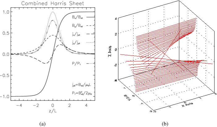
indis-(a) (b)
[image:25.595.150.502.198.627.2](c)
tinguishable. There is noycomponent of the magnetic field and the current density is completely
perpendicular to the magnetic field. For this equilibrium it is the plasma pressure gradient that
maintains the force balance, with the maximum plasma pressure at the centre of the sheet.
The Harris Sheet with Constant Guide Field
A constant guide magnetic field in theydirection can be added to the Harris sheet without altering the structure of the equilibrium. This guide field introduces a field aligned current but it is
impor-tant to remember that the current density is completely independent of the strength of the guide
magnetic field added. So adding a guide field to introduce a field aligned current is not the same as a force-free equilibrium where increasing the shear of the magnetic field increases the current
density in the system. The constant guide field also adds no free energy to the system. Figure
2.1(c)shows a 3D plot of magnetic field lines for a constant guide field ofBy = B0. It can be clearly seen how the constant guide field adds shear and twist to the system.
Linear Force-Free Field
A simple linear force-free field is given by,
Bx = B0sin (αz), (2.17) By = B0cos (αz), (2.18)
B2 = constant (2.19)
jx = αB0
µ0
sin (αz), (2.20)
jy = αB0
µ0
cos (αz), (2.21)
P = PT − B02
2µ0
=constant. (2.22)
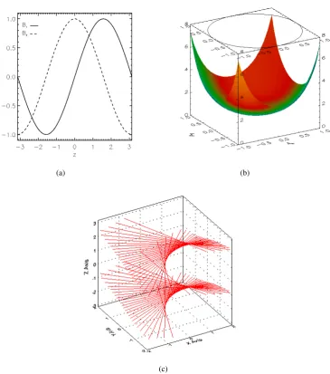
The profiles of the magnetic field components and current density components are shown in Figure
2.2(a)and a 3D plot of magnetic field lines is shown in Figure2.2(b)whereα= 1.0. The magnetic fields are periodic and the pressure is constant. The current density is completely aligned with the
(a) (b)
Figure 2.2: 1D plots of the profiles of the magnetic field components and current density compo-nents for a linear force-free current sheet (2.2(a)) combined with a 3D plot of magnetic field lines alongzpassing throughx= 0,y= 0(2.2(b)).
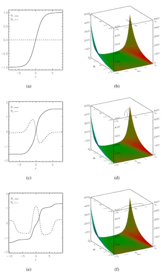
The Force-Free Harris Sheet
In contrast to the Harris sheet there is the force-free Harris sheet. This is a 1D non-linear force-free equilibrium where,
Bx = B0tanh
z
L
, (2.23)
By =
B0
cosh Lz, (2.24)
B2 = constant (2.25)
jx = B0 µ0L
tanh Lz
cosh Lz, (2.26)
jy = B0 µ0L
1
cosh2 Lz, (2.27)
P = PT − B02
2µ0
=constant. (2.28)
The profiles of the magnetic field components and current density components with a 3D plot of
magnetic field lines are shown in Figure2.3. There is in this case a spatially varying symmetricy component of the magnetic field which is non-zero at the centre of the current sheet. The magnetic
pressure is constant. It is theycomponent of the magnetic field, rather than the plasma pressure,
(a) (b)
Figure 2.3: 1D plots of the profiles of the magnetic field components and current density com-ponents for the force-free Harris Sheet (2.3(a)) combined with a 3D plot of magnetic field lines alongzpassing throughx= 0,y= 0(2.3(b)).
Increasing the shear of the field also increases the free energy in the system.
The Combined Harris Sheet
It is also possible to consider the equilbria in between these two extremes where the force balance
is maintained by a balance between theycomponent of the magnetic field and the plasma pressure
where,
Bx = Bx0tanh
z
L
, (2.29)
By =
p
Bx20−2µ0P0
cosh Lz =
By0
cosh Lz, (2.30)
P = P0
cosh2 Lz =
Bx20−By20
2µ0
1
cosh2 Lz, (2.31)
jx = By0 µ0L
tanh Lz
cosh Lz, (2.32)
jy = Bx0 µ0L
1
cosh2 Lz (2.33)
2µ0PT = Bx20, (2.34)
B2x0
2µ0
These types of equilibria will have current densities which are neither completely perpendicular,
nor completely aligned with the magnetic field. They will exhibit some of the properties of both
the Harris sheet and the force-free Harris sheet, depending on for example the strength of the imposed shear field. A simple example is shown in Figure2.4 which shows the profiles of the magnetic field components, current density components and the pressure in Figure2.4(a)and a 3D plot of magnetic field in Figure2.4(b). In this example the ratio of the the maximum value of Byto the maximum value ofBxhas been set toBy0/Bx0 = 1/
√
5and the maximum value of the plasma pressure corresponds to4/5of the total pressure in the system (P0 = 4/5PT).
[image:29.595.152.503.277.483.2](a) (b)
Figure 2.4: 1D plots of the profiles of the magnetic field components, current density components and pressure for the combined Harris Sheet (2.4(a)) combined with a 3D plot of magnetic field lines alongzpassing throughx= 0,y= 0(2.4(b)).
2.2
Multi-Fluid Theory
In the Sec. 2.1.1important 1D MHD equilibria were described. These examples gave insight in to some of the basic properties of different types of equilibria. It is highlighted, for example
that a force-free equilibrium must have a field aligned current and that the field will be highly
sheared and twisted, with the force balance being maintained by the magnetic pressure due to the shear field and not the plasma pressure gradient. The opposite of this is for example the Harris
sheet (Harris 1962), where the force balance is maintained by the plasma pressure gradient and the current density is completely perpendicular to the magnetic field. The main aim of this work was
starting from a pure pressure gradient balanced equilibrium, for example the Harris sheet (Harris 1962), could be compared to simulations starting from a completely force-free equilibrium, for example the force-free Harris sheet. The motivation to study multi-fluid theory is that it treats each particle species as a separate fluid. This means that although it is still not as complex as the
full kinetic theory it does already allow us to gain insight into the bulk properties of each particle
species. This information is useful in identifying key properties that will be needed when trying to find Vlasov-Maxwell equilibria.
2.2.1 Multi-Fluid Equilibrium Equations
Consider the static states of the collisionless multi-fluid equations (∂/∂t = 0). The primary equations that must be solved are,
∇ ·(nsus) = 0, (2.36)
msns[(us· ∇)us] = nsqs[E+us×B]− ∇Ps, (2.37)
µ0j = ∇ ×B, (2.38)
∇ ·B = 0, (2.39)
where the assumption of isotropic pressure has been made. These equations are the continuity equation, the momentum equation, Amp`ere’s law and the solenoidal condition. The electric field
can also be written as the gradient of a scalar functionφwhere,
E=−∇φ. (2.40)
2.2.2 1D Equilibria
Assuming that all quantities depend only on thez coordinate and that the magnetic field can be derived from a vector potentialA. The components of the magnetic field can then be written as
Bx = − dAy
dz , (2.41)
By = dAx
dz . (2.42)
It is also assumed that the bulk velocities for each particle species only have components in thex
andydirections,
By making this assumption the continuity equation, Eq. (2.36) is automatically satisfied asuzs=
0, i.e. d
dz(nsuzs) = 0. (2.44) Also the LHS of the momentum equation, Eq. (2.37) reduces to zero. Hence the primary equation that must be solved is the momentum balance for each species,
nsqs[E+us×B]− ∇Ps=0. (2.45)
The electric field only has azcomponent,
E=−dφ
dzez. (2.46)
The magnetic field is determined by Amp`ere’s law,
∇ ×B = µ0j (2.47)
= µ0
X
s
nsqsus. (2.48)
It must be assumed thatns andPs are related by an appropriate equation of state which can be used later to determine the separate species quantities. To determine the equilibria, a sum of the
momentum equation over all species is carried out. Assuming quasineutrality,
X
s
nsqs= 0, (2.49)
the electric field can be eliminated. Summing the momentum equation over all species results in,
E X
s nsqs
!
+ X
s
nsqsus
!
×B−X
s
∇Ps =0, (2.50)
and using quasineutrality the electric field is eliminated and the equation that is left to be solved
is,
j×B=∇P = dP
dzez, (2.51)
where the total plasma pressure is defined as
P =X
s
There is no field line curvature so this is just the condition that the sum of the magnetic pressure
and plasma pressure across the sheet must be equal to a constant,
B2
2µ0
+P =PT =a constant. (2.53)
The above equations show that the equilibrium solutions are exactly the same as those in MHD. This includes the Harris sheet (Harris 1962) and the force-free Harris sheet. For a detailed de-scription of these equilibria refer back to Sec.2.1.1.
Two-Fluid Case
The advantage of multi-fluid theory is that information about the separate species quantities can
be gained. In this section, the bulk properties for each particle species for the 1D equilibria are discussed where a two-fluid picture is assumed for simplicity. An equation of state for each fluid
is given by,
Ps=kBTsns, (2.54)
whereTsis the temperature of each particle speciessand is assumed to be constant. Assuming
quasineutrality and a two component plasma where,qi =−qe=e, P =kBn
X
s
Ts. (2.55)
This implies the total pressure and the number density have the same profile,
P α n. (2.56)
Also, due to quasineutrality,
Ps=kBTsn, (2.57)
which implies that each species has the same pressure profile as the total pressure,
Psα P. (2.58)
The bulk velocities can also be calculated in this case. The equation for the current density gives
one equation,
j=nX
s
Without loss of generality (in line with MHD), the overall bulk velocity of the fluid is set to zero.
This gives the added condition,
X
s
msus=0. (2.60)
For just two species this is sufficient to calculateus as there are 4 equations and 4 unknowns.
Performing this calculation, the Harris sheet drift velocities are constant for each species and are
only in theydirection where,
uxi = uxe= 0, (2.61)
uyi = − meuye
mi
= B0
en0µ0L me me+mi
=a constant. (2.62)
In the case of the force-free Harris sheet there is a spatially varying drift velocity for each species
in thexandydirections,
uxi = − meuxe
mi
= 1
eµ0n0L me
(me+mi) Bx
cosh(Lz), (2.63)
uyi = − meuye
mi
= 1
eµ0n0L
me
(me+mi) By
cosh(Lz). (2.64)
Finally the electric field can be calculated. Multiplying the equation of motion byms and sum-ming over all species, the electric field is written as,
E=
P
s mqss∇Ps
nP
sms
. (2.65)
It is concluded thatE = 0 in the force-free case as the pressure for each species,Ps, must be equal to a constant. As a final remark, the equation of motion only determines the component of
usperpendicular toB. The parallel component will remain free apart from the constraint provided
by the parallel component ofj. The important properties to note are that, in the case of the Harris sheet, it is the spatially varying number density that maintains the force balance. The particle
density for each species is a maximum at the centre of the current sheet and drops away to zero
as you move away from the centre. There is a constant average drift velocity in theydirection for each species which gives rise to the perpendicular current densityjy. In the force-free case the
force balance is maintained by a spatially varying drift velocity for each species in both thexand ydirections. The particles drift faster at the centre of the sheet than far away from the centre. It is
these differences that are important when considering an investigation to find analogous equilibria
2.3
Summary
In this chapter an overview of important MHD equilibria has been presented. One of the aims
of this work is to investigate 1D Vlasov-Maxwell which are analogous to 1D MHD equilibria, to determine general conditions for force-free VM equilibria and in particular to find distribution
functions that have the force-free Harris sheet as a solution of the steady state Vlasov-Maxwell equations. Therefore in this chapter the general properties of 1D MHD equilibria and some
impor-tant cases have been discussed, as preparation for the discussion of 1D VM equilibria in Chapter
3.
Two examples of force-free fields are shown. A periodic linear force-free field and the non-linear
force-free Harris sheet. In both cases in comparison to the Harris sheet the force-free solutions
have highly sheared magnetic fields. In the force-free cases the force balance is always maintained by the shear magnetic field and the pressure is constant. In the opposite Harris sheet case the
cur-rent density is completely perpendicular to the magnetic field and there is no shearing of the field.
The force balance is maintained by the plasma pressure gradient across the sheet. A combined Harris sheet case is also shown where the force balance is maintained by a balance between the
shear field and the plasma pressure gradient. In this case the magnetic fields are sheared but the
shear is not as great as in the force-free case. The combined Harris sheet case shows that as you make the transition from the anti-parallel Harris sheet through to the force-free Harris sheet the
magnetic fields become more sheared and there is a trade off between the plasma pressure and the
shear field in the force-balance equation.
Multi-fluid equilibria have also been considered. Multi-fluid theory treats each particle species
as a separate fluid and therefore gives an insight in to the bulk particle properties. Firstly it was shown that, assuming a quasineutral plasma and an isotropic pressure that the overall equilibria
are identical to the MHD cases. The Harris sheet, combined Harris sheet and the force-free Harris
sheet are all solutions of the multi-fluid equations.
In particular the two fluid case was considered whereqi = −qe = eand assuming an ideal equation of state and constant temperatures it was shown that the pressure profile for each species
will be proportional to the quasineutral number density. Making the assumption that the overall fluid is at rest which is equivalent to the MHD case where there is no bulk velocity the average drift
velocities for each particle species for the Harris sheet and force-free Harris sheet were found. In
the Harris sheet case there is a constant drift in theydirection consistent with the current density being completely perpendicular to the magnetic field. In the force-free Harris sheet case there
is an average drift of each particle species in thex and y directions which is spatially varying
and aligned with the magnetic field, which is consistent with the definition of a force-free field. Knowledge of the average drift velocites for each particle species are important as it shows that
there must be a large number density at the centre of the current sheet which drops off to zero
far away from the current sheet that maintains the force balance across the sheet. In the opposite
case of the force-free Harris sheet case the particles drift in a direction aligned with the magnetic field and they drift faster at the centre of the current sheet and slower far away. It is the spatially
varying drift velocity that maintains the force balance. Therefore a distribution function which can
describe a force-free solution must give rise to a constant number density and spatially varying average drift velocities for each particle species. It will now be shown how this can be achieved
Vlasov Equilibrium Theory
Parts of the work in this chapter can be found inHarrison and Neukirch(2009b) andHarrison and Neukirch(2009a).
3.1
Introduction
Plasma equilibria are suitable starting points for investigations of, for example, plasma
instabili-ties and plasma waves. In Chap.2, 1D fluid equilibria have been mentioned including single fluid MHD and also collisionless multi-fluid theory with the assumption of isotropic pressure. For colli-sionless plasmas though, the most relevant equilibria are self-consistent solutions of the stationary
Vlasov-Maxwell (VM) equations, (see e.g.Krall and Trivelpiece 1973;Schindler 2007).
This chapter focuses exclusively on non-relativistic one-dimensional quasi-neutral VM equilibria with translational symmetry, with the distribution functions depending only on the Hamiltonian
and the two canonical momenta corresponding to the invariant directions (here chosen to be the x- andy-directions). A large amount of work on translationally invariant 1D VM equilibria of
this kind has been done before (e.g.Tonks 1959;Grad 1961;Harris 1962;Bertotti 1963;Hurley 1963;Nicholson 1963;Sestero 1964,1966;Sestero and Zannetti 1967;Lam 1967;Parker 1967;
Lerche 1967;Davies 1968,1969;Alpers 1969;Su and Sonnerup 1971;Kan 1972;Channell 1976;
Lemaire and Burlaga 1976;Roth 1976;Mynick et al. 1979;Lee and Kan 1979b,a;Greene 1993;
Roth et al. 1996;Attico and Pegoraro 1999;Mottez 2003, 2004;Fu and Hau 2005;Yoon et al. 2006), especially on one-dimensional current sheets and plasma boundary layers, which are of fundamental importance for the structure and stability of plasmas as many plasma activity
pro-cesses, especially magnetic reconnection, (see e.gBiskamp 2000;Priest and Forbes 2000) happen there preferentially.
The aim of this work is not only to add to the solutions of 1D VM that already exist, but to use
some generic properties of the 1D VM equilibrium problem to investigate the conditions for the
existence of force-free 1D VM equilibria (see e.g.Tassi et al. 2008) and to find a VM equivalent of the force-free Harris sheet. An obvious property of 1D VM equilibria is that the structure needs to
be in force balance. In the quasi-neutral case this means that the sum of the magnetic pressure and
one of the diagonal components of the pressure tensor has to be constant. The relevant component of the pressure tensor is the one for the single spatial coordinate upon which the equilibria depend.
Thezcoordinate is chosen, so the component of the pressure tensor in the force balance equation
will bePzz. In a number of papers it has also been noticed that the translationally invariant 1D VM problem is equivalent to the motion of a pseudo-particle in a conservative pseudo-potential
and/or that the force balance for the 1D VM structure is equivalent to pseudo-energy conservation (see e.g.Grad 1961;Sestero 1966;Lam 1967;Parker 1967;Lerche 1967;Alpers 1969;Su and Sonnerup 1971;Kan 1972;Channell 1976;Mynick et al. 1979; Lee and Kan 1979b,a;Greene 1993; Attico and Pegoraro 1999); the pseudo-particle analogy has also recently been used for MHD equilibria inTassi et al.(2008).
Directly connected to the pseudo-particle analogy and the related pseudo-energy conservation law
(equivalent to force balance of the 1D VM equilbrium) is the special role played by Pzz. As was first noticed by Grad (Grad 1961) for the case of vanishing electric potential and only one non-vanishing magnetic field and vector potential component, but otherwise arbitrary distribution
functions, the derivative ofPzz with respect to the non-vanishing component of the vector poten-tial equals (modulo constants) the current density. This was generalized by Bertotti (Bertotti 1963) who included a non-vanishing electric potential and showed that the partial derivative ofPzz with
respect to the electric potential is proportional to the charge density (see alsoSchindler et al. 1973;
Schindler 2007, for the same conclusion for 2D VM equilibria). Lerche (Lerche 1967) then gener-alized this to equilibria with two magnetic field, vector potential and current density components,
but for a restricted class of distribution functions. Channell (Channell 1976) investigated the case of vanishing electric potential and a special class of distribution functions for which he showed
that the two components of the current density are, again modulo constant factors, given by the
partial derivatives of the particle density with respect to the components of the vector potential. If investigated carefully one can see that the full expressions including the constant factors are
again the partial derivatives ofPzz with respect to the components of the vector potential. Using the force balance condition, Mynick et al. (Mynick et al. 1979) then showed that, independently of the distribution function, the partial derivatives ofPzz with respect to the electric potential and
the two components of the vector potential are always proportional to the charge density and the components of the current density, respectively. They also showed that this property is maintained
under the assumption of quasi-neutrality. The authors then use this property to construct 1D VM
case of vanishing electric potential. Similarly to Channell (Channell 1976), they used this prop-erty to construct a number of special distribution functions for 1D VM equilibria. More recently,
Mottez (Mottez 2004) gave a detailed discussion of the role of the full pressure tensor (not just of one component) for distribution functions of the same type as discussed by Channell (Channell 1976), but including the case of non-vanishing electric potential.
The properties ofPzzmake it a very useful quantity to start any investigation of 1D VM equilibria, since all other quantities such as particle density, charge density and current density can be derived
by differentiation.Pzz is also equivalent to the pseudo-potential of the analogous pseudo-particle problem and can thus be used to study the properties of 1D VM equilibria qualitatively without
the need to solve the equilibrium differential equations. In particular, the pseudo-particle analogy
can be used to formulate conditions onPzzthat it has to satisfy to allow the existence of 1D force-free VM equilibria (Tassi et al. 2008). So far only linear force-free 1D VM equilibria are known (Sestero 1967;Bobrova and Syrovatskiˇi 1979;Correa-Restrepo and Pfirsch 1993;Bobrova et al. 2001) and the pseudo-particle analogy can also give some insight into the types of distribution functions permitting a linear force-free solution.
Therefore this chapter is laid out such that in Sec.3.2the basic general theory of quasi-neutral 1D VM equilibria with three constants of motion is presented, rederiving the basic equations given first by Mynick et al. (Mynick et al. 1979) directly from the definitions of the basic quantities. In Sections3.3-3.5several examples of 1D Vlasov-Maxwell equilibria are given which emphasise the usefulness of the properties of Pzz. In Sec. 3.6 general properties of 1D force-free VM equilibria are discussed based on the one-to-one correspondence of the mathematical problem
with the motion of a pseudo-particle in a conservative 2D pseudo-potential. Finally Sec. 3.7and
3.8show how thePzz component of the pressure tensor can be used to determine a distribution function for the force-free Harris sheet and how this can be extended to a complete family of
equilibria that describe the transition between the Harris sheet and the force-free Harris sheet. The
conclusions are presented in Sec.3.9.
3.2
General Theory
It is assumed that all quantities depend only onzand that the magnetic field has componentsBx
and By. The magnetic field components are written in terms of a vector potential
A= (Ax, Ay, Az)where, Bx = −
dAy
dz , (3.1)
By = dAx
and the electric field is the gradient of an electric potentialφsuch that,
E=−∇φ=−dφ
dzez. (3.3)
In this case B and E automatically satisfy the homogeneous steady state Maxwell equations
∇ ·B= 0and∇ ×E=0.
Due to the symmetries of the system (time independence and spatial independence ofxandy) the three obvious constants of motion for each particle species are the Hamiltonian or particle energy
for each speciess,
Hs=
1 2ms(v
2
x+vy2+v2z) +qsφ, (3.4)
the canonical momentum in thexdirection,pxs,
pxs =msvx+qsAx, (3.5)
and the canonical momentum in theydirection,pys,
pys=msvy +qsAy, (3.6)
wheremsandqsare the mass and charge of each species. All positive functionsfssatisfying the
appropriate conditions for existence of the velocity moments and depending only on the constants
of motion,
fs=fs(Hs, pxs, pys), (3.7)
solve the steady-state Vlasov equation,
v·∂fs
∂r +
qs ms
(E+v×B)·∂fs
∂v = 0. (3.8)
To calculate the 1D Vlasov-Maxwell equilibria the remaining inhomogeneous steady-state Maxwell equations,∇ ·E=σ/0and∇ ×B=µ0jmust be solved. These equations reduce to,
−d
2φ
dz2 =
1
0
σ(Ax, Ay, φ), (3.9)
−d
2A x
dz2 = µ0jx(Ax, Ay, φ), (3.10)
−d
2A y
dz2 = µ0jy(Ax, Ay, φ), (3.11)
the following way,
σ(Ax, Ay, φ) =
X s qs Z ∞ −∞ fs
msv2
2 +qsφ, msvx+qsAx, msvy+qsAy
d3v,
(3.12)
jx(Ax, Ay, φ) =
X
s qs
Z ∞
−∞
vxfs
msv2
2 +qsφ, msvx+qsAx, msvy+qsAy
d3v,
(3.13)
jy(Ax, Ay, φ) =
X
s qs
Z ∞
−∞
vyfs
msv2
2 +qsφ, msvx+qsAx, msvy+qsAy
d3v.
(3.14)
Here, the dependence of the charge and current densities on the electric and vector potentials has
been made visible explicitly. Independent of the choice of distribution functionfs, it can be shown (see appendix A) that the charge and current density components always satisfy the equations,
∂σ ∂Ax
+∂jx
∂φ = 0, (3.15)
∂σ ∂Ay
+∂jy
∂φ = 0, (3.16)
∂jx ∂Ay
− ∂jy
∂Ax
= 0. (3.17)
These equations are completely analogous to the relation derived by Schindler and co-workers
(Schindler et al. 1973;Schindler 2007) for the case of distribution functions depending only on the Hamiltonian and a single canonical momentum. Equations (3.15) - (3.17) imply the existence of a potentialP (Schindler 2007), wherePis given by,
P(Ax, Ay, φ) =
X
s
Z ∞
−∞
msvz2fsd3v, (3.18)
which is identified as thePzz component of the pressure tensor. The Eqs. (3.15) - (3.17) are necessary conditions for the force balance of the Vlasov-Maxwell equilibria, which has been
emphasized before by many authors for special cases (see e.g.Grad 1961;Hurley 1963; Lam 1967;Parker 1967;Lerche 1967;Alpers 1969;Su and Sonnerup 1971;Kan 1972;Channell 1976;
Lemaire and Burlaga 1976; Roth 1976;Lee and Kan 1979b,a;Greene 1993;Roth et al. 1996;
Attico and Pegoraro 1999); the sum of the plasma pressure and magnetic pressure must be equal to a constant. The charge density,σ, and the current densities, jx and jy, are given by partial derivatives of the pressure tensor with respect to the electric potential,φand the components of
the vector potential,AxandAy, in the following way (see Appendix A for details):
σ = −∂P
jx = ∂P ∂Ax
, (3.20)
jy = ∂P ∂Ay
. (3.21)
They highlight the important relations between the current density components and thePzz
com-ponent of the pressure tensor. Throughout this work a quasineutral plasma consisting of two
species (electrons and ions) of opposite charge (|qs|=e) will always be assumed. Quasineutrality can be assumed as long as all length scales are much larger than the Debye length. Quasineutrality
does not generally imply that the electric field vanishes (Schindler 2007;Schindler and Birn 2002;
Neukirch 1993).
Quasineutrality corresponds to (3.9) being replaced by
σ(Ax, Ay, φ) =− ∂P
∂φ = 0. (3.22)
This in general can then be inverted to give the quasineutral electric potentialφqnwhere,
φqn=φqn(Ax, Ay). (3.23)
The potentialP is then replaced by its quasineutral versionPqn, wherePqn is a function only of AxandAy,
Pqn(Ax, Ay) =P(Ax, Ay, φqn(Ax, Ay)). (3.24) It should be noted that due to Eq. (3.22),
∂Pqn ∂Ax Ay = ∂P ∂Ax
Ay,φ
+ ∂φqn ∂Ax Ay ∂P ∂φ
Ax,Ay
=
∂P ∂Ax
Ay,φ
, (3.25)
where it is understood that on the right hand sideP is evaluated using the quasineutral electric potential and the subscripts indicate explicitly which quantities are being kept constant during the
differentiation. An analogous equation holds for the derivative ofPqnwith respect toAy. Thus in
Eqs. (3.20) and (3.21) the derivatives ofPcan be replaced by derivatives ofPqnin the quasineutral case. Using Eqs. (3.20) and (3.21) Amp`ere’s law can be written as,
−d
2A x
dz2 = µ0 ∂Pqn ∂Ax , (3.26) −d 2A y
dz2 = µ0 ∂Pqn
∂Ay
. (3.27)
The resulting Vlasov-Maxwell equilibria can now be found by solving these two coupled second