H
I
-MaNGA: H
I
follow-up for the MaNGA survey
Karen L. Masters ,
1,2‹David V. Stark,
3Zachary J. Pace ,
4Frederika Phipps,
2,5Wiphu Rujopakarn,
3,6,7Nattida Samanso,
6Emily Harrington,
1,8Jos´e
R. S´anchez-Gallego,
9Vladimir Avila-Reese,
10Matthew Bershady,
4,11Brian Cherinka,
12Catherine E. Fielder,
13Daniel Finnegan,
1,14Rogemar A. Riffel ,
15,16Kate Rowlands ,
12Shoaib Shamsi,
1Lucy Newnham ,
1,2Anne-Marie Weijmans
17and Catherine A. Witherspoon
41Department of Physics and Astronomy, Haverford College, 370 Lancaster Avenue, Haverford, PA 19041, USA 2Institute of Cosmology and Gravitation, University of Portsmouth, Dennis Sciama Building, Portsmouth PO1 3FX, UK
3Kavli Institute for the Physics and Mathematics of the Universe (WPI), The University of Tokyo Institutes for Advanced Study, The University of Tokyo,
Kashiwa, Chiba 277-8583, Japan
4Department of Astronomy, University of Wisconsin-Madison, 475 N. Charter St., Madison, WI 53726, USA 5School of Physics and Astronomy, University of Southampton, Southampton SO17 1BJ, UK
6Department of Physics, Faculty of Science, Chulalongkorn University, 254 Phayathai Road, Pathumwan, Bangkok 10330, Thailand 7National Astronomical Research Institute of Thailand, Don Kaeo, Mae Rim, Chiang Mai 50180, Thailand
8Department of Physics, Bryn Mawr College, 101 N Merion Ave, Bryn Mawr, PA 19010, USA 9Department of Astronomy, Box 351580, University of Washington, Seattle, WA 98195, USA
10Instituto de Astronom´ıa, Universidad Nacional Aut´onoma de M´exico, A.P. 70-264, 04510 M´exico, D.F., Mexico 11South African Astronomical Observatory, P.O. Box 9, Observatory 7935, Cape Town, South Africa
12Department of Physics and Astronomy, Johns Hopkins University, 3400 N. Charles St., Baltimore, MD 21218, USA 13PITT PACC, Department of Physics and Astronomy, University of Pittsburgh, Pittsburgh, PA 15260, USA 14Department of Physics, Siena College, 515 Loudon Road, Loudonville, NY 12211, USA
15Departamento de F´ısica, CCNE, Universidade Federal de Santa Maria, 97105-900 Santa Maria, RS, Brazil 16Laborat´orio Interinstitucional de e-Astronomia, 77 Rua General Jos´e Cristino, Rio de Janeiro 20921-400, Brazil 17School of Physics and Astronomy, University of St Andrews, North Haugh, St Andrews, KY16 9SS, UK
Accepted 2019 July 7. Received 2019 July 7; in original form 2018 November 11
A B S T R A C T
We present the HI-MaNGA programme of HIfollow-up for the Mapping Nearby Galaxies at Apache Point Observatory (MaNGA) survey. MaNGA, which is part of the Fourth phase of the Sloan Digital Sky Surveys, is in the process of obtaining integral field unit spectroscopy for a sample of∼10 000 nearby galaxies. We give an overview of the HI21cm radio follow-up observing plans and progress and present data for the first 331 galaxies observed in the 2016 observing season at the Robert C. Bryd Green Bank Telescope. We also provide a cross-match of the current MaNGA (DR15) sample with publicly available HI data from the Arecibo Legacy Fast Arecibo L-band Feed Array survey. The addition of HIdata to the MaNGA data set will strengthen the survey’s ability to address several of its key science goals that relate to the gas content of galaxies, while also increasing the legacy of this survey for all extragalactic science.
Key words: catalogues – surveys – galaxies: ISM – radio lines: galaxies.
1 I N T R O D U C T I O N
MaNGA (Mapping Nearby Galaxies at Apache Point Observatory; Bundy et al.2015) is part of the SDSS-IV (Fourth phase of Sloan Digital Sky Survey) programme of surveys (Blanton et al.2017)
E-mail:klmasters@haverford.edu
which began in 2014 and is running until 2020. MaNGA modified the SDSS-III Baryon Oscillation Spectroscopic Survey (BOSS) fibre fed spectrograph (Smee et al.2013) on the Sloan Foundation 2.5-m telescope (Gunn et al.2006) to create pluggable integral field units (IFUs) which group between 19–127 fibres in a hexagonal pattern (or ‘bundle’) across the face of each MaNGA galaxy (Law et al. 2015), ranging in size from 12 to 32 arcsec in diameter. This allows the survey to obtain spatially resolved spectra for a
2019 The Author(s)
large sample of galaxies. The MaNGA instrument has 17 such fibre bundles in each SDSS plate (a sky area with a diameter of 3◦).
MaNGA is observing ∼1600 galaxies per year for a planned sample of∼10 000 galaxies over its full 6 yr duration (Law et al. 2015; Wake et al.2017). In the most recent public release (Data Release 15, or DR15, Abolfathi et al. 2018) MaNGA data for 4621 unique galaxies were made available to the community. These data already make MaNGA the largest IFU survey in the world (e.g. ATLAS-3D, Calar Alto Legacy Integral Field Area Survey (CALIFA) or Sydney AASO Multiobject Integral Field Spectrograph (SAMI) haveN=260, 600, and∼3000 respectively, Cappellari et al.2011; S´anchez et al.2012; Bryant et al.2015), allowing the internal kinematics and spatially resolved properties of stellar populations and ionized gas to be studied as a function of local environment and halo mass across all types of galaxies.
MaNGA will provide the most comprehensive census of the stellar (and ionized gas) content of local galaxies to-date, but galaxies are not made of stars alone. The science goals of MaNGA are focused on understanding the physical mechanisms which drive the evolution of the galaxy population. These goals have been developed into the four key science questions of MaNGA (Bundy et al.2015), all of which crucially depend on understanding not only the stellar content but also the cold gas budget of galaxies in the MaNGA sample. In the next section, we summarize how knowledge of HIcontent contributes to all of MaNGA’s key science questions.
1.1 How HIwill contribute to MaNGA key science questions
(i)How does gas accretion drive the growth of galaxies? Infor-mation on the total cold gas content is a necessary first step to fully explore the role of gas accretion, by revealing the global HIcontent of each galaxy, and in particular galaxies found to have more HI than is typical may be used to reveal gas accretion. Asymmetry in the HIprofile may also correlate with accretion (e.g. Bournaud et al.2005). Finally, knowledge of total content will also provide targets for spatially resolved HIfollow-up to reveal the details of gas accretion.
(ii) What are the relative roles of stellar accretion, major merg-ers, and instabilities in forming galactic bulges and ellipticals?
The cold gas content drives the dynamics of secular evolution (e.g. bars, Athanassoula2003), as dynamically cold gas is a more efficient transport of angular momentum than the stars. Modelling of the shape of the HIprofile, combined with MaNGAs stellar and ionized gas velocity maps may allow us to statistically probe HI distributions – e.g. looking for central holes. This is a technique we plan to investigate in future work. Extended HIis also a better probe of interactions than stellar morphology (e.g. Holwerda et al. 2011).
(iii)What quenches star formation? What external forces affect star formation in groups and clusters?Information about the cold gas content is crucial for understanding the physical mechanisms that regulate gas accretions and quench galaxy growth via the conversion of gas into stars (e.g. see Rosario et al. 2018, who look at the links between active galactic nucleus feedback and CO content). HI-MaNGA data can be combined with CO follow-up to add information on the molecular hydrogen (e.g. ongoing CO follow-up surveys like MASCOT1and JINGLE, Saintonge et al.
1http://www.eso.org/∼dwylezal/mascot
20182) in order to complete this picture across a representative subset of the MaNGA sample. The efficiency of converting atomic into molecular hydrogen, given by the H2-to-HI mass ratio, is tightly related to the large-scale star formation in galaxies (e.g. Leroy et al. 2008). Exploring the dependencies of this ratio on mass, mass surface density, galaxy type, specific star formation rate (SFR), and environment will help to clarify the role of global disc instabilities versus local processes of the interstellar medium in the star formation efficiency of galaxies (e.g. Blitz & Rosolowsky2006; Krumholz, McKee & Tumlinson2009; Obreschkow & Rawlings 2009). These can also be compared with the star formation histories (either from stellar population synthesis, or using current SFR via ionized gas) as well as metallicities obtained the MaNGA data, adding crucial information for this analysis.
(iv)How was angular momentum distributed among baryonic and non-baryonic components as the galaxy formed, and how do various mass components assemble and influence one another?
Without the full baryonic mass accounting for both stars and gas this question cannot be answered. Nowadays, the stellar-to-halo mass relation is one of the most used relations in extragalactic astronomy (Wechsler & Tinker 2018). A generalization of it to the gaseous and total baryonic contents provides relevant informa-tion for understanding the galaxy–halo connecinforma-tion and the main physical processes that drive galaxy evolution. Volume weights can be applied to the MaNGA survey to produce a volume-limited sample (e.g. Wake et al. 2017), in such a way that the galaxy– halo connection for stellar, HI, H2, and baryonic masses will be possible. The baryonic Tully–Fisher relation (e.g. McGaugh et al. 2000; Stark, McGaugh & Swaters2009; Avila-Reese et al.2008) provides the most direct observational link between baryonic mass and dark halo mass. Molecular gas typically does not contribute significantly to the total baryonic mass (MH2∼0.1 M; e.g. Boselli
et al.2014), but HImass can be a significant fraction, or even the dominant component, in the mass range of the MaNGA sample and so the total HImass must be directly measured. Further, MaNGA traces the stellar and ionized gas kinematics out to only 1.5 or 2.5re (Law et al. 2015). HIkinematics (rotation widths) will provide an anchor point for the rotation speed of galaxies in their outer parts.
In this paper, we introduce HI-MaNGA, a program of HI (21-cm line) follow-up of MaNGA galaxies aimed at contributing HI information to help MaNGA data be used to address its key science questions. This first HI-MaNGA paper is intended to introduce the survey and document the first release of data, which was released as a Value Added Catalogue (VAC) in SDSS-IV DR15 (Abolfathi et al. 2018). We provide in this release data from our first year of observing at the Robert C. Byrd Green Bank Telescope (GBT; under project code AGBT16A 095). This comprises the results of observations of 331 MaNGA galaxies. Observations have to-date been completed at GBT for a further∼2000 MaNGA targets; those data will be released in the future.
The structure of this paper is as follows. We describe the target selection for HI-MaNGA and existing HIin Section 2. Our observational strategy and data reduction process is described in Section 3. We show some overview results based on the HIcontent or dynamics of MaNGA galaxies in Section 4, and conclude with a summary in Section 5.
2http://www.star.ucl.ac.uk/JINGLE/
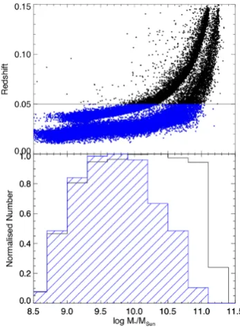
Figure 1. We show the impact that a redshift limit ofcz<15 000 km s−1 which we apply to the HI-MaNGA follow-up programme has on the mass distribution of MaNGA targets. The upper panel shows the redshift–stellar mass distribution of all possible MaNGA targets (upper concentration of points shows the primary sample, lower the secondary). Indicated with the horizontal line is the redshift limit for HI-MaNGA. The lower panel shows the mass distribution for the full MaNGA (unfilled; showing roughly flat mass distribution forM=109–11M) and HI-MaNGA target galaxies (blue hatched; basically MaNGA targets withcz<15 000 km s−1).
2 TA R G E T S E L E C T I O N A N D E X I S T I N G HI
The basic selection for HI-MaNGA targets is all MaNGA observed galaxies withcz<15 000 km s−1, and not obviously in the sky area observed by ALFALFA (Arecibo Legacy Fast Arecibo L-band Feed Array, Haynes et al.2011,2018).3
Our GBT observations (see Section 3) are designed to reach comparablermsnoise to the ALFALFA survey (around 1.5 mJy at 10 km s−1velocity resolution, Haynes et al.2011); the upper redshift limit is chosen partly by the redshift range of ALFALFA, and partly by the distance at our expected depth where we expect more non-detections than non-detections. This redshift cut partially acts as a stellar mass limit in the MaNGA sample because of the way MaNGA is selected (Wake et al.2017). We illustrate this in Fig.1which shows the stellar mass redshift relation (upper) and the mass distribution (lower) of MaNGA and HI-MaNGA targets, respectively. Notice how MaNGA has a flat mass distribution acrossM∼109−11M,
while HI-MaNGA targets are more strongly peaked at M ∼
109.8M
, while basically all low-mass MaNGA galaxies will be followed up in HI, higher mass galaxies are preferentially further away, and therefore less likely to be part of the follow-up presented here. By observing all MaNGA galaxies regardless of morphology we will provide an unbiased (or at least agnostic to morphological properties) census of the HIcontent and the impact this has on galaxy properties.
3There is some deliberate overlap to check cross-calibration. Also, as the final ALFALFA100 catalogue was not released at the start of HI-MaNGA there is some unintentional overlap at the edges of the surveys.
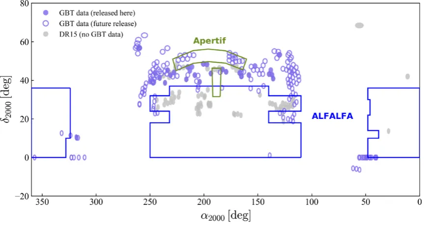
At the beginning of planning for HI-MaNGA, the MaNGA sample that was available was the ‘MPL-4’ list (‘MaNGA Product Launch-4’, an internal name for the subset of MaNGA observations which was then later released in DR13; Albareti et al.2017). This means that all galaxies with HI measurements released in this preliminary data release are part of the DR13 (and therefore also DR15 and later) MaNGA samples. From within this list observing was completed in an order which maximized efficiency on sky, with a secondary goal of finishing HIobservations for MaNGA galaxies on SDSS plates that were partially completed in earlier GBT observing sessions. We show in Fig.2the sky distribution of MaNGA targets, observations, and HIfollow-up (as well as other relevant HIsurveys).
As part of more recent planning for the HI-MaNGA observing, we also performed a cross-match of the MaNGA MPL-7 sample (the set which was released in DR15) with the final ALFALFA (100 per cent) release (Haynes et al.2018). This provides all strong detections (roughly signal-to-noise ratio, S/N>4.5) in ALFALFA. We also extract upper limits for non-detections by measuring the noise at the sky and redshift position of each MaNGA galaxy directly from the cubes. We find a total of 908 of the MaNGA DR15 sample atz <0.05 in ALFALFA (334 detections and 574 upper limits).4
3 G B T O B S E RVAT I O N S A N D DATA R E D U C T I O N
In this paper, we present observations from the first 331 HI-MaNGA targets, using 192.5 h of GBT telescope time (or 35 min telescope time per galaxy). This was completed during the 2016A and 2016B observing semesters (all under proposal code AGBT16A 95).
3.1 Observations
Observations were performed using the L-band (1.15-1.73 GHz) receiver on GBT, which has a full width at half-maximum beam of 8.8 arcmin at these frequencies. We made use of the VErsatile GBT Astronomical Spectrometer (VEGAS) backend.5VEGAS was tuned to place 21cm (1420.405 MHz) emission at the known optical redshift of the MaNGA galaxy (from the NASA Sloan Atlas, Blanton et al.2011) at the centre of the bandpass, which was set to have a width of 23.44 MHz. A total of 4096 channels were used to collect data (which therefore had a raw spectral resolution of 5.72 kHz; or 1.2 km s−1). As this is much smaller than needed to resolve the velocity structure of a typical galaxy, we boxcar smooth by a factor of four (to a resolution of 22.89 kHz, or∼5.0 km s−1) during the final data processing, and then performed a Hanning Smoothing for a final effective velocity resolution of 10 km s−1.6
Observations were done in position switch mode using multiples of 5 min ON/OFF pairs (i.e.∼10 min telescope time). Data were collected in 10 s ‘data samples’ in order to mitigate the impact of time dependent radio frequency interference (RFI) causing catastrophic loss of entire samples (or more usually several samples in a row). In most cases each target was observed for a total of three
4Details of how to access this catalogue can be found athttps://www.sdss.org /dr15/data access/value-added-catalogs/?vac id=hi-manga-data-release-1 5For details on VEGAS, seehttp://www.gb.nrao.edu/vegas/report/URSI201 1.pdf
6As galaxies in our sample range fromz=0.01 to 0.05, the exact value varies by about 5 per cent across the redshift range
Figure 2. The sky distribution of MaNGA observations and HI-MaNGA follow-up. The MaNGA DR15 sample is shown plotted as plates: in grey where there is no GBT data; open purple symbols where data have been taken, but not yet reduced; and filled purple circles show the sky positions of data released here. We also indicate the approximate footprint of the final ALFALFA survey (Haynes et al.2018) in blue and the planned Apertif medium deep survey.
Figure 3. We show thermsnoise as a function of integration time for our observing. The gathering of points atT=900 s reveals our typical integration time around the targeted noise of 1.5 mJy. The solid line indicates at−1/2
relationship for 1.5 mJy in 900 s.
ON/OFF pairs; sometimes, where a strong detection was found early observing this was cut short, and in some cases where significant interference from passing global positioning system (GPS) satellites ruined a significant fraction of ‘samples’ in an ON/OFF pair, an additional set (or sometimes more than one) was obtained. This procedure can be identified in Fig.3which shows the measured
rmsnoise as a function of total integration time in seconds. The vertical strip att=900 s represents observations comprising three sets of 5 min (or 300 s) ON/OFF pairs, while a large number of observations which lost small fractions of time to GPS or other interference scatter below or sometimes above this.
Fig.3also illustrates that our goal to obtain roughly rms=1.5 mJy observations has been largely achieved; where the noise is significantly higher this is typically because the galaxy was a strong HIemitter (and therefore detected even in a noisier spectrum). The
solid line shows a behaviour oft−1/2normalized to 1.5 mJy att= 900 s.
3.2 Data reduction
Data was reduced making use of the customGBTIDL7interface to IDL(the Interactive Data Language8). Data segments free of GPS or other significant interference are first combined, edges trimmed, and narrow-frequency RFI removed before smoothing to the final 10 km s−1resolution.
Calibration was performed using the GBT gain curves which are reported to be highly accurate atLband for simple ON/OFF observing.9Finally, baselines are fit to the signal free part of the spectrum.
The reduced and baseline-fitted spectra for the first 331 targets observed at GBT on this programme are provided as a VAC in SDSS DR15 (Abolfathi et al.2018) accessible on the SDSS Science Archive Server (SAS10); a detailed data model is provided.11 For each observation, we provide a row in an overview catalogue file,12 which also has a data model available.13ThismangaHIallfile includes information on either the detection or non-detection as well as meta data to aid in using in combination with MaNGA data. This is intended to be the structure for future larger data releases
7http://gbtidl.nrao.edu/
8https://www.harrisgeospatial.com/SoftwareTechnology/IDL.aspx 9A flux scale accuracy of 10–20 per cent is reported in the GBTIDL Calibration Document athttp://wwwlocal.gb.nrao.edu/GBT/DA/gbtidl/gbt idl calibration.pdf
10https://data.sdss.org/sas/mangawork/manga/HI/v1 0 1/spectra/GBT16 A 095/
11https://internal.sdss.org/dr15/datamodel/files/MANGA HI/HIPVER/spe
ctra/HIPROP/mangaHI.html
12https://data.sdss.org/sas/dr15/manga/HI/v1 0 1/mangaHIall.fits 13https://internal.sdss.org/dr15/datamodel/files/MANGA HI/HIPVER/m angaHIall.html
[image:4.595.63.271.343.508.2]from the same program, which will have their own corresponding updated data models.
It is also possible to access HI-MaNGA data using the Marvin interface (Cherinka et al.2018).14
3.2.1 Characterizing detections
As all galaxies are observed at their known optical redshift, we determine detection at a fixed smoothing scale by eye. This procedure is standard for similar single-dish surveys; a more quantitative/automated detection scheme is being considered for future HI-MaNGA data releases.
We report the peak S/N calculated as S/N=Sp/rms. This will introduce a slight bias due to the measuredSpbeing elevated by positive noise peaks. The user may prefer to re-calculate S/Nc
= (Sp − rms)/rms from tabulated values. The integrated S/N is more appropriate to assess the significance of detections, and can be calculated as S/Nint=FHI/FHI, error, whereFHI, erroris described below.
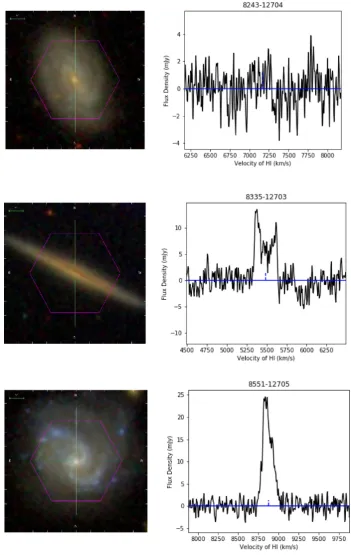
Example detections across low, median, and high S/N are shown in Fig.4. HIwidths like these are characterized using the same procedure as was described in Masters et al. (2014); based on Springob et al. (2005) this is also similar to the measurements per-formed by ALFALFA (Haynes et al.2018). Not all measurements are possible on the lowest S/N detections; which should always be used with caution as errors on extracted quantities will be large, and the likelihood of spurious detections is high.
A summary of all measurements which are provided for each detection (where possible) is given in Table1. We refer the reader to Masters et al. (2014) and references therein for full details of these measurements, but provide here for convenience the formula used to calculate:
(i) The statistical error on the HIflux:
FHI,error=rms
√
vW , (1)
wherev = 10 km s−1is the channel resolution (after Hanning smoothing), andWshould be the width of the profile (ideally the full width of baseline where signal is integrated, a value of 1.2WP20 can be used to approximate this).
(ii) HImasses from fluxes:
MHI/M=2.356×105
D
Mpc
2
FHI Jy km s−1
. (2)
We highlight that we provide raw widths and fluxes (and HI masses) in the catalogue. Users may wish to apply the following corrections to reconstruct more physically representative values:
(i) To correct HImasses for HIself-absorption you may like to use
MHI,c=cMHI, (3)
wherec=(a/b)0.12has been recommended (using the optical axial ratio (a/b), see Giovanelli et al.1994for details).
(ii) To correct HIwidths for inclination effects, cosmological broadening, and the impact of turbulent motions and instrumental resolution use
Wc=
W−2vλ
1+z −t
1
sini, (4)
14For details on this see the tutorial athttps://sdss-marvin.readthedocs.io/e n/stable/tools/catalogues.html#value-added-catalogs-vacs
withv =5.00 km s−1(the effective resolution before Hanning smoothing) and whereλis a factor which accounts for the impact of noise on the effective resolution, taken from the simulations of Springob et al. (2005).15The correctiont=6.5 km s−1is proposed to correct for turbulent motions, (also from the work of Springob et al.2005) and the inclination ican be calculated for a disc of intrinsic thickness,qfrom its observed axial ratio (a/b) using
cosi=
(b/a)2−q2
1−q2 , (5)
and whereq=0.2 is a reasonable average estimate for discs (see Masters et al.2014, and references therein).
(iii) Cosmological corrections are small in this redshift range (0.01< z <0.05), however we list some here (and point the reader to Meyer et al.2017for a full discussion). We re-iterate that these corrections have not been applied in our DR1 catalogue.
(a) The use of Jy km s−1as units of flux (which is standard in HIsurveys in the local Universe) introduces a (1+z)2term into the flux when expressed in units with the dimensions of flux (Jy Hz). This will propagate into all measurements using integrated flux (i.e. HImasses).
(b) Peculiar velocities can introduce significant distance errors in the local Universe (e.g. as explored in Masters, Haynes & Giovanelli 2004). However the minimum redshift limit of the MaNGA survey (z > 0.01) means the impact of this is
<10 per cent on HI-MaNGA masses.
(c) Widths are provided in rest frame. Equation (4) includes the (1 + z) correction which should be applied to correct to observed frame.
3.2.2 Characterizing non-detections
Non-detections are reported just as thermsnoise across the spectrum (in mJy), but we also report a conservative estimate of the HImass upper limit, assuming width ofW=200 km s−1to allow to calculate an estimate of the HIflux which could have remained undetected (to 1σ) as:
FHI,lim<200 rms mJy km s−1, (6)
and therefore the HIupper limit as
MHI,lim/M<2.356×105
D
Mpc
2
FHI,lim Jy km s−1
, (7)
assumingD = vopt/70 km s−1 Mpc−1 (where vopt is the optical redshift of the MaNGA galaxies in the NSA). To be used for statistical analysis, this simple estimate should be corrected so it does not depend on the channel width of the observations (which is implicit in the measurement of therms). A better choice of a 3σ
upper limit (which we do not provide in this catalogue release, but which can be calculated from the information given) would be
FHI,lim=3 rms
√
W vmJy km s−1, (8)
where v = 10km s−1 is the velocity resolution (after Hanning smoothing), and W is the assumed width (e.g. 200 km s−1 as used above, or this could be based on the optically measured rotation from MaNGA). Although channel size, v, is included
15We use the values forv <5 km s−1ofλ=0.005 for log (S/N)<0.6,λ
= −0.4685+0.785log (S/N) for 0.6<log (S/N)<1.1 andλ=0.395 for log (S/N)>1.1.
Figure 4. Example spectra for three MaNGA galaxies with low (i.e. use with caution as it could be not real), average, and high S/N in the HIdetection (peak S/N values are 2.4, 7.5, and 17, while integrated S/N using the flux error in equation (1) are 2.9, 21, and 46 respectively). At the right is shown the baseline subtracted radio spectrum centred on the optical redshift of the galaxy (dashed line) whose SDSSgriimage is shown at left. The galaxies are (from top to bottom) MaNGAID=1-47291, 1-252072, and 1-247382. The MaNGA bundle is indicated by the purple hexagon; recall that the GBT beam atLband is at least 18 times larger than this (8.8 arcmin compared to a maximum bundle size of 32.5 arcsec).
in equation (8), this calculated upper limit will not scale with channel size, as any increase/decrease in channel size will be cancelled by a decrease/increase inrms(which should be calculated at v resolution). On average we find that equation (8) gives
an upper limit ∼1.5 times smaller than that we report in the catalogue (which can therefore be considered a more conservative upper limit) and should be more appropriate in terms of noise statistics.
Table 1. Summary of measurements made on HIdetections.
Name Units Description
Sp mJy The peak HIflux density
S/N – The peak signal tormsnoise ratio
FHI Jy km s−1 The integrated HIflux. Note this is not self-absorption corrected
log (MHI/M) – log of the HImass (in solar masses) from equation (2) assumingD=vopt/70 km s−1Mpc−1 and using the raw HIflux (no correction for self-absorption)
VHI km s−1 Central redshift of the HIdetection (using optical definition for redshift, and in the Barycentric frame)
WM50 km s−1 Width of the HIline measured at 50 per cent of the median (which is also the mean) of the two peaks
WP50 km s−1 Width of the HIline measured at 50 per cent of the peak
WP20 km s−1 Width of the HIline measured at 20 per cent of the peak
W2P50 km s−1 Width of the HIline measured at 50 per cent of the peak on either side
WF50 km s−1 Width of the HIline measured at 50 per cent of the peak−rmson fits to the sides of the profile
Pr,Pl mJy The peak HIflux densities in the low and high velocity peaks respectively
[image:7.595.316.536.277.444.2]ar,al mJy Fit parameters inF(v)=a+bvfits to either side of the profile (used in measuringWF50), br,bl mJy/(km s−1) where the zero-point of the velocity axis in the fit is defined as the central velocity of the HI.
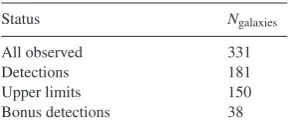
Table 2. Summary of first year of observing for HI-MaNGA at GBT (AGBT16A 95).
Status Ngalaxies
All observed 331
Detections 181
Upper limits 150
Bonus detections 38
4 R E S U LT S
The simplest result we can show is the detection fraction for the programme. This is summarized in Table 2. Out of 331 galaxies observed we report detections consistent with HIcoming from the target galaxy in redshift in 181 cases (i.e. a detection fraction of 55 per cent). We further report 38 ‘bonus’ detections,16 representing HIdetected either at a redshift significantly offset from the target, or in the OFF position. These results should be used with extreme caution as the object emitting the HIis unlikely to be centred in the GBT beam, and therefore beam attenuation may be significant.
For all primary detections (and upper limits for the 150 non-detections), we show the HImass (or limit) plotted against redshift in Fig. 5. The solid line shows our estimated detection limit of 109.4M
at a recessional velocity ofv = 9000 km s−1 (or a distance of 129 Mpc/h70). There is some scatter around this line for observations with significantly higher or lower noise than typical (see Fig.3which shows thermsnoise of all observations).
4.1 HImass fraction
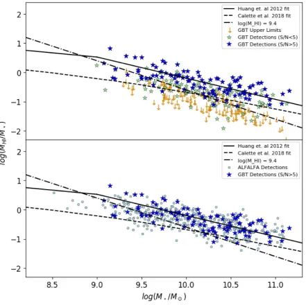
As a check on data quality, we plot in Fig.6our corrected HImass fraction against stellar mass, and compare to results from ALFALFA matches to MaNGA galaxies, as well as the published relations based on all ALFALFA detections from Huang et al. (2012), and the fit to a compilation and homogenization of data from various sources for late-type galaxies in Calette et al. (2018). We use stellar masses from the Pipe3D analysis tool (S´anchez et al. 2016a, b)
16https://data.sdss.org/sas/dr15/manga/HI/v1 0 1/mangaHIbonus.fits
Figure 5. We show the log HImass (uncorrected) versus HIrecessional velocity for all GBT detections and non-detections released in this publica-tion. The grey arrows indicate non-detections with the solid line being the upper limit of HImass for these non-detections. The limit is derived from the inverse square relationship of mass and distance via our median value ofMHI=109.4Mbeing detectable atcz=9000 km s−1.
applied to the MaNGA data and presented in a VAC (S´anchez et al.2018); here we use specifically the MPL-6 version of Pipe3D which used the same set of galaxies as released in DR15, but an earlier reduction pipeline. The HImasses here are corrected for self-absorption following the procedure in Section 3.2.1. Our results follow the published relation (and ALFALFA measurements) well, with some scatter to lower mass fractions, which are mostly low S/N detections, and reflect the survey strategy as a follow-up to optical detections, rather than a blind HIsurvey like ALFALFA, which naturally picks up higher HImass fraction galaxies in a stellar mass selected sample (because galaxies which scatter below the relation will preferentially have low S/N detections which may not be believed in the targeted follow-up but not in a blind survey).
4.2 Star formation and HIdetections
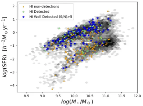
In Fig.7, we show a star formation stellar mass plot for the MaNGA DR15 sample. The integrated SFRs and stellar masses shown in this
[image:7.595.91.237.307.371.2]Figure 6. The corrected HImass fraction (logMHI/M) plotted against Pipe3D stellar masses for MaNGA galaxies. Upper: showing only data from the GBT
observing published here. Lower: GBT strong detections plus ALFALFA data for MaNGA galaxies. The relations found by Huang et al. (2012) and Calette et al. (2018) are overplotted as the solid and dashed lines, respectively, while the dotted–dashed line shows gas fraction for a constant HImass of logMHI/M =9.4.
plot are taken from the Pipe3D analysis of MaNGA data (S´anchez et al.2018). All DR15 galaxies are shown in grey to reveal the typical distribution of MaNGA galaxies on the plot (with star forming galaxies in the upper sequence, and ‘quiescent’ galaxies below. We highlight HInon-detections (red points), weak detections (blue stars; S/N<5 in HI), and strong detections (cyan stars; S/N>5 in HI) from the HIdata released with this publication, which we note does not cover all DR15 MaNGA galaxies (i.e. a grey point means that the galaxy does not have HIdata, not that it does not have HI).
As is expected, HIdetections concentrate in the star-forming sequence of this plot, however we note that detections are found in some quiescent MaNGA galaxies and some star-forming galaxies have no detected HI. This trend has been previously noted in HIsurveys (e.g. Brown et al. 2015; Saintonge et al.2017), who
note that the molecular gas is more strongly correlated to the star formation properties than HI. Further work using this sample will investigate how the HIcontent of MaNGA galaxies correlates with star formation properties in more detail.
5 S U M M A RY A N D C O N C L U S I O N S
In this paper, we introduce the HI-MaNGA follow-up survey of the MaNGA sample (Bundy et al.2015). This programme is aiming to obtain HIfollow-up observations for a large subset of the MaNGA galaxies, selected only on redshift (cz<15 000 km s−1). We present here the observational and data reduction strategy, as well as basic results from the first year of observing at the GBT (under project code AGBT16A 95) which obtained HImeasurements (or upper limits) for 331 MaNGA galaxies. These data are released as a VAC in
Figure 7. Total SFR from the Pipe3D analysis of MaNGA data is plotted against the stellar mass of MaNGA galaxies. The entire DR15 MaNGA sample is shown in the greyscale contours (hexbin log scale with number), while those detected in HIare shown by the blue (S/N<5) or cyan stars (S/N>5), and non-detections are shown as red points. Note that the plotted HIdata covers only a subset of DR15 galaxies. Nevertheless it is clear that while HIdetections concentrate on the star-forming sequence, they are not completely absent in quiescent galaxies.
SDSS DR15 (Abolfathi et al.2018) available to download viahttps: //data.sdss.org/homeand with a catalogue available in CasJobs.17
These data are already in use by the wider MaNGA science team. Published work which has already made use of these GBT HIdata include a study of the properties of quiescent dwarf galaxies (Penny et al.2016), a paper on an unusual galaxy showing evidence for hot ionized gas infall (which is not detected in HIwith GBT; Lin et al.2017a) and a paper which presents Atacama Large Millimeter Array (ALMA) data for a sample of three green valley galaxies (Lin et al.2017b).
We have performed a cross-match of the MaNGA DR15 sample with the ALFALFA100 catalogue. We find 1308 of the MaNGA DR15 galaxies have HIdata in ALFALFA (334 detections, and 574 upper limits). We provide our cross-match as an electronic table.
We show some simple plots using these data in combination with MaNGA measurements (or other ancillary data). These include the HImass fraction as a function of stellar mass, and an illustration of where HIdetections lie on the star-formation–stellar mass plot. These provide an illustration of the kind of science which will be enabled by HIfollow-up for MaNGA.
These data will provide a valuable resource to combine with MaNGA data for studies of galaxy evolution and understanding the role of cold gas content which we will explore in future work. The addition of HIdata to the MaNGA data set will strengthen the survey’s ability to address several of its key science goals that relate to the gas content of galaxies, while also increasing the legacy of this survey for all extragalactic science.
AC K N OW L E D G E M E N T S
The Green Bank Observatory is a facility of the National Science Foundation operated under cooperative agreement by Associated Universities, Inc. We would like to acknowledge the many GBT
17https://skyserver.sdss.org/CasJobs/
operators who helped implement this programme, which was entirely conducted with remote observations.
Funding for the SDSS IV has been provided by the Alfred P. Sloan Foundation, the U.S. Department of Energy Office of Science, and the Participating Institutions. SDSS-IV acknowledges support and resources from the Center for High-Performance Computing at the University of Utah. The SDSS web site iswww.sdss.org.
SDSS-IV is managed by the Astrophysical Research Consor-tium for the Participating Institutions of the SDSS Collabora-tion including the Brazilian ParticipaCollabora-tion Group, the Carnegie Institution for Science, Carnegie Mellon University, the Chilean Participation Group, the French Participation Group, Harvard-Smithsonian Center for Astrophysics, Instituto de Astrof´ısica de Canarias, The Johns Hopkins University, Kavli Institute for the Physics and Mathematics of the Universe (IPMU)/University of Tokyo, Korean Participation Group, Lawrence Berkeley National Laboratory, Leibniz Institut f¨ur Astrophysik Potsdam (AIP), Institut f¨ur Astronomie (MPIA Heidelberg), Max-Planck-Institut f¨ur Astrophysik (MPA Garching), Max-Planck-Max-Planck-Institut f¨ur Extraterrestrische Physik (MPE), National Astronomical Observa-tories of China, New Mexico State University, New York University, University of Notre Dame, Observat´ario Nacional/MCTI, The Ohio State University, Pennsylvania State University, Shanghai Astronomical Observatory, United Kingdom Participation Group, Universidad Nacional Aut´onoma de M´exico, University of Arizona, University of Colorado Boulder, University of Oxford, University of Portsmouth, University of Utah, University of Virginia, University of Washington, University of Wisconsin, Vanderbilt University, and Yale University.
This work makes use of the ALFALFA survey, based on observa-tions made with the Arecibo Observatory. The Arecibo Observatory is operated by SRI International under a cooperative agreement with the National Science Foundation (AST-1100968), and in alliance with Ana G. M´endez-Universidad Metropolitana, and the Universities Space Research Association. We wish to acknowledge all members of the ALFALFA team for their work in making ALFALFA possible, and we also thank Martha Haynes for granting access to ALFALFA cubes to calculate upper limits for all MaNGA galaxies.
This research made use of Marvin, a core PYTHON pack-age and web framework for MaNGA data, developed by Brian Cherinka, Jos´e S´anchez-Gallego, Brett Andrews, and Joel Brown-stein (Cherinka et al.2018).
WR is supported by the Thailand Research Fund/Office of the Higher Education Commission Grant Number MRG6080294 and Chulalongkorn University’s CUniverse.
FP and DF acknowledge Summer Research Funding from the South East Physics Network (www.sepnet.ac.uk) and Keck North-east Astronomy Consortium (KNAC) respectively.
MAB acknowledges NSF Award AST-1517006. KNAC is funded via NSF Award AST-1005024.
We acknowledge the careful reading of the anonymous referee who helped catch many small (and not so small) errors in the first version of this paper.
R E F E R E N C E S
Abolfathi B. et al., 2018,ApJS, 235, 42 Albareti F. D. et al., 2017,ApJS, 233, 25 Athanassoula E., 2003,MNRAS, 341, 1179
Avila-Reese V., Zavala J., Firmani C., Hern´andez-Toledo H. M., 2008,AJ, 136, 1340
Blanton M. R. et al., 2017,AJ, 154, 28
Blanton M. R., Kazin E., Muna D., Weaver B. A., Price-Whelan A., 2011, AJ, 142, 31
Blitz L., Rosolowsky E., 2006,ApJ, 650, 933 Boselli A. et al., 2014,A&A, 570, A69
Bournaud F., Combes F., Jog C. J., Puerari I., 2005,A&A, 438, 507 Brown T., Catinella B., Cortese L., Kilborn V., Haynes M. P., Giovanelli R.,
2015,MNRAS, 452, 2479
Bryant J. J. et al., 2015,MNRAS, 447, 2857 Bundy K. et al., 2015,ApJ, 798, 7
Calette A. R., Avila-Reese V., Rodr´ıguez-Puebla A., Hern´andez-Toledo H., Papastergis E., 2018, Rev. Mex. Astron. Astrofis., 54, 443
Cappellari M. et al., 2011,MNRAS, 413, 813 Cherinka B. et al., 2018, preprint (arXiv)
Giovanelli R., Haynes M. P., Salzer J. J., Wegner G., da Costa L. N., Freudling W., 1994,AJ, 107, 2036
Gunn J. E. et al., 2006,AJ, 131, 2332 Haynes M. P. et al., 2011,AJ, 142, 170 Haynes M. P. et al., 2018,ApJ, 861, 49
Holwerda B. W., Pirzkal N., de Blok W. J. G., Bouchard A., Blyth S.-L., van der Heyden K. J., Elson E. C., 2011, MNRAS, 416, 2401 Huang S., Haynes M. P., Giovanelli R., Brinchmann J., 2012,ApJ, 756, 113 Krumholz M. R., McKee C. F., Tumlinson J., 2009,ApJ, 693, 216 Law D. R. et al., 2015,AJ, 150, 19
Leroy A. K., Walter F., Brinks E., Bigiel F., de Blok W. J. G., Madore B., Thornley M. D., 2008,AJ, 136, 2782
Lin L. et al., 2017a, ApJ, 837, 32
Lin L. et al., 2017b, ApJ, 851, 18
Masters K. L., Haynes M. P., Giovanelli R., 2004,ApJ, 607, L115 Masters K. L., Crook A., Hong T., Jarrett T. H., Koribalski B. S., Macri L.,
Springob C. M., Staveley-Smith L., 2014,MNRAS, 443, 1044 McGaugh S. S., Schombert J. M., Bothun G. D., de Blok W. J. G., 2000,
ApJ, 533, L99
Meyer M., Robotham A., Obreschkow D., Westmeier T., Duffy A. R., Staveley-Smith L., 2017,PASA, 34, e052
Obreschkow D., Rawlings S., 2009,MNRAS, 394, 1857 Penny S. J. et al., 2016,MNRAS, 462, 3955
Rosario D. J. et al., 2018,MNRAS, 473, 5658 Saintonge A. et al., 2017,ApJS, 233, 22 Saintonge A. et al., 2018,MNRAS, 481, 3497 S´anchez S. F. et al., 2012,A&A, 538, A8
S´anchez S. F. et al., 2016a, Rev. Mex. Astron. Astrofis., 52, 21 S´anchez S. F. et al., 2016b, Rev. Mex. Astron. Astrofis., 52, 171 S´anchez S. F. et al., 2018, Rev. Mex. Astron. Astrofis., 54, 217 Smee S. A. et al., 2013,AJ, 146, 32
Springob C. M., Haynes M. P., Giovanelli R., Kent B. R., 2005,ApJS, 160, 149
Stark D. V., McGaugh S. S., Swaters R. A., 2009,AJ, 138, 392 Wake D. A. et al., 2017,AJ, 154, 86
Wechsler R. H., Tinker J. L., 2018,ARA&A, 56, 435
This paper has been typeset from a TEX/LATEX file prepared by the author.