A Robust and Effective Method for Solving Two Point BVP in Modelling Viscoelastic Flows

(1)

https://www.scirp.org/journal/am ISSN Online: 2152-7393

ISSN Print: 2152-7385

DOI: 10.4236/am.2020.111003 Jan. 7, 2020 23 Applied Mathematics

A Robust and Effective Method for Solving

Two-Point BVP in Modelling Viscoelastic Flows

Mohamed El-Gamel, Ola Mohamed, Neveen El-Shamy

Department of Mathematical Sciences, Faculty of Engineering, Mansoura University, Mansoura, Egypt

Abstract

Chebyshev collocation method is used to approximate solutions of two-point BVP arising in modelling viscoelastic flow. The scheme is tested on four non-linear problems. The comparison with other methods is made. The results demonstrate the reliability and efficiency of the algorithm developed.

Keywords

Chebyshev, Collocation, Viscoelastic Flow, Fifth-Order, Nonlinear

1. Introduction

In modelling viscoelastic flows, differential equations of elliptic-hyperbolic op-erator types arise. Simulations of such flows have been studied extensively lately. The main characteristics of such elliptic-hyperbolic operators can be captured in a nonlinear fifth order two-point boundary value problem in one dimension [1] [2]. The elasticity parameter in the problem is of major importance in the inves-tigation; that is, if it is increased, then depending on the formulation of the problem.

Many researchers have discussed solutions of viscoelastic flow model, like the Galerkin method discussed in [1], collocation method discussed in [2], the Rung- Kutta discussed in [3], the homotopy method discussed in [4]. Hermitian finite elements in [5] and the shooting method in [6] [7] [8]. Some authors have dis-cussed other methods of solution of this model in [9] [10] [11].

In this paper, we are going to introduce Chebyshev-collocation method for the numerical solution of the fifth-order non-linear two-point boundary value prob-lem in modelling viscoelastic flow:

( )

4

d d d 1 1

1 ,

d d d 2 2

y y

f x x

x x x

ε

 ₊  ₌ _{− ≤ ≤}  

  (1)

How to cite this paper: El-Gamel, M., Mohamed, O. and El-Shamy, N. (2020) A Robust and Effective Method for Solving Two-Point BVP in Modelling Viscoelastic Flows. Applied Mathematics, 11, 23-34.

https://doi.org/10.4236/am.2020.111003

Received: November 18, 2019 Accepted: January 4, 2020 Published: January 7, 2020

(2)

DOI: 10.4236/am.2020.111003 24 Applied Mathematics concerned to the posterior boundary conditions

2

1 d 1

0

2 d 2

d 1

at 0.

2 d

y y

x

y

c

x ε

_± ₌ _± ₌        

₋ ₌ _>  

 

(2)

with regard to the given positive constants ε and c which act as elasticity pa-rameter and a boundary stress, respectively. Moreover, c is equal unity in this paper.

In recent years, a lot of attention has been devoted to the study of Chebyshev methods to investigate various scientific models. Using these methods made it possible to solve Troeschs problem [12], twelfth-order boundary-value problems [13], high-order nonlinear ordinary differential equations [14], linear integro- differential equations [15], fourth-order Sturm-Liouville problems [16], Genera-lized Sturm-Liouville problems [17], the parabolic inverse problem [18], two- dimensional heat equation [19], fractional diffusion equation [20], elliptic partial differential equations [21], integral and integro-differential equations of the third kind [22], the constant mobility Cahn-Hilliard equation in a square domain [23], Lane-Emden problem [24]. Recently, has been made numerical comparison of sinc-collocation and Chebychev-collocation methods for determining the eigen-values of Sturm-Liouville problems with parameter-dependent boundary condi-tions by El-Gamel [25].

Chebyshev methods for ordinary differential equations have many salient fea-tures due to the properties of the basis functions and the manner in which the problem is discretized. The approximating discrete system depends only on pa-rameters of the differential equation. There are many advantages of using Che-byshev polynomials as expansion function presented in that are good represen-tations of smooth functions. What we do here is to seek a special Chebyshev so-lution which also satisfies the given boundary conditions.

We organize our paper as follows. In Section 2, we present the preliminaries which we used in this paper. Method of the solution is given in Section 3. Some numerical results are presented in Section 4 to show the efficiency of the pro-posed method. Finally, we draw some conclusions and closing remarks.

2. Essential Relations

Chebyshev polynomial formula of the first kind of degree m is chiefly defined and bounded in interval

[

−1,1

]

see [26]

( )

(

1

( )

)

[ ]

cos cos , cos , 0,

m

T x = m − x x=

φ φ

∈ π

or, in didactic organism,

(

cos

)

cos

( )

, 0,1, ,

[

1,1

]

m

T φ = mφ m=  x∈ −

As for the shifted Chebyshev polynomial T∗

( )

x of the first kind on interval

[ ]

a b, .

( )

2

, .

2

m m

a b

T x T q q x

b a

∗ ₌ ₌  ₋ + 

(3)

DOI: 10.4236/am.2020.111003 25 Applied Mathematics With leading coefficient is equal to ₂ 1 2

m m

b a

−  

 ₋ 

  , by Compensation in the previous equation

( )

2

. 2

m m

a b

T x T x

b a

∗ ₌   ₋ + 

 _{− } 



 

In addition, the definition of the collocation points is worded as follow

cos , 0,1, , .

2 i

b a a b i

x i N

b a N

−  +   π 

= __ _+ _ __ =

−

   

   (3)

Moreover, the relation between Chebyshev coefficient matrix A and A∗( )k in the interval

[ ]

a b, is

( )k 4 k k

b a

∗   ∗

= _ ₋ _

A M A

where

0 1

, , ,

2 N

a

a a

τ

∗

∗_{= } ∗ ∗



 

A 

T =T∗ result from the characteristics of Chebyshev polynomial. All in all, the use of half interval 1 1

2 x 2

− ≤ ≤ _{is more favored in modelling} viscoelastic flows. The shifted Chebyshev polynomials can also be worded as follows

( )

(

1

( )

)

2 cos cos 2 .

m m

T∗ x =T x = m − x

This is deduced from definition of the collocation points: 1

cos , 0,1, , .

2 i

i

x i N

N   π 

= _ _ __ =

 

   (4) Similarly, the relation between Chebyshev coefficient matrix A and A∗( )k in the interval 1 1,

2 2

₋      is

( )

4 , 0,1, ,5.

k k k

k

∗ ₌ ∗ ₌

A M A 

3. Method of Solution

Let is assume the approximate solution y x

( )

of the main problem (1) and its derivatives is

( )

0

, 0.5 0.5

N r r r

y x a T∗ ∗ x x

=

∑

− ≤ ≤ ₍₅₎

( )

_{( )}

( )

_{( )}

0

, 0,1, 2, , 5.

N _k k

r r r

y x a∗ T∗ x k

=

∑

=  (6)

(4)

DOI: 10.4236/am.2020.111003 26 Applied Mathematics are

( )

_{( )}

( )

_{( )}

4 . k

k k k

y x x

y x x x

∗ ∗ ∗ ∗ ∗ ∗ =       = =   T A

T A T M A (7) whereas the definitions of ultimate matrices are:

( )

_{( )}

( )

_{( )}

( )

_{( )}

( )

0 0 0

1 _, ( ) 1 _, 1

k k k k N N N y x

y x T x

y x y x T x

y x _y _x T x

    _ _     _ _       =_ _ =_ _ =_ _               _ _  

Y Y T

  

and

( 1) ( 1)

1 3

0 0 0 2

2 2

0 0 2 0 1 0

0 0 0 3 0

0 0 0 0 0

0 0 0 0 0 0 _N _N

N N N N + × +       −     =             M             (8)

for odd N.

( 1) ( 1)

1 3 1

0 0 0

2 2 2

0 0 2 0 0

0 0 0 3 1 0

0 0 0 0 0

0 0 0 0 0 0 _N _N

N N N N + × + −          ₋  =             M             (9)

for even N. We need the following lemma where  and K are both positive in-teger.

Lemma 1. [13] [14] The following relation holds ( )

_{( )}

( )

_{( )}

( )

_{( )}

( )

_{( )}

( )

_{( )}

( )

_{( )}

( )

_{( )}

( )

_{( )}

( )

_{( )}

( )

_{( )}

( )

_{( )}

( )

_{( )}

( ) ( )

(

)

0 0 0 0

1 1 1 1

* * * * 0 0 0 0 0 0 4 k k k k k k

N N N N

k

k k

y x y x y x y x

+                   =                         = = Y Y

T M A T M A

                  (10) where

( )

0 1 * 0 0 0 0 ,

0 0 _N

(5)

DOI: 10.4236/am.2020.111003 27 Applied Mathematics

*

* *

*

0 0

, and .

0 0

   

   

=_ _ =

 

   

   

 

M A

A M

M A

 

   

 

We need the following the theorem:

Theorem 2. If the considered approximate solution of the problem (1) is (7), so that the discrete Chebyshev system is availed by

,

∗₌

WA F (11) where

(

)

4 4 6 * * 5

4 ∗ ε4 ∗

= +

W T M T M A T M

Proof. Replacing each term of (1) with the approximation defined in (7) and (10), and applying the collocation points (4) to it.

The matrices for the boundary conditions subjected to Equation (2) are

2 2

1 1

4 0,

2 2

1 1

4 0,

2 2

1 4

2 c

∗ ∗

∗

 ₌   ₌

   

   

₋ ₌ ₋  ₌

   

   

₋  ₌

 

 

T T M

T M

(12)

Thus, in the matrix

[

W F;

]

we will replace 5th rows by the Equation (12), we

have the augmented matrix _W F ; _ .

∗₌

WA F (13) Now we will solve a linear system (13) of N+1 equations of the N+1 un-known coefficients ar, r=0,1,,N. So as to gain the coefficients of the ap-proximate solution ∗

A by the Q-R method. Algorithm

• _{Input (integer)}_N_. • _{Input (double)}_tol_.

• _{Input (array)}A_old =A₀ (Initial approximation, A0 with N+1 dimension, can be chosen so that the boundary conditions are satisfied).

• W A

(

old

)

Anew=F is a linear algebraic equation system. Then solve this sys-tem to find Anew.

• _If A_old−A_new <tol then A_new =A, break (the program is finished).

• _{Else then} A_old ←A_new.

4. Examples and Comparison

In this section we give an illustrative example to authenticate the obtained results on Equation (1). The performance of Chebyshev method is measured by the root mean square errors Echebyshev which is defined as

( )

2

Chebyshev Exact Chebyshev

0

N

i i

i

E y x y x

=

(6)

DOI: 10.4236/am.2020.111003 28 Applied Mathematics Example 1: [1] [2] [3] Consider the following fifth order nonlinear two-point BVP

4

d d d 1 1

1 12, ,

d d d 2 2

y y

x

x x x

ε

 ₊  ₌ _{− ≤ ≤}

 

 

whose exact solution is

( )

1 2 1 2

.

2 4

y x = _x − _

[image:6.595.210.451.107.185.2]

 

Table 1 exhibits a comparison between the root mean square errors obtained by using the present method, Beam function using Galerkin, Beam function us-ing Collocation, Runge-Kutta methods and Chebyfun for Example 1. This com-parison shows the strength of the first scheme. Figure 1 demonstrates Chebyshev approximate solution versus the exact solution.

Example 2: [1] [2] [3] Consider the following fifth order nonlinear two-point BVP

4

2 2

4

d d d 1 1 1 1

1 120 600 , ,

d d d 4 20 2 2

y y

x x x x

x x x

ε ε

 ₊  _{= −} ₊  ₋  ₋  _{− ≤ ≤}   

 

    

( )

2 1 2_.

4 y x = −x x_ − _

[image:6.595.209.539.495.588.2]

 

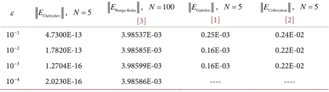
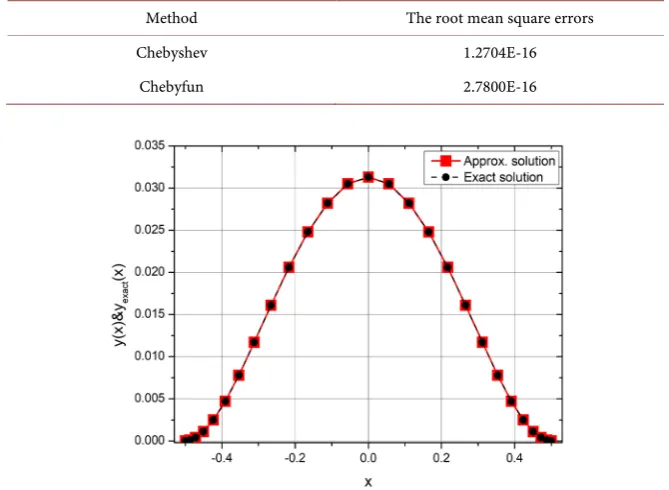
Table 2 represents a comparison between the root mean square errors with the methods in [1] [2] [3]. Table 3 shows a comparison of between the root mean square errors of Chebyshev and Chebyfun at 3

10

ε ₌ − _and 5

N= for Example 2. The graph of Chebyshev approximate solution and the exact solution of have been plotted in Figure 2.

Table 1. Comparison of the root mean square errors at ε=₁₀−1 for Example 1.

Method The root mean square errors

Chebyshev, N=5 1.743E-18

Chebyfun 8.664E-18

Runge-Kutta methods, N=100 [3] 6.899E-03

Beam function using Galerkin, N=4 [1] 0.975E-04

Beam function using Collocation, N=4 [2] 0.855E-03

Table 2. Comparison of the root mean square errors for Example 2, for the present method, Galerkin, collocation methods and Runge-Kutta method.

ε EChebyshev , N=5

Runge-Kutta

E , N=100

[3]

Galerkin

E , N=5 [1]

Collocation

E , N=5

[2]

10−1 _4.7300E-13 _3.98537E-03 _0.25E-03 _0.24E-02

10−2 _1.7820E-13 _3.98585E-03 _0.16E-03 _0.22E-02

10−3 _1.2704E-16 _3.98599E-03 _0.16E-03 _0.22E-02

[image:6.595.209.539.633.725.2]

(7)

[image:7.595.206.541.90.335.2]

Table 3. Comparison of the root mean square errors at 3

10 ε₌ − _and

5

N= for Example 2.

Chebyshev 1.2704E-16

[image:7.595.263.490.376.544.2]

Chebyfun 2.7800E-16

Figure 1. The exact solution and approximation solution for Example 1.

Example 3: [1] [2] [3] Consider the following fifth order nonlinear two-point BVP

( )

4

d d d 1 1

1 , ,

d d d 2 2

y y

f x x

x x x

ε

 ₊  ₌ _{− ≤ ≤}  

 

( )

1 2 1 1

sin .

2 4 2

y x = _x − _ π_x− _

π    

(8)

( )

2 2 2

2

2 2 2 2

2 2

2

2 2 2

1 1 1

12 sin 4 cos

2 4 2 2

1 1 1 1

40 cos 2

8 4 8 2

1 1 1

12 40 sin 2

8 4 2

1 1

5 .

8 4

f x x x x x

x x x

x

ε

π        

= _π _ − _− _ π_ − _− π π_ − _

     

 

 _ _ _ _ _ _

+ π π  −  −  −  π − 

     

 

 

     

+ π _ π _ − _− _ π_ − _

   

 

 _ _ 

+ π π _ − _ + 

 

 

 

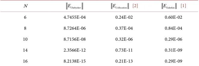
Tables 4-7 illustrate the comparison between result of Chebyshev polynomial method and result of methods in [1] and [2] at 1 3

10 ,10 ,10

ε₌ − − _{and 10}3_with_N

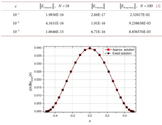
from 6 to 16. Besides, Table 8 depicts ε with values 10−1_{, 10}−2_{and 10}−3_{that has}

[image:8.595.251.500.73.201.2]

an impact on the result of Chebyshev polynomial method at N=18, Chebfun matlab program and the Runge-Kutta in [3] at N =100. Figure 3 demonstrates Chebyshev approximate solution versus the exact solution.

10

ε₌ − _{for Example 3.}

N EChebyshev ECollocation [2] EGalerkin [1]

6 4.3706E-04 0.22E-02 ----

8 1.0349E-05 0.43E-04 0.84E-02

10 1.1865E-07 0.44E-06 0.19E-06

14 3.8885E-12 0.12E-10 0.20E-09

[image:8.595.209.539.333.437.2]

16 1.2817E-14 0.38E-13 0.18E-09

10

ε₌ − _{for Example 3.}

6 4.7455E-04 0.24E-02 0.60E-02

8 8.7264E-06 0.37E-04 0.84E-04

10 8.7156E-08 0.32E-06 0.29E-06

14 2.3566E-12 0.73E-11 0.31E-09

16 8.2138E-15 0.21E-13 0.29E-09

Table 6. Comparison of the root mean square errors at ε=10 for Example 3.

6 0.19E-02 0.95E-02 ----

8 1.1786E-04 0.11E-02 0.27E-04

10 2.3777E-06 0.91E-05 0.16E-06

14 1.9856E-10 0.69E-09 0.13E-10

[image:8.595.209.540.468.579.2]

(9)

[image:9.595.209.541.90.194.2]

10

ε= _{for Example 3.}

6 7.9662E-04 0.40E-02 ----

8 1.5049E-05 0.20E-03 0.14E-03

10 1.8040E-06 0.69E-05 0.16E-06

14 1.1496E-10 0.47E-09 0.13E-10

[image:9.595.207.538.233.488.2]

16 4.9300E-13 0.20E-10 0.13E-10

Table 8. Comparison of the root mean square errors for Chebyshev polynomial method and the Runge-Kutta method for Example 3.

ε EChebyshev , N=18 EChebyfun ERunge-Kutta , N=100 [3]

10−1 _1.9836E-16 _2.84E-17 _2.52017E-02

10−2 _4.1631E-16 _1.01E-16 _9.238658E-03

10−3 _1.0646E-15 _6.71E-16 _8.836376E-03

Example 4: Now we turn to a singular problem

( )

4

4 2

d d d 1 1 1 1

1 , ,

d d d 2 2

y y

y y f x x

x x x x x

ε

 ₊  ₊ _′₊ ₌ _{− ≤ ≤}  

 

and

( )

2 2 3 2 2 2

2 2 2

1 1 1

1440 4 8 6

4 4 4

1

8 720 24,

4

f x x x x x x x

x x x

ε        =   −  +  − +  −       

 

 

 

+ _ − _+ −  

( )

2 2 1 2

2 .

4 y x = x _x − _

 

[image:9.595.210.488.523.706.2]

(10)

( )

4

d d d

1

d d d

y y

p x y d x y b x y f x

x x x

ε

 ₊  ₊ _′′₊ _′₊ ₌  

 

( )

0, 0;

( )

1 , 0;

( )

1 2, 0;

1.5, 0. 0, 0. 0, 0.

x x x x x

p x d x b x

x x x

≠ ≠  ≠

 

= ₌ = ₌ =

=

  

The computational results are summarized in Table 9.

Table 10 exhibits a comparison between the root mean square errors at 1

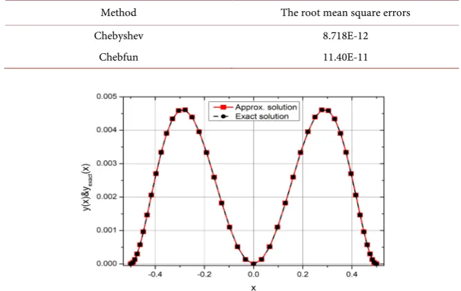
[image:10.595.243.505.74.136.2]

10 ε₌ − and N=6 for Example 4 obtained by using Chebyshev method and Chebfun. Figure 4 demonstrates Chebyshev approximate solution and the exact which ap-pears to be in good agreement with each other.

5. Conclusion

[image:10.595.208.539.397.461.2]

In this article, we present a method to approximate the solution of viscoelastic flows. The numerical method is based on the operational matrix of Chebychev polynomials. We present four examples, the first three examples are nonlinear fifth-order differential equation and fourth example is singular nonlinear. We compared the results of this algorithm with others and showed the accuracy and potential applicability of the given method. The proposed method is a powerful tool for obtaining novel numerical solutions of such equations. It is advisable to use it for other nonlinear differential equations.

Table 9. Comparison of the root mean square errors at N=6 for Example 4.

ε EChebyshev

10−1 _8.7184E-12

10−2 _2.9893E-14

[image:10.595.206.540.493.704.2]

10−3 _9.3948E-15

10 ε₌ − _and

6

N= for Example 4.

Chebyshev 8.718E-12

Chebfun 11.40E-11

(11)

Conflicts of Interest

The authors declare no conflicts of interest regarding the publication of this pa-per.

References

[1] Davies, A., Karageorghis, A. and Phillips, T. (1988) Spectral Galerkin Methods for the Primary Two-Point Boundary Value Problem in Modelling Viscoelastic Flows. International Journal for Numerical Methods in Engineering, 26, 647-662. https://doi.org/10.1002/nme.1620260309

[2] Davies, A., Karageorghis, A. and Phillips, T. (1988) Spectral Collocation Methods for the Primary Two-Point Boundary Value Problem in Modelling Viscoelastic Flows. International Journal for Numerical Methods in Engineering, 26, 805-813. https://doi.org/10.1002/nme.1620260404

[3] Attili, B. (2000) Initial Value Methods for the Primary Two Point Boundary Value Problems in Modelling Viscoelastic Flows. International Journal of Computer Ma-thematics, 74, 379-390. https://doi.org/10.1080/00207160008804949

[4] Syam, M. and Attili, B. (2005) Numerical Solution of Singularly Perturbed Fifth Order Two Point Boundary Value Problem. Applied Mathematics and Computa-tion, 170, 1085-1094. https://doi.org/10.1016/j.amc.2005.01.003

[5] Marchal, J. and Crochet, M. (1986) Hermitian Finite Elements for Calculating Vis-coelastic Flow. Journal of Non-Newtonian Fluid Mechanics, 20, 187-208.

https://doi.org/10.1016/0377-0257(86)80021-0

[6] Attili, S., Elgindi, M. and El-Gebeily, A. (1997) Initial Value Methods for the Eige-nelements of Singular Two Point Boundary Value Problems. AJSE, 22, 67-77. [7] Attili, S. (1993) On the Numerical Implementation of the Shooting Methods to the

One Dimensional Singular Boundary Value Problems. International Journal of Com-puter Mathematics, 47, 65-75. https://doi.org/10.1080/00207169308804163

[8] Elgindi, B. and Langer, W. (1994) On the Shooting Method for a Class of Two Point Singular Nonlinear Boundary Value Problems. International Journal of Computer Mathematics, 51, 107-118. https://doi.org/10.1080/00207169408804270

[9] O’Mally, R. (1974) Introduction to Singular Perturbation. Academic Press, New York. [10] Kevorkian, J. and Cole, J. (1981) Perturbation Methods in Applied Mathematics.

Springer, Berlin.https://doi.org/10.1007/978-1-4757-4213-8

[11] Phillips, T. (1989) On the Potential of Spectral Methods to Solve Problems in Non- Newtonian Fluid Mechanics. Numerical Methods for Partial Differential Equations, 5, 35-43. https://doi.org/10.1002/num.1690050104

[12] El-Gamel, M. and Sameeh, M. (2013) A Chebychev Collocation Method for Solving Troesch’s Problem. International Journal of Mathematics and Computer Applica-tions Research, 3, 23-32.

[13] El-Gamel, M. (2015) Chebychev Polynomial Solutions of Twelfth-Order Boundary- Value Problems. British Journal of Mathematics & Computer Science, 6, 13-23. https://doi.org/10.9734/BJMCS/2015/8874

[14] Akyuz-Dascioglu, A. and Erdik-Yaslan, H. (2011) The Solution of High-Order Nonli-near Ordinary Differential Equations by Chebyshev Series. Applied Mathematics and Computation, 217, 5658-5666. https://doi.org/10.1016/j.amc.2010.12.044

(12)

Mathemat-DOI: 10.4236/am.2020.111003 34 Applied Mathematics ics, 72, 491-507. https://doi.org/10.1080/00207169908804871

[16] El-Gamel, M. and Sameeh, M. (2012) An Efficient Technique for Finding the Eigen-values of Fourth-Order Sturm-Liouville Problems. Applied Mathematics, 3, 920-925. https://doi.org/10.4236/am.2012.38137

[17] El-Gamel, M. and Sameeh, M. (2014) Generalized Sturm-Liouville Problems and Chebychev Collocation Method. British Journal of Mathematics & Computer Science, 4, 1124-1133. https://doi.org/10.9734/BJMCS/2014/7670

[18] Ranjbar, M. and Aghazadeh, M. (2018) Collocation Method Based on Shifted Che-byshev and Radial Basis Functions with Symmetric Variable Shape Parameter for Solving the Parabolic Inverse Problem. Inverse Problems in Science and Engineer-ing, 27, 369-387.https://doi.org/10.1080/17415977.2018.1462355

[19] Gumgum, S., Kurul, E. and Savasaneril, N. (2018) Chebyshev Collocation Method for the Two-Dimensional Heat Equation. CMMA, 3, 1-8.

[20] Agarwal, P. and El-Sayed, A. (2018) Non-Standard Finite Difference and Chebyshev Collocation Methods for Solving Fractional Diffusion Equation. Physica A, 500, 40-49. https://doi.org/10.1016/j.physa.2018.02.014

[21] Ghimire, B., Lamichhane, A., et al. (2020) Hybrid Chebyshev Polynomial Scheme for Solving Elliptic Partial Differential Equations. Journal of Computational and Applied Mathematics, 364, 1123. https://doi.org/10.1016/j.cam.2019.06.040

[22] Sakran, M. (2019) Numerical Solutions of Integral and Integro-Differential Equa-tions Using Chebyshev Polynomials of the Third Kind. Applied Mathematics and Computation, 351, 66-82.https://doi.org/10.1016/j.amc.2019.01.030

[23] Lee, K. (2020) Chebyshev Collocation Method for the Constant Mobility Cahn-Hilliard Equation in a Square Domain. Applied Mathematics and Computation, 370, Article ID: 124931. https://doi.org/10.1016/j.amc.2019.124931

[24] Sharma, B., Kumar, S., Paswan, M. and Mahato, D. (2019) Chebyshev Operational Matrix Method for Lane-Emden Problem. Nonlinear Engineering, 8, 1-9.

https://doi.org/10.1515/nleng-2017-0157

[25] El-Gamel, M. (2014) Numerical Comparison of Sinc-Collocation and Chebychev- Collocation Methods for Determining the Eigenvalues of Sturm-Liouville Problems with Parameter-Dependent Boundary Conditions. SeMA Journal, 66, 29-42. https://doi.org/10.1007/s40324-014-0022-9