Interaction between a surface quasi geostrophic buoyancy anomaly jet and internal vortices

Interaction between a surface quasi-geostrophic buoyancy anomaly jet and internal vortices

J.N. Reinaud,1,a) D.G. Dritschel,1,b) and X. Carton2,c)

1)_{University of St Andrews, Mathematical Institute, North Haugh,}

St Andrews KY169SS, UK

2)_{Laboratoire d’Oc´eanographie Physique et Spatiale, IUEM, UBO/UBL,}

Technopole Brest Iroise, 29280 Plouzane, France

(Dated: 19 July 2017)

This paper addresses the dynamical coupling of the ocean’s surface and the ocean’s interior. In particular, we investigate the dynamics of an oceanic surface jet, and its interaction with vortices at depth. The jet is induced by buoyancy (density) anomalies at the surface. We first focus on the jet alone. The linear stability indicates there are two modes of instability: thesinuousand thevaricosemodes. When a vortex in present below the jet, it interacts with it. The velocity field induced by the vortex perturbs the jet and triggers its destabilisation. The jet also influences the vortex by pushing it under a region of co-operative shear. Strong jets may also partially shear out the vortex. We also investigate the interaction between a surface jet and a vortex dipole in the interior. Again, strong jets may partially shear out the vortex structure. The jet also modifies the trajectory of the dipole. Dipoles travelling towards the jet at shallow incidence angles may be reflected by the jet. Vortices travelling at moderate incidence angles normally cross below the jet. This is related to the displacement of the two vortices of the dipole by the shear induced by the jet. Intense jets may also destabilise early and form streets of billows. These billows can pair with the vortices and separate the dipole.

PACS numbers: 47.20.Ft, 47.32.C, 47.32.Ef, 47.55.Hd

Keywords: Surface quasi-geostrophy, quasi-geostrophy, jets, vortex dynamics

a)_{Electronic mail: jean.reinaud@st-andrews.ac.uk}

b)_{Electronic mail: david.dritschel@st-andrews.ac.uk}

I. INTRODUCTION

Mesoscale vortices play an important part in the transport of momentum, heat and other tracers such as salinity in the oceans. Current estimates1 _{indicate that such vortices may} contribute 50% or more to the overall transport. Modern satellite imagery and measurements provide a good picture of the vortices populating the ocean surface. But vortices exist also at depth. Although many vortices at depth induce a signal at the surface, we do not know the full three-dimensional structure of oceanic vortices in general. Available information has come from limited measurement campaigns at sea2_{, or ARGO float profiles}3_{. However,} these are too sparse to provide any comprehensive description of such vortices. Under these circumstances, numerical modelling may provide helpful insights on how vortices at depth behave and interact with dynamical surface structures such as buoyancy anomalies.

Vortices coexist, and therefore interact, with other vortices or with other dynamical structures such as jets. These jets may develop at depth and are related to distributions of potential vorticity. Alternatively, they can be generated at the surface by either potential vorticity or by anomalies in the density (or buoyancy) field. In the present paper we address the latter situation.

Previous works have focused on a single deep vortex interacting with elliptical patches of surface buoyancy4 _{or with a surface buoyancy filament}5_{. Sokolovskiy et al.}6 _{studied the} interaction between a surface jet and subsurface vortices in a three-layer model. In their study, the jet was generated by the central part of a large gyre. The purpose of this research was to propose a theoretical framework for the study of the interaction of Mediterranean Eddies (Meddies) with the Azores jet and front. The SEMAPHORE campain7–9 (‘Structure des Echanges Mer-Atmosphere, Proprietes des Heterogeneites Oceaniques : Recherche Ex-perimentale’) of 1993-1995 indeed showed the interaction between the Azores jet and one or several Meddies and dipolar structures where a Meddy (anticyclone) also interacted with a cyclone. From these measurements, the vortices diameter is shown to be of the same order of or smaller than the width of the jet. The features have length scales which range from 50km (Meddies) to 130km (Azores jet width) for which the quasi-geostrophic approximation is well suited. Vandermeisch et al.10 _{also studied in a two and a half layer model the interaction}

crossing the Azores Current.

Here we study a similar interaction but in a different context. Instead of generating the jet by a large gyre, we consider a finite-width distribution of surface buoyancy anomaly. This distribution of buoyancy induces a jet at the surface. The influence of the surface jet penetrates downwards but is strongest near the surface. We first describe the characteristics of the jet alone. In particular, we investigate its linear stability and examine its nonlinear evolution when perturbed by an unstable mode. We next investigate the jet when it interacts with vortices at depth. We first consider a single vortex. A single vortex does not move by itself, although it is entrained by the jet when it is in its vicinity. The vortex tends to align with the part of the jet with which it is in co-operative shear. Intense jets are also able to partially shear out the vortex, with adverse shear being more destructive. We next consider a pair of opposite-signed vortices, a vortex dipole, interacting with the jet. A dipole has a self-induced velocity, and has therefore a motion relative to the jet even when it is distant from it. Several scenarios are possible. The dipole can cross below the jet or be reflected by it. Intense jets can separate the dipole, and even partially destroy its component vortices.

The paper is organised as follows. The mathematical model is introduced in section II. The linear stability and the nonlinear dynamics of the jet alone is discussed in section III. The interaction between the surface buoyancy jet and a monopolar vortex is presented in section IV while section V addresses the interaction between the jet and a dipole. Conclusions and ideas for future research are offered in section VI.

II. THE QUASI-GEOSTROPHIC MODEL

The quasi-geostrophic model is the simplest dynamical model which takes into account the dominant effects of the background planetary rotation and the stable density stratification in the ocean. This model is derived from a Rossby number Ro = U/(f L) expansion of the Boussinesq equations, for O(1) Burger number Bu= (Ro/F r)2_{. Here, U is a characteristic} horizontal velocity scale, L is a horizontal length scale, f is the Coriolis frequency, and

F r = U/(N H) is the Froude number, where H is a vertical length scale, and N is the buoyancy (or Brunt-V¨ais¨al¨a) frequency. For the sake of simplicity, we assume that both f

and N are constant. We replace the physical depth z∗ by a stretched vertical coordinate

In the coordinates (x, y, z), the three-dimensional quasi-geostrophic inversion operator, for continuous stratification, is a simply the Laplacian ∆. The linearity of this operator allows one to decompose the total streamfunction of the flowψ into the sum of two terms. The first term ψi is the streamfunction induced by the potential vorticity distribution in the interior of the ocean, while the second part ψs is induced by the surface buoyancy distribution at

z = 0. The inversion equations to be solved are

ψ =ψi+ψs, (1)

∆ψi =q, ∆ψs= 0, (2)

∂ψs ∂z

z=−H

= 0, ∂ψs

∂z z=0 = b

N, (3)

∂ψi ∂z

z=−H

= 0, ∂ψi

∂z z=0

= 0, (4)

where a flat, impermeable ocean bottom at z = −H is assumed. The incompressible hori-zontal velocity u(x, y, z, t) is found from the total streamfunction ψ using

u=∇⊥ψ =

−∂ψ ∂y, ∂ψ ∂x . (5)

Additionally, in the absence of friction and diabatic effects, both the potential vorticity (hereinafter referred to as PV) q and the buoyancyb are materially conserved:

Dq

Dt = 0, and

Db

Dt = 0. (6)

In the last equation, the buoyancy b is only advected at the surface. Finally, we take the horizontal directionsx and y to be periodic, with period 2π without loss of generality. The scales of the vortex structures placed within the domain are taken to be sufficiently small to limit the effects of periodicity.

III. THE JET

A. Geometry

We first investigate the dynamics of the jet alone. In this case, it is simpler to consider

the surface z = 0 itself. The problem is then formally governed by the Surface Quasi-Geostrophic (SQG) equations11_{. Retaining the horizontal periodicity, we consider a surface} buoyancy distribution (at z = 0) of the form

¯

b(y) =   

 

2bm

y a

r 1− y

2

a2 |y| ≤a,

0 |y|> a

(7)

in the fundamental periodic domain −π≤x≤π, −π≤y≤π.

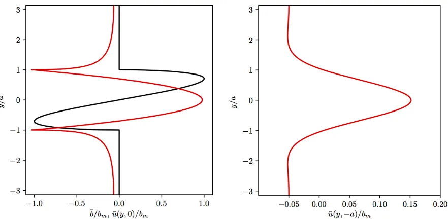
The buoyancy profile ¯b and the resulting longitudinal (along-jet) velocity profile ¯u are shown in Figure 1. The figure also shows the velocity induced at a depth of z = −a to illustrate the effect of the jet in the ocean interior. We see that the jet at depth is wider and smoother than at the surface. This can be explained by the depth-dependence of the horizontal Fourier decomposition of the streamfunction. Sinceψs is harmonic, the horizontal Fourier coefficients of ψs at depth z are ˆψks(z) = ˆψks(z = 0)e

|k|z_{, where k = (k, l) is the} horizontal wavevector (recall that z < 0 is the ocean interior). High wavenumber Fourier modes thus decay more rapidly with depth than low wavenumber ones. Note also that since the profile is x−independent, the y−component of velocity ¯v = ∂ψs/∂x = 0. Hence, the basic flow at the surface can be seen as uni-directional. Note, in Figure 1 u¯ is obtained via a Fourier transform in spectral space asuˆl =−iˆbl, whereuˆl andˆbl are the Fourier coefficients

of the functions u¯(y) and¯b(y), respectively, at a chosen depth z (here 2048 coefficients have been used).

B. Linear stability

We next examine the linear stability of the jet. The stability of jets has been studied extensively, particularly within two-dimensional incompressible flows12,13_{. It is well known} that two distinct branches of instabilities exist for such flows: thesinuous and thevaricose

modes, which are distinguished by the symmetry of their eigenmodes.14 _{The stability of} a surface buoyancy jet has not been addressed within the context of the Surface Quasi-Geostrophic (SQG) model to our knowledge. We expect however, due to similarities in the problems, the jet will likely exhibit both sinuous and varicose modes.

FIG. 1. The surface quasi-geostrophy buoyancy jet considered in this study: Left: non-dimensional buoyancy anomaly profile ¯b(y)/bm (black) and associated non-dimensional longitudinal velocity profile ¯u(y)/bm (red) versus the scaled transversal coordinate y/a at the surface z = 0. Right: ¯

u(y)/bm at a depth of z=−a.

η(x,y, t¯ ). The perturbed buoyancy field at the surface is

b(y) = ¯b(¯y) = ¯b(y−η) = ¯b(y)−ηd

¯_b

dy +O(η

2_{). (8)}

The linearised kinematic condition for the displacement states

∂η ∂t + ¯u

∂η ∂x =v

0

, (9)

where the transverse perturbation velocity v0 can be recovered from the linear buoyancy perturbation b0 = −η d¯b/dy by inversion (i.e. by solving the associated Poisson problem).

As the basic state is independent of x, we may seek perturbations of the form

η(x, y, t) =<{η˜(y)ei(kx−σt)}, (10)

i.e. having a single longitudinal wavenumber k, where σ(k)is the frequency (or growth rate if imaginary). In general, there are a continuum of frequencies and corresponding eigenmodes

˜

transverse velocity is first calculated in spectral space from

ˆ

vk = ikψˆk =

−ik

√

k2_+l2 ˆ

b0_{, with (11)}

ˆ

b0 ₌ Z ∞

−∞

b0e−ily0dy0 = Z a

−a

b0e−ily0dy0. (12)

Taking the inverse Fourier transform in y, we have

v_k0 = 1 2π

Z ∞ −∞

ˆ

vkeilydl, (13)

from which we obtain the following eigen-problem after substitution into (9):

(ku¯(y)−σt)˜η(y) = 2kbm

πa2 Z a

−a ˜

η(y0) 1−2y 02 p

1−(y0_/a)2K0(k|y−y 0_|)

dy0. (14)

Here we have used the identity

Z ∞

−∞

eil(y−y0₎

√

k2_+l2dl = 2K0(k|y−y 0_|)

. (15)

This equation does not appear to have an analytical solution, and hence we solve it numer-ically. To do this, the integral is discretised after the substitution y = −acosθ, θ ∈ [0, π],

over n = 2048 equally spaced intervals in θ. This leads to a 20482 _{algebraic eigenvalue} problem for each value of ka. We determine the eigenvalues (complex frequencies) σ for 0 ≤ ka ≤ 3.3 in increments of ∆(ka) = 0.002. Convergence of the results was checked by comparing with lower resolution calculations. Figure 2 shows the two largest growth rates for the unstable modes σi normalised by the characteristic jet shear bm/a, versus the nor-malised wavenumber ka. We find two continuous, smooth curves σi(k) which cross over at (kc_{a, σ}c

ia/bm) = (0.546,0.081). Each curve corresponds to a different mode of instability. For k < kc (long waves), the dominant mode of instability is varicose. For k > kc this switches to sinuous which remains dominant until both modes stabilise around ka = 3.25 (the short-wave cut-off). This result is in contrast with the well-known stability of the two-dimensional, incompressible Bickley jet for which the sinuous mode is always dominant, and is unstable over a range of wavenumbers twice as large as the range of unstable wavenumbers of the varicose mode14. The basic velocity profile of the Bickley jet is however significantly different from the one considered in this study.

In the present case, the peak instability for the sinuous mode occurs at ka= 1.772 with

σia/bm ' 0.260 while the peak instability for the varicose mode occurs at ka = 1.586 with

FIG. 2. Non-dimensional growth rates of the two modes of instabilityσia/bm existing on a surface quasi-geostrophic jet as a function of normalised wavenumber ka. The sinuous mode is in black while the varicose mode is in red.

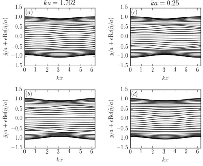
The spatial structure of the two modes of instability is illustrated in Figure 3. We plot a selection of the deformed iso-buoyancy lines y(x,y¯) = ¯y+Re{˜η(¯y)eikx_{} for the two most} unstable modes for ka = 0.25 < kca and ka = 1.762 > kca. The sinuous mode, which is the second fastest growing mode for k < kc_{, and the fastest growing mode for k > k}c _is symmetric (˜η(−y¯) = ˜η(¯y)), while the varicose mode is antisymmetric (˜η(−¯y) = −˜η(¯y)).

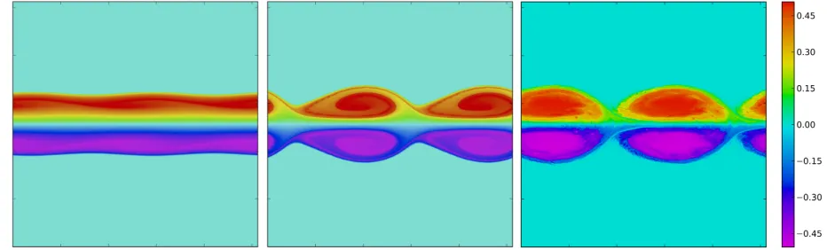
We next illustrate the nonlinear evolution of the jet initially perturbed by a small am-plitude eigenmode using CLAM (the Combined Lagrangian Advection Method)15 adapted to SQG, on a 10242 _{inversion grid. Figure 4 shows the time evolution of the jet perturbed} by the most unstable mode for ka = 1.762 (sinuous) close to the peak instability. To limit the influence of the periodic images in the y−direction, we ensure that the computational domain contains two longitudinal periods. As the maximum buoyancy anomaly is bm = 0.5,

FIG. 3. Deformation of iso-buoyancy contours (eigenmodes) associated with the linear instabilities of a surface quasi-geostrophic jet. (a) Most unstable mode forka= 1.762, (b) second most unstable mode for ka= 1.762, (c) most unstable mode for ka= 0.25, and (d) second most unstable mode forka= 0.25. One every 70 contours are shown from the 2048 iso-buoyancy lines mapping the jet width.

thins; eventually this shear is great enough to cause instability5,16_.

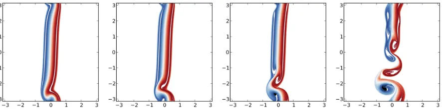
FIG. 4. Time evolution of the buoyancy anomaly for a surface quasi-geostrophic jet perturbed by the most unstable mode (sinuous) with ka = 1.762, and bm = 0.5. Times shown (left to right): t= 20,40, and 97.5.

FIG. 5. Time evolution of the buoyancy anomaly for a surface quasi-geostrophic jet perturbed by the most unstable mode (varicose) with ka= 1.584, and bm0.5. Times shown (left to right): t= 25,50 and 97.5.

As a check on the above analysis, we next compare the nonlinear growth of the instability with the prediction of the linear stability analysis during the early stage of the flow evolution. In the nonlinear results, we compute the perturbation kinetic energy

Kp(t) = 1 2

Z Z

Domain

(u(x, y, t)−u¯(y))2+v(x, y, t)2

dx dy, (16)

which is expected to grow like Kp ∝ e2σit since the integrand is proportional to perturbation

fields squared, to leading order. Figure 6 shows ln(pKp(t)), for both modes of

(dashed). There is good agreement at early times, before the instability saturates. The weaker initial growth is due to the initial perturbation adjusting to the most unstable eigenmode for the symmetry selected.

FIG. 6. Time evolution of ln(pKp), where Kp is the perturbation kinetic energy. The slope of the dashed line gives the growth rate predicted by the linear stability analysis for (a) the sinuous mode atka= 1.762, and (b) the varicose mode at ka= 1.584.

IV. INTERACTION BETWEEN THE JET AND A MONOPOLAR

VORTEX

We next investigate the interaction between a surface jet and a single vortex at depth. For this purpose we use the CASL (Contour Advective Lagrangian) algorithm17_{, adapted} to the three-dimensional quasi-geostrophic model, and including a buoyancy distribution at the surface4. The geometry is illustrated in Figure 7. The depth of the domain is set to

H = 2π so that the model ocean occupies −2π < z < 0. The overall size of the domain is then (2π)3_{. Recall that the vertical coordinateis rescaled by the ratio N/f 1; hence, in} the original physical dimensions, horizontal scales are much larger than vertical scales. The vortex at depth is taken to be a sphere of uniform PV q0, and of diameter d=a, the same as the half-width of the jet. In all simulations, we seta= 0.5. This means thatd/H '0.08. For a 5km-deep ocean, this corresponds to a structure with a vertical span of 400m, a scale comparable with actual observations2_{. This geometry also allows one to confine the jet in} the horizontal and to limit the influence of periodic images.

In this section, the jet is initially parallel to the y−axis. The vortex is located at a depth

hfrom the surface and can be offset in the x-direction from the jet axis by a distance %. An important non-dimensional parameter characterising the interaction is

Λ = bm

aq0 = Tq

Ts

, (17)

which is the ratio of a scale of the shear induced by the jet, bm/a, to the PV of the vortex,

q0. The parameter Λ can also be seen as the ratio of a typical time scale associated with the vortex, Tq, to a time scale associated with the jet, Ts. A large value of Λ corresponds to a strong jet interacting with a relatively weak vortex. We set q0 = 2π without loss of generality and we adapt bm to obtain the targeted value of Λ.

Note that the PV in the vortex is positive, so the vortex rotates in the counter-clockwise direction in all cases. The direction of the jet is set by the sign of bm. For bm > 0, the jet flows in the positive y direction (at its centre), and vice versa. However, since the jet contains both signs of buoyancy anomaly, half of the jet is always in co-operative shear with the vortex (rotating in the same direction), while the other half is in adverse shear. As a consequence, the sign of bm is irrelevant. The two situations bm > 0 and bm < 0 are symmetric. We restrict attention therefore to bm >0 in this study.

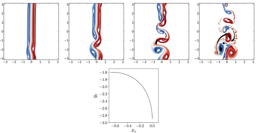
FIG. 8. Surface jet and an internal vortex with h/a = 1, Λ = 1, % = 0. Top panels: top view of the flow at timest= 1,2,3,and 4.4. Jet (blue whereb <0, red whereb >0), vortex (black). The buoyancy contour interval is ∆b=bm/50. Bottom: trajectory of the vortex centre.

flows. Notably, 1024 layers are used to represent the interior PV (where present). Most of these layers have no PV variations and thus require no computational work to evolve the PV distribution. The layers however enable a more accurate representation of the vertical variation of PV and a more accurate inversion to find the velocity field. Interior PV and surface buoyancy contours are followed in a Lagrangian manner (as connected points on curves), and regularised by ‘surgery’18_{at a small scale set to a 16}th _{of the inversion grid size} (corresponding to a resolution of 40963 or finer). This setup is standard in CASL, and can be referred to as a 2563_{-CASL simulation, all the other settings being implied}19_.

Figure 8 illustrates the typical interaction between a vortex and a jet when the vortex is initially located on the jet axis. Here, the vortex is initially placed at (x, y, z) = (0,−π+

since the velocity induced by the jet decreases with depth, the vortex is not advected at the same velocity as the perturbation at the surface. Also, the vortex does not remain aligned with the jet axis. The vortex is displaced towards the part of the jet in co-operative shear. This is confirmed by tracking the vortex centre xc=

RRR

V xdV / RRR

V dV in time, where V is the volume of the uniform PV vortex. The internal vortex tends to align with the nearest counter-clockwise billow forming at the surface. This is similar to the vortex alignment observed for like-signed vortices.20 The vortex also feels the more destructive influence of the adverse shear induced by the right-hand side of the jet. A part of the vortex is sheared out and is stretched into a filament as the flow evolves.

FIG. 9. Top view of a surface jet and an internal vortex withh/a= 1, att= 4.4 (same as bottom right frame in Figure 8) for Λ = 0.02,0.1,0.2, and 0.5 (left to right). The buoyancy contour interval is ∆b=bm/50.

the influence of a strong vortex greatly modifies the way in which this occurs. The same is true for the interaction between a vortex and a surface filament5_.

FIG. 10. Top view of a surface jet and an internal vortex with Λ = 1, at t= 4.4, for h/a= 1,2, and 4 (left to right). The buoyancy contour interval is ∆b=bm/50.

We next examine the influence of the depth h of the vortex, holding other parameters fixed. In Figure 10, for Λ = 0.5, we compare simulations with h/a= 1, 2 and 4 at a fixed time. The closer the vortex is to the surface, the larger the (sustained) perturbation it induces on the jet. Varying h however does not affect the sensitivity of the jet to perturba-tions, and the jet in all cases destabilises on a similar internal time scaleTs associated with linear instability, even for large values of h. On the other hand, the shear induced by the jet on the vortex rapidly (exponentially) decreases ash increases and becomes much smaller than bm/a. The vortex is sheared out only when it is close enough to the surface, i.e. when the effective shear is approximately 0.1q.5 Here, this requires Λ>0.1 approximately.

FIG. 11. Surface jet and an internal vortex withh/a= 1 and Λ = 1. Top view of the flow att= 2 and 3.9 for %/a = −0.5 (left two panels), then for %/a = 0.5 (right two panels). The buoyancy contour interval is ∆b=bm/50.

FIG. 12. Surface jet and an internal vortex withH/a= 1 and Λ = 1. Top panel: trajectory of the vortex centre for %/a=−0.5 (blue) and 0.5 (red). Bottom left (resp. right) panel: close-up on the vortex att= 39.5 for%/a=−0.5 (resp. 0.5). For clarity, only the contours in every fifth layer are shown.

to co-operative and adverse shear. The latter is generally more destructive.5,21–23 _{Here, we} study this asymmetry by placing the vortex directly below one half of the jet initially. Recall here that the vortex diameter is equal to the half-width of the jet, d =a. For %/a =−0.5 (resp.%= 0.5), the vortex lies fully below the side of the jet with which it is in co-operative (resp. adverse) shear. Results are presented in Figures 11 and 12 for Λ = 1, h/a = 1 and

interaction between the vortex and the billows of alternate sign which form on the jet. More importantly, we clearly see that in the case of %/a= 0.5 the vortex is much more deformed than in the case %/a = −0.5, see Figure 11, bottom right. This is again a consequence of the fact that adverse shear is more destructive. Once the vortex is torn into filaments and small fragments, it ceases to have a significant influence on the jet.

V. INTERACTIONS BETWEEN THE JET AND A DIPOLE

We next consider the interaction between a jet and a self-advecting vortical structure. The simplest such structure is a vortex dipole. For simplicity, we consider a dipole consisting of two adjacent equal-sized spherical vortices (in the stretched coordinates (x, y, z)) of uniform PV±q0, lying at the same depthh. As above, we take the diameter of each vortex to be the half-width of the jet, i.e. d = a. Such a dipole is not an exact equilibrium solution, but it translates at a quasi-uniform velocity in the direction perpendicular to the axis joining the two vortex centres. We can estimate the translation velocity of the dipole by modelling each vortex by singularities of strengths κ = ±(4π)−1RRR

V q0dV = ±q0d

3_{/24. The translation} velocity is then Udip = q0d/24, using the fact that the distance between the vortex centres is equal to the diameter d of the vortices.

The overall geometry of the interaction is the same as for the jet/vortex problem detailed in the previous section, except that the single vortex there is replaced by a dipole. The key new parameter is the angle θd between the trajectory of the dipole (in the absence of the jet) and the axis of the jet. We refer to θd as the ‘angle of incidence’. When θd = 0◦, the dipole initially travels parallel to the jet and in the same direction; when θd= 90◦, the dipole initially travels perpendicular to and toward the jet; and when θd= 180◦, the dipole initially travels parallel to the jet but in the opposite direction. All possible cases of interest haveθd∈[0,180◦].

A. Idealised model

sub-FIG. 13. Geometry of the idealised model used to investigate the interaction between a jet and a dipole.

ject to a steady uni-directional flow field mimicking the jet. The assumption that the jet flow field remains steady is only valid if the time scale associated with the jet Ts is large compared to the time scale associated with the motion of the dipole ∼ L/Udip, where L is the jet half width. As seen shortly, even when the two timescales are comparable, the idealised jet flow field provides a reasonable leading-order approximation of the actual, more complex, time and space-dependent profile. The geometry of the simplified model is illus-trated in Figure 13. The jet flow field is approximated by two regions of linear shear with a constant shear rate of ±α (α > 0) between −L < x < 0 and 0 < x < L respectively. The flow vanishes for |x| ≥L. A pair of point vortices of strength ±κ, separated by a distance

` and oriented at an angle θ with respect to the jet axis are initially located outside the jet flow. The precise location of the vortices does matter since they propagate in a straight line until they encounter the jet flow.

The motion of each point vortex is integrated in time using Kirchhoff’s two-dimensional model of interacting point vortices for simplicity, with the addition of the steady jet flow field above. The principal non-dimensional parameters governing the interaction areA=αL/Udip and θd at t = 0. The actual value of A is unimportant for a qualitative description. Here, we set L = 1, A = 4 and ` = 0.1, Udip = 100, and we vary the angle θ0d, the value of θd at

t= 0.

velocities due to the horizontal shear. Part of this difference contributes to the rotation of the axis joining the vortices, thereby altering their direction of propagation. The leading order effect is thus a rotation of the dipole. This rotation ceases when the dipole leaves the region of shear, and the dipole then resumes a steady translation.

We next describe the possible trajectories of the dipole. Referring to Figure 13, the dipole initially travels towards the jet (increasing x) at a constant angle θd =θ0d. Once one of the vortices crosses the edge of the jet at x= −L, the angle θd begins to decrease since α > 0 on the left hand side of the jet. If θd remains positive, the dipole crosses the jet axis at

x= 0, the angle increases again, and the dipole leaves the opposite side of the jet at x=L

in the same direction as it started, θd =θd0. The limiting case is when θd approaches 0◦ as

x → 0. In this case the dipole ends up translating along the axis x = 0, i.e. along the jet axis. Finally, if θd reverses sign, the dipole never reaches x= 0 and is ejected out the same side of the jet it entered. That is, the dipole is ‘reflected’, and ends up travelling toward decreasing x at the angleθd=−θ0d.

The maximum rotation of the angle θd depends on L and A. For fixed L and A, the trajectory of the dipole is entirely determined by the angleθ0_d. A few representative examples are presented Figure 14. The numerical results indicate that the critical angleθ_d∗ separating crossing trajectories from reflected trajectories is here between 33.8◦ and 33.9◦. In general,

θ_d∗ depends on L and A. The qualitative results are however generic. We can expect that dipoles initially travelling at small incidence angles will be reflected while dipoles initially travelling at moderate incidence angles will cross below the jet.

FIG. 14. Trajectories of a pair of point vortices in an idealised model used to understand the likely interactions between a vortex dipole and a jet. Here, we set`= 0.1,L= 1, andA= 4 (see Figure 13 for definitions). Trajectories of the vortices in the (x, y)-plane for θ0_d = 45◦ (top, left), 33.9◦ (top, right), 33.8◦ (bottom, left) and 25◦ (bottom right).

strong transversal velocitiesuof alternate signs. Note that these velocities have magnitudes of the same order of the longitudinal ones, |u| ≈0.4|v| (recall that the unperturbed jet has

u = 0). These strong transversal velocities may repel or attract the vortices of the dipole. This is likely to have an impact in the full nonlinear dynamics, in particular on the deflection of the dipole by rotating its translation axis. These considerations help to interpret the full numerical simulation results described in the following section.

B. Regime diagram

FIG. 15. Buoyancy and velocity fields associated with a deformed jet. From left to right across the top: surface buoyancy fieldb(x, y,0), surface longitudinal velocityv(x, y,0) and surface transversal velocityu(x, y,0). Bottom left: v(x, y, z=−a). Bottom right: u(x, y, z =−a).

results of a sweep through the parameter space (θ0

d,Λ), performing simulations at a moderate resolution (1283 in CASL). Higher resolution simulations are performed for a selected set of examples for detailed analysis. Results of the parameter sweep are presented in Figure 16. We identify five qualitatively-distinct forms of interaction:

(i) Reflection, when the dipole remains a dipole but is deflected by the jet, forcing the dipole to eventually move away from the jet toward decreasing x.

(ii) Crossing, when the dipole remains a dipole, crosses below the jet, and moves away towards positivex.

(iii) Partial shearing out, when the dipole remains a dipole but is partially sheared out below the jet. A dipole is said to be partially sheared out if one of the vortices loses at least 10% of its initial volume.

FIG. 16. Jet–dipole interaction regime diagram in the (θ_d0,Λ) parameter space, for h/a = 1. •: Reflection,×: Crossing,: Partial shearing out,: Separation,4: Separation and partial shearing out.

(v) Separation and partial shearing out: a combination of (iii) and (iv) when the dipole separates and at least one of the vortices loses 10% of its initial volume.

For Λ ≤ 0.1, the jet is weak, and hence the idealised model discussed in the previous subsection may be relevant. The full nonlinear results in Figure 16 confirm that a dipole with a small initial angle of incidence, θ0

d ≤ 20

◦_{, is reflected. For moderate angles, 40}◦ _≤

θ0

d ≤150

◦_{, the dipole crosses below the jet, also in agreement with the idealised model. For}

translation. In all cases with weak Λ (apart from θd 0 = 30

◦ _{and Λ = 0.1), the jet is not} strong enough to shear out more than 10% of the volume of either vortex.

For stronger jets (Λ > 0.1), the dipole experiences higher levels of both horizontal and vertical shear. This leads to the separation of the dipole. For moderate to large angles of incidence, this separation is accompanied by the partial straining out of at least one of the vortices. The physical mechanisms underlying this behaviour are examined in the following subsection.

C. Nonlinear flow evolution

We now illustrate the forms of interaction summarised in the previous section. Here, we use higher resolution simulations (2563 in CASL) and again take h/a = 1. We first consider the nonlinear evolution of a weak jet with Λ = 0.02. In all cases, the dipole is centred at (x, y) = (0,−π) initially. Snapshots of the time evolution of the flow for

θ_d0 = 20◦, 45◦,90◦, 150◦ and 160◦ are shown in Figure 17. The corresponding trajectories of the vortex centres are shown in the companion Figure 18.

Forθ0 d= 20

◦_{, the dipole moves towards increasingy. Note that by periodicity, the dipole} is seen leaving the computational box at the top boundary (y = π) only to re-enter the domain from y = −π. While moving close to the jet, the dipole rotates due to the shear induced by the jet. The trajectory of the dipole is illustrated in Figure 18. The rotation of the dipole is monitored in time by calculating the angle θd that the dipole makes with the y-axis, following the convention defined in Figure 13. The angle is determined from the location of the vortex centres xc. The angle θd decreases from θ0d reaching θcd = 0

◦ _at

t ' 77. Then the angle becomes negative, and the dipole moves back towards decreasing

x. The vortices of the dipole wobble, and shed a small amount of PV. This induces a small asymmetry in the dipole and explains the late curvature of the dipole’s trajectory: only a symmetric dipole travels in a straight line. Note also that the jet is only weakly deformed — a small indentation is induced at the level of the dipole.

For both θ0 d = 45

separates the jet. The strong deformation of the jet in turn generates small billows in the buoyancy field.

For θ_d0 >90◦, the dipole initially travels towards decreasing y (opposite to the jet). For

θ0

d = 150

◦ _{the dipole crosses below the jet, but the dipole rotates due to the interaction} with the jet. Near the end of the simulation the dipole travels almost parallel to the jet in opposite direction. Finally for θ0_d = 160◦, the dipole rotates and is reflected. As explained above, we believe that this is, in part, due to the small deformation that the dipole induces on the jet. In turn, the jet generates a transversal velocity, with positive shear ∂us/∂y > 0 on the dipole, thereby rotating it away from the jet.

For shallow angles of incidence (i.e. for bothθ_d0 = 20◦ andθ_dc = 160◦), another effect helps to deflect the dipole away from the jet. Since the dipole travels nearly parallel to the jet, one vortex in the dipole is closer to the jet than the other one. The vortex closest to the jet experiences higher levels of strain and tends to lose a small amount of volume, or more volume than the vortex further away. This induces an asymmetry, with the vortex closest to the jet becoming weaker, and causing the dipole to rotate about the stronger vortex. For bothθ0

d= 20

◦ _{and θ}c

d= 160

◦_{, this helps deflect the dipole away from the jet.}

In the simulations just described, the time scale Tsassociated with the growth rate of the perturbation within the jet is long enough that the jet does not break into a series of billows over the time scale associated with the dipole propagation. A stronger jet (corresponding to a larger value of Λ) may destabilise before the dipole reaches it.

This is illustrated in Figure 19 for the case Λ = 0.1 for just two representative angles of incidence,θ0

d = 25

◦ _andθ0 d= 90

◦_{. Here, we see that the jet destabilises and the buoyancy} re-organises into large billows. Despite the turbulent breakup of the jet, the general behaviour of the dipole is qualitatively similar to that illustrated previously for Λ = 0.02. For the shallow angle of incidence,θ0

d = 20

◦_{, the vortex is slowly deflected. The main difference with} the similar case with Λ = 0.02 is that the buoyancy distribution breaks up into turbulent billows which spread over a large area at the surface. As a consequence, the dipole remains under the influence of the buoyancy distribution rather than escaping from it. Note also that part of the buoyancy field remains trapped over the dipole. For θ0_d = 90◦, the dipole crosses below the destabilising jet, again entraining part of the jet and leaving a wake of small-scale vortices.

as illustrated in Figure 20 for h/a = 1 and θ0 d = 90

◦_{. Here, the dipole attempts to cross} beneath the jet but cannot before it is separated by the large jet shear (see the trajectories of each vortex centre and the final image of the vortices at the bottom of the figure). This happens despite the rapid breakup of the jet. The vortices each trap surface buoyancy, and the reflected vortex appears to propagate under a buoyancy dipole, forming a tripolar structure. The vortex here is subject to both horizontal and vertical shear induced by the buoyancy dipole above it, and is consequently more deformed than its separated partner. Further discussion on the impact of shear on vortices may be found in McKiver & Dritschel (2003)24 and in Reinaud et al. (2016)5, as applied to the present context.

D. A dipole aligned with the axis of the jet

A special case occurs when the dipole is placed directly underneath the axis of the jet initially and made to propagate along it (θ0

d= 0). Again, we consider only the case h/a= 1 for simplicity, though similar results are found for other dipole depths.

The configuration is symmetric about the y axis. Each vortex feels co-operative shear induced by the jet, and the vortices in turn excite the varicose mode of instability on the jet, leading to billow formation.

the buoyancy behind it to accumulate and generate a local recirculation zone. At later stages, after the dipole re-enters the periodic domain, the flow becomes asymmetric. This is due to the combined effect of an asymmetric destabilisation of the sheared dipole and of an asymmetric breaking of the surface buoyancy distribution.

If the dipole is reversed (results not shown), i.e it travels along the jet axis but in the opposite direction, both the jet and the dipole destabilise more readily. The vortices of the dipole are then subject to adverse shear induced by the jet and are hence more strongly deformed. Perturbations in the jet spread rapidly and become turbulent.

VI. CONCLUSION

This paper has investigated the dynamical coupling between the surface and the interior of an idealised ocean. Such investigations are important since, although the ocean’s surface may be observed with considerable detail by modern satellite imagery, it is difficult to obtain matching detailed observations of the ocean’s interior.

The paper has examined the specific problem of the coupling between a surface jet and deep vortices. We have first considered the dynamics of a surface buoyancy jet in the framework of the quasi-geostrophic model. The jet is sensitive to two modes of instability, namely the sinuous (anti-symmetric) and the varicose (symmetric) modes. The varicose mode is the fastest growing mode for small longitudinal wavenumber k perturbations (long waves), while the sinuous mode is fastest for moderate values ofk. Both modes are neutrally stable for short waves.

When a single vortex is introduced below the jet, it provides a source of perturbations. These perturbations mainly excite the sinuous mode which amplifies and forms billows, ultimately breaking down into turbulence. Before this occurs, the vortex can be partially or completely sheared out by the jet, if the jet is sufficiently strong compared to the vortex. Typically, in the early stages of evolution, the vortex is displaced towards the part of the jet with which it is in co-operative shear. When the jet subsequently forms billows, the vortex tends to partially align with a co-rotating billow. Counter-rotating billows induce adverse shear and tend to be more disruptive to the vortex.

incidence, the vortex may be reflected by the jet (low or high angles of incidence), or cross below (moderate angles of incidence). The effect of the jet on the dipole is twofold. First, it can make the dipole rotate, and second it can make the dipole asymmetric by shearing out one vortex of the dipole more than the other. Moreover, intense jets rapidly break into billows. These billows, in turn, interact with the vortices of the dipole. Again, the vortices may pair with surface billows leading to the separation of the dipole and to the formation of other compound structures such as tripoles.

Although this work is theoretical, it has implications for our understanding of the coupling between the widely-occurring mesoscale eddies in the interior of the oceans and the surface dynamics. In particular, this study may help understand the fate of mesoscale vortices when encountering surface-intensified density fronts and their associated jets. These fronts may result from the general circulation of the ocean, from convergent motions and ageostrophic overturning, from coastal upwelling, or from local buoyancy fluxes.

Other dipolar structures are observed in the interior of the oceans: hetons. Hetons are baroclinic dipoles, where the two opposite-signed vortices lie at different depths25_{. As such,} the vortices experience different levels of vertical shear coming from a surface buoyancy filament, even if the heton is vertically aligned. This results in an asymmetry in the flow that can induce a stationary heton to move toward or away from the surface buoyancy filament. Full details of this interaction may be found in Reinaud, Carton and Dritschel (2017)26

REFERENCES

1_{Z. Zhang, W. Wang, and B. Qiu, “Oceanic mass transport by mesoscale eddies,” Science} 345, 322–324 (2014).

2_{X. Carton, L. Ch´erubin, J. Paillet, Y. Morel, S. Serpette, and B. Le Cann, “Meddy couling} with a deep cyclone in the gulf of cadiz,” J. Marine Syst. 32, 13–42 (2002).

3_{K. Katsumata, “Eddies observed by argo floats: Part i: Eddy transport in the upper} 1000dbar,” J. Phys. Oceanogr. 46, 3471–3486 (2016).

buoyancy filament and an internal vortex,” Geophys. Astrophys. Fluid Dyn. 110, 464–490 (2016).

6_{M. Sokolovskiy, X. Carton, B. Filyushkin, and O. Yakovenko, “Interaction between a} surface jet and subsurface vortices in a three-layer quasi-geostrophic model,” Geophys. Astrophys. Fluid Dyn. 110, 201–223 (2016).

7_{A. Tychensky, P.-Y. Le Traon, F. Hernandez, and D. Jourdan, “Large structures and} termporal change in the azores front during the semaphore experiment,” J. Geophys. Res. 103, 25009–25027 (1998).

8_{P. Richardson and A. Tychensky, “Meddy trajectories in the canary basin measured during} the semaphore experiment, 1993-1995,” J. Geophys. Res. 103, 25029–25045 (1998). 9_{A. Tychensky and X. Carton, “Hydrological and dynamical characterization of meddies}

in the azores region: A paradigm for baroclinic vortex dynamics,” J. Geophys. Res. 103, 25061–25079 (1998).

10_{F. Vandermeirsch, X. Carton, and Y. Morel, “Interaction between an eddy and a zonal} jet. part ii two and a half layer model,” Dyn. Atmosp. Oceans 36, 271–296 (2003). 11_{I. Held, R. Pierrehumbert, S. Garner, and K. Swanson, “Surface quasi-geostrophic}

dy-namics,” J. Fluid Mech. 282, 1–20 (1995).

12_{T. Tatsumi and T. Kakutani, “The stability of a two-dimensional laminar jet,” J. Fluid} Mech. 4, 261–275 (1958).

13_{M.-H. Yu and P. Monkewitz, “The effect of nonuniform density on the absolute instability} of two-dimensional inertial jets and wakes,” Phys. Fluids A 2, 1175–1181 (1990).

14_{P. Drazin and W. Reid, Hydrodynamic Stability (Cambridge University Press, Cambridge,} 1981).

15_{D. Dritschel and J. Fontane, “The combined lagrangian advection method,” J. Comput.} Phys. 229, 5408–5417 (2010).

16_{B. Harvey and M. Ambaum, “Instability of surface-temprature filaments in strain and} shear,” Q. J. Roy. Meteor. Soc. 136, 1506–1515 (2010).

17_{D. Dritschel and M. Ambaum, “A contour-advective semi-lagrangian numerical algorithm} for simulating fine-scale conservative dynamical fields,” Q. J. Roy. Meteor. Soc.123, 1097– 1130 (1997).

19_{J. Fontane and D. Dritschel, “The hypercasl algorithm: a new approach to the numerical} simulation of geophysical flows,” J. Comput. Phys, 228, 6411–6425 (2009).

20_{L. Polvani, “Two-layer geostrophic vortex dynamics. part 2. alignment and two-layer} v-states,” J. Fluid Mech. 225, 241–270 (1991).

21_{S. Kida, “Motion of an elliptic vortex in a uniform shear flow,” J. Phys. Soc. Jpn. 50,} 3517–3520 (1981).

22_{B. Legras and D. Dritschel, “Vortex stripping and the generation of high vorticity gradients} in two-dimensional flows,” Appl. Sci. Res. 51, 445–455 (1993).

23_{R. Trieling, C. Dam, and G. van Heijst, “Dynamics of two identical vortices in linear} shear,” Phys. Fluids 22, 117104 (2010).

24_{W. McKiver and D. Dritschel, “The motion of fluid ellipsoid in general linear background} flow,” J. Fluid Mech. 474, 147–173 (2003).

25_{M. Sokolovskiy and J. Verron, Dynamics of Votex Structures in a Stratified Rotating Fluid} (Springer, Cham Heildelberg New York Dordrecht London, 2014).

FIG. 18. Trajectories of the vortex centres for the jet–dipole interactions illustrated in Figure 17, θ0_d= 20◦ (a),θ_d0 = 45◦ (b)θ0_d= 90◦(c). θ_d0 = 150◦, (d)θ_d0= 160◦ (e). Bottom right panel: Angleθ0_d vs time t forθ_d0 = 90◦ (solid), θ0_d= 20◦ (dotted), θ_d0 = 160◦ (solid), and θd= 45◦ (dashed-dotted). The buoyancy contour interval is ∆b=bm/50.

FIG. 19. Top view on the interaction of a surface jet and deep dipole withh/a = 1 and Λ = 0.1. First row: θ_d0 = 25◦ and t = 40,60,76,100. Second row: θ0_d = 90◦ and t = 20,30,35,47. The buoyancy contour interval is ∆b=bm/50.