A New Way to Compute the Probability of Informed Trading

(1)

https://www.scirp.org/journal/jmf ISSN Online: 2162-2442

ISSN Print: 2162-2434

DOI: 10.4236/jmf.2019.94032 Oct. 25, 2019 637 Journal of Mathematical Finance

A New Way to Compute the Probability of

Informed Trading

Antoine Bambade1,2

1_{Lawrence Berkeley National Laboratory, SDM Group, California, USA}

2_{Department of Applied Mathematics, Ecole Polytechnique, Palaiseau, France}

Abstract

Volume-Synchronized Probability of Informed Trading (VPIN) is a tool de-signed to predict extreme events like flash crashes in high-frequency trading. Its aim is to estimate the Probability of Informed Trading (PIN), which was built from a probabilistic framework. Some concerns have been raised about its theoretical foundations and its reliability. More precisely, it has been shown that theoretically the VPIN does not approximate the PIN as the PIN has been built with a time-clock framework and the VPIN with a volume clock one. On a practical point of view, the VPIN has been found to be sensitive to the starting point of computation of a data set and to different parameters, such as the classification rule. In this paper, in order to improve the PIN theo-retical framework, we firstly analyze the theotheo-retical foundations of the PIN and the VPIN models to have a better view of all its different assumption subtle-ties. It secondly makes it possible to point out some approximation flaws in the formula used to approximate the PIN and to propose another exact way to compute the PIN. All different results are illustrated with simulations.

Keywords

High-Frequency Data, Probability of Informed Trading, Flash Crash, Flow Toxicity, Volume Imbalance

1. Introduction

The amount of trading data has exploded in finance thanks to the continuing progress of high frequency techniques. It constrains practitioners to use more and more state-of-the-art algorithms to deal with this overwhelming amount of information. Computers and algorithms are more and more efficient, but still decision making is based on both the quantity and the quality of information. How to cite this paper: Bambade, A.

(2019) A New Way to Compute the Proba-bility of Informed Trading. Journal of Ma-thematical Finance, 9, 637-666.

https://doi.org/10.4236/jmf.2019.94032

Received: July 10, 2019 Accepted: October 22, 2019 Published: October 25, 2019 Copyright © 2019 by author(s) and Scientific Research Publishing Inc. This work is licensed under the Creative Commons Attribution International License (CC BY 4.0).

http://creativecommons.org/licenses/by/4.0/

(2)

DOI: 10.4236/jmf.2019.94032 638 Journal of Mathematical Finance Thus, errors and speculations that can make the financial market toxic, i.e. conducive to crashes, are still possible. Examples in the past, such as the “Flash Crash” of May 6, 2010, have shown that algorithmic trading in finance has made it possible to introduce new kind of crashes characterized by their sud-denness. Such quick crashes seem dangerous because of a kind of inherent un-predictability. However, theoretical framework to model this new phenomenon exists.

Easley, Engle, O’Hara and Wu [1] designed a model of the high-frequency fi-nancial market based on flows of informed and uninformed traders. In this model, informed traders are aware of the evolution of the price in the future and thus of which decision takes (buy or sell). The authors managed to show that information is a key parameter of the spread between ask and bid of prices, as they demonstrate that the probability of being informed within their theoretical framework is proportionally linked with it. They named this key parameter the Probability of Informed Trading (PIN). A high value of the PIN is an indicator of the level of toxicity of this high frequency trading market, as it would mean it relies on too many informed traders. Later, Easley, Lopez de Prado, O’Hara [2] [3] designed a tool, nicknamed Volume-synchronized Probability of Informed Trading (VPIN), supposed to approximate the PIN. It appeared it could predict the “Flash Crash” of May, 6 2010 a few hours before it happened [4]. A number of papers have been written [5] [6] [7], and it is proposed to use it for regulation through a VPIN contract [4] [8]. However, critics pointed out some flaws, ques-tioning its reliability. For example, Andersen and Bondarenko have shown [9]

that the VPIN is quite sensitive to the starting point of when one starts compu-ting the VPIN on a data set. It indeed questions the VPIN prediction quality. Moreover, they have also shown that the VPIN is sensitive to other parameters, such as the trade classification rule used [10], or how one defines the average daily volume of trades [11]. Changing the classification rule may drastically change the VPIN behavior [12]. Tomas Pöppe, Sebastian Moos and Dirk Schie-reck have arrived to the same conclusions with a different approach. Using a different classification rule can change the VPIN prediction power toward a crash (in their paper a German blue-chip stock) [13]. Besides, controlling ex-ante para-meters seem to give poorer prediction quality [10] [11]. This point has also been checked by D. Abad, M. Massot and R. Pascual [12]. Controlling for ex-ante rea-lized volatility, and trading intensity, as did T. G. Andersen and O. Bondarenko

(3)

DOI: 10.4236/jmf.2019.94032 639 Journal of Mathematical Finance volume-clock paradigm. In this study, we propose another way to estimate the PIN within its original time-clock framework.

The purpose of this paper is to improve the PIN theoretical framework. Some concerns have been raised about its theoretical foundations. For this reason we assess step by step all the different theoretical ideas of the PIN model. More pre-cisely, we firstly want to explicit all the theoretical framework of the PIN and the VPIN model to have a better view of all its different assumption subtleties. It se-condly makes it possible to point out some approximation errors in the formula used to approximate the PIN and to propose another exact way to compute the PIN. In the following, we first recall the PIN model (Section 2). Second, after in-troducing the VPIN original ideas we analyze the original first order approxima-tion and then recall the difference of time clock and volume clock paradigm (Section 3). Finally, we suggest another way to compute the PIN (Section 4).

2. The PIN Model

2.1. The Time-Clock Framework

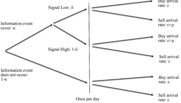
The Probability of Informed Trading (PIN) is computed on a simple model of information among traders [16]. Let’s describe it with the following tree below (Figure 1), originally designed in [16]. Suppose prior to the beginning of any trading day, Nature determines whether an information event is relevant to the value of the asset to occur. Suppose information events are independently dis-tributed and occur with a Bernoulli probability of value α , which can be seen on the first two branches on the left-hand side of the tree. These events are good news with a Bernoulli probability 1−δ (i.e. signal High), or bad news with probability δ _{(i.e. signal Low). After the end of trading on any day, and before} Nature moves again, the full information value of the asset is realized. Hence, for any of the three leaves of the tree in Figure 1, an informed trader would know which action to take. Trade arises from both informed traders (those who have seen any signal) and uninformed traders. On any day, arrivals of uninformed buyers and uninformed sellers are described by independent Poisson processes of respective intensity  and µ. Individuals trade a single risky asset and

money with a market maker over i=1,,I trading days. Within any trading

day, time is continuous and it is indexed by t∈

[ ]

0,T . Let’s define for t∈

[ ]

0,T ,

for a given trading day, St and Bt the events that an order of respectively a sell and a buy arrive at time t. Let Pt=

(

P nt

( ) ( ) ( )

,P bt ,P gt

)

be the market

maker’s prior belief about the events “no news” (n) “bad news” (b) and “good news” (g) at time t1_{. Within this model we compute the spread at t}

t

(4)

[image:4.595.219.533.75.253.2]

DOI: 10.4236/jmf.2019.94032 640 Journal of Mathematical Finance Figure 1. A tree summarizing the theoretical framework.

is willing to pay). Within this framework bt is the expectation of the asset value, we denote Vt, conditional on the history prior to t and on sell order St. Simi-larly, at is the expectation of Vt conditional on the history prior to t and on buy order Bt. Let note V ,

*

V and V respectively the value of the asset

under the conditions of good new, no information and bad new. We have of course the following inequalities: *

V ≤V ≤V .

2.2. Computation of the Spread

We explicit now more the content of [3]. Let’s compute the bid, the ask follows exactly the same idea2_:

(

| ,

)

.

t t t

b =E V t S

It can be re-written this way using the different possibilities of the tree on an event:

(

) (

)

(

) (

)

(

) (

)

(

)

(

)

(

)

*

| , , | | , , | | , , |

| | | .

t t t t t t t t t t t t t

t t t t t t

b E V t S n P n S E V t S g P g S E V t S b P b S

V P n S VP g S VP b S

= + +

Let’s compute the first term P n S_t

(

| _t

)

, others follow the same idea. Using Bayes rule one finds the following:

(

|

)

t

(

t|

_{( )}

)

t

( )

,

t t

P S n P n

P n S

P S

=

so, by decomposing the denominator:

(

|

)

₍

₎

_{( )}

₍

(

|

)

₎

( )

_{( )}

₍

₎

_{( )}

.

| | |

t t t

t t

t t t t t t t t t

P S n P n

P n S

P S n P n P S g P g P S b P b

=

+ +

Let’s have a look at the term P St

(

t|n

)

which is the probability at t that there will be a sell order at t under the constraints of no news. P St

(

t|n

)

is a transi-tion rate. To compute it, one must first calculate the transitransi-tion probability for a 2_{We use the same notations as the author, distinguishing the events “t” and “}

(5)

DOI: 10.4236/jmf.2019.94032 641 Journal of Mathematical Finance strictly positive time length let say h. Formally, if one notes Nt the number of jumps of the corresponding Poisson process up to t under conditions of no events, we know its intensity is t under the constraint of no news. For any h

strictly positive and small enough we look to the limit of the number

(

t t h 1 |

)

P N N n

h

−

− ≥

when h goes to zero remaining strictly positive, which de-fines the transition rate. At first order on h, one finds:

(

1 |

)

1 eh

( )

.

t t h

P N −N₋ ≥ n = −  =h o h+

Dividing by h, one re-finds indeed the intensity of the Poisson process, which is a special case of a Markov jump process. Applying the same for other cases (“bad event”, “good event”), we have finally the following:

(

)

( )

(

)

( )

(

)

( )

( )(

)

| | |

.

t t t t t t t t t

t t t

P S n P n P S g P g P S b P b

P n P g P b µ

+ +

= + + +

As the probabilities with  sum to one we get the following expression:

(

|

) ( )

(

|

) ( )

(

|

) ( )

( )

.

t t t t t t t t t t

P S n P n +P S g P g +P S b P b = + P b µ

Finally the bid has this expression:

( )

( )(

)

( )

*

.

t t t

t

P n V P b V P g V

b

P b

µ µ

+ + +

=

+

  



With the same reasoning the ask has this expression:

( )

( )(

)

( )

*

.

t t t

t

P n V P b V P g V

a

P g

µ µ

+ + +

=

+

  



Actually one may simplify a bit these expressions as the expectation of V has the following form:

( )

*

( )

.

t t t t

E V =V P n +VP b +VP g

We find:

( )

,

t

t t

VP b

b E V

P b P b

µ

µ µ

= +

+ +



 

and:

( )

.

t

t t

VP g

a E V

P g P g

µ

µ µ

= +

+ +



 

So the spread equals to:

( )

_{( )}

t

_{( )}

( )

t

_{( )}

( )

.

t t t t

VP g VP b

a b E V

P g P b P g P b

µ µ

µ µ µ µ

 

Σ = − = _ − _+ −

+ + + +

 

 

   

In the special case where P gt

( )

=P bt

( )

one finds the following simple form:

( )

(

)

( )

(

)

( )

(

1

)

(

)

.

2 1

t t

t

t t

P n P g

V V V V

P g P n

µ µ

−

Σ = − = −

+ + −

 

(6)

DOI: 10.4236/jmf.2019.94032 642 Journal of Mathematical Finance have the following:

(

)

thePIN

(

)

.

2

t V V V V

µα αµ

Σ = − = −

+



Thus, with the assumptions: P g_t

( )

=P b_t

( )

= = −δ 1 δ , i.e. 1

2

δ= and

( )

0

( )

1

t

P n =P n = −α, the PIN equals the following:

PIN .

2

µα µα =

+



We will keep the same hypothesis for the rest of the paper.

3. Analysis of the First Order Approximate within the

Time-Clock Framework

The idea behind the VPIN is to find an easy way to compute the last above ex-pression of the PIN using a volume-clock paradigm. More precisely, it aims at finding a way to easily compute the expressions obtained for the numerator αµ and denominator (αµ+2). The key heuristic behind the VPIN is to take

ad-vantage of a supposedly good property of the expectation of the absolute differ-ence between Poisson random variable within a volume-clock framework to approximate αµ, i.e.: E X

(

−Y

)

, where X and Y are Poisson variables. We

will see this heuristic does not really make it possible to conclude as expected. More precisely, in the first subsection we will see which idea has been used to approximate the PIN within a time-clock framework. Secondly, we will see that first-order approximations used are not correct as the framework does not ve-rify a required hypothesis. We analyze more precisely the first order approx-imates which can be made in the time-clock framework. In the third subsec-tion, we describe the volume-clock framework and explain why its hypotheses lead to different results compared to the time-clock framework. Finally, we illu-strate our results with simulations.

3.1. The Design of a New Heuristic

In the first subsection we see which idea has been used to approximate the PIN within a time-clock framework. We refer now to the related work of Easley et al.

[1]. Considering the previous framework the probability to obtain on the same time yt =

(

S B,

)

, S sells and B buys for day t of length one is:

(

)

(

)

(

)

( )

(

)

₍

₎

( )

(

)

2 2

2

, 1 e 1 e

! ! ! !

e .

! !

B S B S

t

S B

P y S B

B S B S

B S

µ

δ α α

µ αδ

+

− + −

− +

+

= = − + −

+ +

 



  

 

So, if one notes TT = +S B the total number of trades for this day, one finds,

conditioning by all possibilities of the model:

( )

(

1

) (

|

)

(

|

) (

1

) (

|

)

.

E TT =α −δ E TT g +αδE TT b + −α E TT n

(7)

DOI: 10.4236/jmf.2019.94032 643 Journal of Mathematical Finance

( )

(

1

)(

)

(

) (

1

)(

)

,

E TT =α −δ + + +µ  αδ µ+ + + −  α  +

i.e.

( )

2 .

E TT =αµ+ 

Note the following:

• _{Remark 1: the time period is fixed, thus S and B can take whatever possible}

positive integer values, which won’t be the case if S + B was fixed.

• _{Remark 2: intensities are rates, thus the equation has a meaning because one}

implicitly multiplies it by one (trading day).

The authors propose to compute the expectation of the absolute value of the following random number K = S − B with an approximate. This is the intuition behind the computation of the VPIN. They refer to the following paper of Katti

[17] but do not explicit any calculus. They assert that E K

( )

=αµ thanks to a

first order approximation without explaining what it does mean. Let’s first scribe the content of this reference and assumptions assumed. Then let’s de-scribe which computations are involved within this time-clock framework.

3.1.1. Katti’s Reference Assumptions

The reference proposes several ways to compute the expectation of the absolute value of two random variables that follow same discrete positive distribution but with possibly different parameters. The case of Poisson processes is treated. Let’s describe the beginning of Katti’s paper [17]. Let’s note X1 and X2 two Pois-son random variables of intensity λ1 and λ2. We would like to compute the following number ∆ =1 E X1−X2 . One can write the following:

(

) (

)

(

) (

)

1 2 1 1 1

,

1 2 2 2

,

1 2 2 1

, ,

|

,

i k

i i k i i k

i k i k

kP X X k X i P X i

kP P₊ kP P₊

∆ = − = = =

+ − = = =

= +

∑

where the summations are over 1, 2, 3, and 1 _e 1 1

!

i

P

i

λ λ −

= and 2 _e 2 2

!

i

P

i

λ λ −

= .

Then, one can develop it as follows:

(

)

(

)

(

)

(

)

1 2 1 2 2 1 2 1 1 2

1 1 2

0 0 0 0

e e ,

! ! ! !

i k i k

i i i i

k k

A B

i i k i i k

λ λ ∞ ∞ λ λ λ ∞ ∞ λ λ λ λ λ

− − − −

= = = =

 

 

∆ = _ + _= +

+ +



∑∑



with A1 and B1 the two different sums. The author, in order to simplify the calculus and use a trick, makes the following assumptions: λ λ1 2 =ν , where ν is a constant not linked anymore to λ2 nor λ1. It implies thus a relation be-tween the two variables (for example 1

2 1

λ λ

= _{). Thanks to this assumption he}

can do the following:

2

1 2 2 0

0 0

2 2

, !( )!

i k

A A

i i k

ν λ

δ δ

λ λ

δλ δλ

∞ ∞ = =

 

   

=_ __ _=_ _

+

 

∑∑

  

(8)

( )

(

)

0 2 1 2

0

1; 1; , !

i

A F i

i

ν _λ

∞ =

=

∑

+

where F1

(

α γ, ,x

)

is a confluent hypergeometric function. Operating by ( 2

2

δ λ

δλ ) it finally leads to:

2

1 2 0 1 1

2 2

3 1

e ;3; 4 ;1; 4 .

2 2

A λ ν A ν νF ν ν F ν

λ λ

  _ _ _ _

=_ − _ + _ − _+ _ − _

   

 

The particular case of λ1=λ2=λ cannot be treated with this trick because it would imply equal numbers are linked by an inverse relation, so that the product is independant of λ2. But λ λ1 = 2 = ν ,

ν

is not anymore a constant of the main parameters λ1 and λ2, so applying the operator does not give the pre-vious results. One may use here another reference, one cited by Katti [18]. We will detail later the same ideas for our precise the VPIN framework. Anyway, this case leads to the following:

( )

(

)

2

1 2 e I0 2 I1 2 ,

λ

λ − λ λ

∆ = +

where

( )

₍

₎

2

0 2

! !

n i

x

I x

i n i

+

∞ =

      =

+

∑

is a modified Bessel function of first kind.

3.1.2. How to Use as Far as Possible References’ Work to Approximate

the VPIN in a Time-Clock Framework

First, let’s put ourselves in the context where we have the differences of only Poisson processes. It’s pretty simple, one just have to condition the expectation of E K

( )

for each case:

( )

(

1

)

(

|

)

(

|

)

(

1

)

(

|

)

.

E K =α −δ E K g +αδE K b + −α E K n

Then, remind K= −S B. S and B are, under the model assumption, Poisson

processes describing the number of sells and buys in one day of trade. We only need two different kinds of Poisson processes to describe the mixture of Poisson processes resulting of informed and uninformed traders in each case (“good event”, “bad event” and “no event”). Let’s note them as follows X_S ~ 

( )

,

( )

~

B

X_   , B ~

( )

Y_µ  µ and S ~

( )

Y_µ  µ , S and B labelling buys or sells. One

finds then:

( )

(

)

(

)

(

)

(

)

(

)

1

1 .

S B B B B S

S B

E K E X Y X E Y X X

E X X

µ µ

α δ αδ

α

= − − + + + −

+ − −

   

 

As all Poisson processes are independant one can sum them to produce new Poisson processes, as follows3_:

( )

(

)

(

)

(

)

(

)

(

( )1 ( )2

)

1 1 .

E K =α −δ E X_−Y_µ₊_ +αδE Y_µ₊_−X_ + −α E X_ −X_

One can thus sum the two first terms and obtain the following:

(9)

( )

(

)

(

)

(

( )1 ( )2

)

1 .

E K =αE X−Yµ+ + −α E X −X

One has to treat finally two different cases:

• _{different intensities: first term} • _{same intensities: second term}

3.2. How to Reach a First Order Approximate

In this subsection we will first see that main assumption to use Katti’s result cannot be used to approximate the PIN. Therefore to approximate the PIN using authors’ intuition we describe then the following two steps:

• _{one way to reach numerator exact value consists in using Ramasubban’s ideas} [18],

• _{first order asymptotic analysis involves separate cases to study sensitivity of}

the approximate to parameter’s values.

3.2.1. Katti’s Assumptions Are Not Met in the New Setting

We have seen that Katti’s reference use the assumption that Poisson intensities are linked by a relation of the form 1

2

ν λ

λ

= _whereν_{is independent of these}

parameters. Here the respective parameters would be µ+ and . The

prod-uct  

(

+µ

)

has clearly no single reason to be a constant. One could create some tricky cases, but it does not seem that the model would like to be limited to these cases (indeed, one may consider for example to fit the PIN parameters maximising likelihood, like in [1]). Thus the assumptions are not met and the reference [17] cannot be invoked to say E K ≈αµ at first order, as it was done

in [1] for example.

3.2.2. Computation of E K

( )

Anyway, let’s do nevertheless calculations to compute E S

(

−B

)

. We follow

the same natural ideas of T. A. Ramasubban in this paper which treats only the case of same Poisson intensities [18]. We begin with:

(

)

(

)

(

1 2

)

1 αE X Yµ+ 1 α E X X .

∆ = _− _ + − _− _

Let’s start with the easier calculation: the case where Poisson intensities are equal.

(

)

(

) (

)

(

) (

)

(

)

(

)

(

)

(

)

1 2 1 2

,

1 2

0

2

0

1 1

2

* 0 1

2

2e

! !

2 e .

1 ! ! ! 1 !

i j

i

i j

i j i

i j

i j i j

i i

j j

i

E X X P X i P X j i j

P X i P X j i j

i j i j

i j i j

∈

∈ = −

∈ =

− −

−

= =

∈

− = = = −

= = = −

= −

− −

∑

∑∑

∑ ∑

∑



   

 



 

   



(10)

(

)

1 1

1 2 2

*

0 0

1 2

2 1 2

2

2 2 e

! ! ! !

2 e

! ( 1)! !

2 e .

!( 1)! !

i j i j

i i

i j _i j

i i i

i

i i

E X X

i j i j

i i i

i i i

+ − − ∈ = _∈ = + − ∈ + − ∈ ∈   − = _ − _      = _  ₊ + _       = _ + _ +  

∑∑

∑ ∑

∑

 _                    

One recognizes here a modified Bessel functions of first kind: for an integer n

and, say scalar x,

( )

₍

₎

2 2 ! ! i n n i x I x

i n i

+ ∈       = +

∑

 . Here we obtain:

(

)

2

(

( )

)

0 1

2 e 2 2 .

B S

E Y −Y =  − I  +I 

which is the result of Ramasubban’s quoted paper. The computation with dif-ferent intensities follow the same idea, expect that the symmetry of the two ini-tial sums is broken, so we have to compute them separately.

(

)

(

)

(

)

(

)

(

)

(

)

0 0 . i i j i i j

E X Y P X i P Y j i j

P X j P Y i i j

µ µ µ + + ∈ = + ∈ = − = = = − + = = −

∑∑

       

Let’s calculate the first sum and then the second:

(

)

(

)

(

)

(

)

(

)

(

)

(

)

(

)

0

2

1 0 1 1

1 1

2

0 0 1 0

e

1 ! ! ! 1 !

e , ! ! ! ! i i j j j i i i i

i j i j

j j

i i

i j i j

P X i P Y j i j

i j i j

µ µ µ µ µ µ µ + ∈ = +∞ +∞ − − = = = = + + +∞ + +∞ − − − = = = = = = −  ₊ ₊    = −  − −     ₊ ₊    = _ − _  

∑∑

            

which separates as follows as all sums exist separately:

(

)

(

)

(

)

(

)

(

)

(

)

(

)

0 1 ₁ 2 2

0 0 0

e e .

! ( 1)! ! 1 ! !

i

i j

i i j

i i i

i i j

P X i P Y j i j

i i i i j

µ

µ µ µ µ_µ µ

+ ∈ = + ₊ +∞ +∞ − − − − = = = = = −  ₊ ₊  ₊   = + −  +  +  

∑∑

∑

∑∑

    _      

Replacing first sum of the rigth hand side by Bessel functions of second kind, we finally find:

(

)

(

)

(

)

(

)

(

)

( )

(

₍

₎

)

(

)

(

)

0 2 1 0 1 2 0 0

e 2 e 2

e .

1 ! !

i i j j i i i j

P X j P Y i i j

I I i j µ µ µ µ

µ µ µ

µ µ + ∈ = + − − + +∞ − − = = = = − = + + + + + − +

∑∑

               

(11)

(

)

(

)

(

)

(

)

(

)

(

)

(

)

0 1 1 2 2

0 0 0

e e ,

! 1 ! ! 1 ! !

i

i j

i _i _i _i j

i

i i j

P X j P Y i i j

i i i i j

µ

µ µ µ_µ µ

+ ∈ = + + +∞ +∞ − − − − = = = = = −   + + = _ ₊ + _− ₊  

∑∑

∑

∑∑

    _       thus:

(

)

(

)

(

)

(

)

(

)

(

)

(

)

0 2 2 2 1 0 1 2 0 0

e 2 e 2

e . ! ! i i j i _j i i j

P X j P Y i i j

I I i j µ µ µ µ µ µ µ µ µ + ∈ = − − − − +∞ + − − = = = = − = + + + + + +

∑∑

∑

               

If we put together all the terms we find:

(

)

(

)

(

)

(

)

(

)

(

)

2 2 1 0 1 1

0 0 0 0

2

e 2 2 2

.

1 ! ! ! !

j i

i j

i i

i j i j

E X Y I I

i j i j

µ

µ µ µ µ

µ µ µ µ µ − − + + +∞ +∞ + = = = =  ₊  − = + + +  ₊   + +  − +  + _

∑∑

∑

               

Arranging the last two sums of the left hand side of the equality we finnaly get:

(

)

(

)

(

)

(

)

(

)

(

)

2 2 1 0 0 2

e 2 2 2

1 1 .

i

E X Y I I

P Y i P X i P X i

µ µ

µ

µ _µ _µ

µ µ − − + +∞ + =  ₊  − = + + +  ₊  +

∑

= ≤ + − ≥ +         _{ } _ _{ }  

Thus E K equals:

(

)

( )

(

)

(

)

(

)

(

)

(

)

(

)

2 0 1 2 2 1 0 0

2 1 e 2 2

2

e 2 2 2

1 1 .

i

E K I I

I I

P Y i P X i P X i

µ

α

µ

α µ µ

µ αµ − − − +∞ + = = − _ + _  ₊    + + + +  +    +

∑

= ≤ + − ≥ +           _{ } _ _{ }  

With an arbitrarily time length t for a trading period, we find:

(

)

( )

(

)

(

)

(

)

( )

(

)

(

)

(

)

2 0 1 2 2 2 1 0 0

2 1 e 2 2

2

e 2 2 2

1 1 .

t

t t

t i

E K t I t I t

t t

I t tI t

t

t P Y i P X i P X i

µ

α

µ

α µ µ

µ αµ − − − +∞ + = = − _ + _  ₊    + + + +  +    +

∑

= ≤ + − ≥ +                 

3.2.3. Analysis of the First Order Approximate

(12)

de-DOI: 10.4236/jmf.2019.94032 648 Journal of Mathematical Finance rived an asymptotic expansion of modified Bessel function of first kind as fol-lows:

( )

(

)(

)

( )

(

)(

)

( )

2 2 2 2

2 2 2

3

4 1 4 9

e 4 1

~ 1

8

2 2! 8

4 1 4 9 4 25

3! 8 z I z z z z z α α α α

α α α

 ₋ − −  − +  π   − − −  − +   

for z 1 and arg 2

z <π

We first apply this expansion to E K with the condition µ1 and 1,

as we consider there are a lot of informed and uninformed traders per day (compared to 1). We find the following:

(

)

(

)

(

)

(

)

( )

(

)

(

)

(

)

2 2 2 3 4 0

~ 2 (1 ) e

2

1 1 .

i

E K

P Y i P X i P X i

µ µ µ µ α α µ αµ + − − +∞ + = + + − +

π π ₊

+

∑

= ≤ + − ≥ +            

Let’s now distinguish these three cases:

• µ_and  are of same order,

• µ=o

( )

 ,

• =o

( )

µ ,

If µ_and  are of same order,

in this case:  

(

+µ

)

<2−µ, thus one can neglect the corresponding term.

We obtain:

(

)

(

)

(

)

(

)

0

~ 2 1 1 1 .

i

E K α αµ P Y µ i P X i P X i

+∞ + =

− + = ≤ + − ≥ +

π

∑

  



Thus PIN ~ 2

αµ

αµ+  and

(

)

(

)

0

(

)

(

)

(

)

2 1 1 1

~ .

2

i P Y i P X i P X i

E S B

µ α αµ αµ +∞ + = − + = ≤ + − ≥ + − _π + +

∑

     if _µ then it reduces to:

(

)

(

)

(

)

0

~ 1 1 .

i

E K αµ P Y _µ i P X i P X i

+∞ + = = ≤ + − ≥ +

∑

   Thus:

(

)

0

(

)

(

)

(

)

~ 1 1 .

2 i

E S B

P Y i P X i P X i

E S B µ

αµ αµ +∞ + = − = ≤ + − ≥ + + + _

∑

  

If µ=o

( )

 ,

we find:

(

)

(

)

(

)

(

)

0

2 1 1

~ .

2

i P Y i P X i P X i

E S B

(13)

And: PIN ~ 1

2

αµ



 .

If µ, then:

(

)

~ 1 .

E S B

−

+ _π

If =o

( )

µ ,

we find:

(

)

0

(

)

(

)

(

)

~ 1 1 .

i

E S B

P Y i P X i P X i

E S B µ

+∞ + =

−

= ≤ + − ≥ +

+

∑

  

and PIN ~ 1

Thus, we can see that first order approximation depends a lot of:

• _{the respective values of} µ and ,

• _{and in a lot of cases of the weighted average of a given Poisson distribution of}

the difference between cumulative density functions from opposite parts of the tail of another Poisson distribution, i.e.:

(

)

(

)

(

)

0 1 1

i P Y µ i P X i P X i

+∞ +

= = ≤ + − ≥ +

∑

  

The first order approximation E S−B ~αµ proposed in [1] is not incorrect as we will see in the simulations, but sometimes, imprecise.

3.3. The Volume-Clock Paradigm: The Implicit Change of Model Assumptions

In this subsection, we describe the volume-clock framework and explain why its hypotheses lead to different results the PIN compared to the time-clock frame-work. More precisely, we first describe the new assumptions. Secondly, we make the computations within this new framework, which lead to a new value of the PIN.

3.3.1. The New Assumptions

In [3] D. Easley, M. de Prado and M. O’Hara describe a new model to compute easily the VPIN and therefore the PIN using the above previous results:

• E S

(

−B

)

=αµ, supposedly at first order,

• E S

(

+B

)

=αµ+2

They introduce the paradigm of volume clock and time bars. Let’s first de-scribe it and see that the assumptions are implicitly changed, but ignored. The idea is pretty simple. Consider a trade described by a time serie of price, say pt, labelled with time t. First, They package trades in objects called “bars” that have a fixed time volume, i.e.: they aggregate the time serie in, for example, one-minute time bars. It is equivalent to a sampling of the time serie. Each bar is a kind of new trade with several rules to guess its price. Second they agreggate these time bars to form fixed in volum “buckets”. Say these buckets have a volume V.

• _{Remark 1: nothing can ensure us that buckets will have a fixed volume size.}

(14)

DOI: 10.4236/jmf.2019.94032 650 Journal of Mathematical Finance one wants to force bucket size to be constant then, a lot of time bar won’t be of one minute lenght. If one on the contrary wants to preserve time size to be constant, a lot of buckets might not be of constant volume size.

Suppose anyway that everything is ideal and that each bucket is of constant volume. Authors note τ the label of a bucket of volume V, V_τ, and V_τS and

B

V_τ respectively the total number of sells and buys that occured in this bucket.

They then refer to their previous work [1] result:

(

S B

)

E V_τ −V_τ ≈αµ. But even if

the result does not hold as previously shown, one must note the following:

• _{First: here the bucket is constant in volume, thus filling volume time is}

ran-dom, it is a really strong hypothesis, as we have then: S B

V_τ +V_τ =V that

holds almost surely,

• _{Second: they use the result indeed to say that as} S B

Vτ +Vτ =V then the

ex-pectation equals V =2+αµ.

• _{But finally, one should remark that this equality lacks a time, as we are}

talk-ing of rates of traders. In the first model, the time was one day, and implicitly one would multiply within the time-clock framework, rates by one day. Here, in the volume-clock framework, one does not control anymore time. One should take into account filling bucket time which is a new random variable. At first glance, the expression is inhomogenous and even if right, it is far from being trivial.

Indeed the authors preciss us “recall that we divide the trading day into equal-sized volume buckets and treat each volume bucket as equivalent to a pe-riod for information arrival”. It’s misleading. Recall that in the initial model time is fixed (one day) and thus volum is random. Here one has the contrary, volume is fixed and time is thus random. Let’s detail a bit more the calculus with the new assumptions. To do so let’s precise a bit more the new implicit framework.

3.3.2. A New Computation of

(

S B

)

t t

E V −V |V

In fact we want to compute now 1

(

|

)

S B

E V_τ −V_τ V

∆ = _{, as bucket volume is}

fixed. Note t−t′ the filling time of the bucket τ and then note the following:

(

)

(

)

1 | ,

tot tot tot tot

t t t t

E S S_′ B B_′ V

∆ = − − −

with tot t

S , Sttot′ , tot t

B and Bttot′ the Poisson processes of the total sell up to t and t′ and the total buys up to t and t′. One has in distribution the following:

• tot tot tot_,

t t S t t

S −S′ =N −′

• tot tot tot_,

t t B t t

B −B′ =N −′ where ,

tot S t t

N −′ and , tot B t t

N −′ are Poisson processes describing total sells and buys in the bucket labelled with τ . The variables being independent, we can thus write the following:

(

)

1 , , | .

tot tot

S t t B t t

E N ₋_′ N ₋_′ V

∆ = −

One must note that there is still the constraint of the volume of a bucket:

, , .

tot tot

S t t B t t

(15)

DOI: 10.4236/jmf.2019.94032 651 Journal of Mathematical Finance Thus, imposing one value, imposes the other. Let’s calculate ∆1. First, one can condition the events: “good event” (g), “bad event” (b) and “no event” (n):

(

)

(

)

(

)

(

)

(

)

1 , , , ,

, ,

1 | , | ,

1 | , .

S t t B t t S t t B t t

tot tot S t t B t t

E N N g V E N N b V

E N N n V

α δ αδ

α

′ ′ ′ ′

− − − −

′ ′

− −

∆ = − − + −

+ − −

On each event, one knows the distribution of , tot S t t

N −′ and , tot B t t

N −′. One can then re-write it the following way4_:

(

)

(

₍ ₎ ₍ ₎₍ ₎

)

(

₍ ₎₍ ₎ ₍ ₎

)

(

)

(

₍ ₎ ₍ ₎

)

,1 ,1 ,2 ,2

1

,3 ,4

1 | |

1 | .

t t t t t t t t

tot tot

t t t t

E N N V E N N V

E N N V

µ µ

α δ αδ

α

′ ′ ′ ′

− + − + − −

′ ′

− −

∆ = − − + −

+ − −

   

 

The two first terms corresponding to “good” or “bad events” are equal in dis-tribution, that’s why we have:

( ) ( )( )

(

,1

)

(

)

(

₍,2₎ ₍,3₎

)

1 | 1 | .

t t t t t t t t

E N N _µ V E N N V

α −′ + −′ α −′ −′

∆ = _ − _ + − _ − _

Before going further, let’s implement the joint probability density function of for example, sells and buys and respective filling bucket time t-t’ in the case of a bad event. Let’s note it f S B t t V b

(

, , − ′| ,

)

. Now, we synthetise and refer to the great ideas of the proof of Kin and Le [14]. Remark first the following:

(

, , | ,

)

(

, | , ,

) (

| ,

)

,

f S B t t V b− ′ = f S B V t t b f t t V b− ′ − ′

and as f V t

(

| −t b′,

)

follows a Poisson law of intensity

(

t t− ′

)(

2+µ

)

, then

(

| ,

)

f t−t V b′ classically follows an Erlang law with the following parameters

(

t t V′; , 2 µ

)

Γ − + . Second, as S+ =B V almost surely, we have the following

equalities:

(

, | , ,

)

(

| , ,

)

(

| , ,

)

,

f S B t t V b− ′ = f S t t V b− ′ = f B t t V b− ′

and:

(

, | ,

)

(

| , ,

) (

| ,

)

.

f S V t t b− ′ = f B V t t b f V t t b− ′ − ′

We know f V t

(

| −t b′,

)

~

(

2+µ

)(

t−t′

)

and considering for example a

continuous bounded function g, one can guess easily f B V t

(

| , −t b′,

)

compu-ting E g S V t

(

, | −t b′,

)

using that

(

)

(

, | ,

)

(

, | ,

)

E g S V t−t b′ =E g S S+B t−t b′ . We find a binomial law

; , 2

S V

µ

 

 ₊ 

 

 

 i.e.:

(

| , ,

)

(

| , ,

)

; , ; , .

2 2

f S V t t b f B V t t b S V B V µ

µ µ

   + 

′ ′

− = − = _ _= _ _

+ +

   

 

 

 

So finally:

(16)

(

, , | ,

)

; ,

(

, 2

)

.

2

f S B t t V b S V V µ

µ

 

′

− = _ _Γ +

+

 



 



The “no event” case is similar. We thus find the following:

(

)

(

) (

)

(

)

, , |

1

; , ; , 2 1 ; , ; , 2 ,

2 2

f S B t t V

S V t t V S V t t V

α α µ

µ

′ −

 

  _′ _′

= _ _Γ − + − _ _Γ − +

+

   



   

 And after an integration on the random variable t-t’:

(

)

1

(

)

, | ; 1 ; , .

2 2

f S B V α S V α S V

µ

 

= _ _+ − _ _

+

   



 



Taking the previous joint probability into account we are thus computing the following expectations of let say X and Y in fact:

(

)

(

)

(

)

1 αE V 2X 1 α E V 2Y

∆ = − + − −

with ~ ; ,1 2

Y _S V _

 

 and ~ , ,

2

X V S

µ

 

 ₊ 

 

 



Moreover, if x follows the binomail distribution of which p.d.f is 

(

x m p; ,

)

, then using Jensen inequality for the concave function y→ y we have:

•

(

)

(

)

(

)

(

)

1

2 2 2

2 4 1

2 2 1 2 1

E m x p p

E m x m p p

m m

 

− _ _ −

= __ − _ _ ≤ − + ≈ −

  for

large enough m and p differing from 1

2

• E m

(

2x

)

E m

(

2x

)

2p 1

m m

− −

≥ = − .

Thus, for large enough V:

1 2 1 0,

2

Vα

µ

∆ ≈ − +

+

  i.e.

1 .

2

V αµ

µ ∆ ≈

+



Thus the VPIN metric approximates the following for large enough n as shown by Kin and Le [14]:

(

)

1 |

VPIN ,

2

n

S B

V V _{E V} _V _V

nV V

τ τ _τ _τ

τ αµ

µ

=

− ₋

= ≈ ≈

+

∑



which is indeed different of PIN

2

αµ αµ+ =

.

3.4. Some Simulation Verification

(17)

3.4.1. Framework and Experience Tested

For purpose of illustration, we compare the empirical form of E B

(

₍

S

₎

)

E S B

−

+ with

the PIN and the asymptotic limit5_{found within the time clock framework for}

different cases of  and µ_{. It is pretty easy to do, as controlling ex-ante all the} parameters of the model one then just has to generate the appropriate Poisson processes to obtain all the values. We illustrate the results with three examples:

• =o

( )

µ and µ of same order than : we took =100 and

{

10000, 20000, 30000

}

µ∈ _,

• µ=o

( )

 and  of same order than µ: we took µ=100 and

{

10000, 20000, 30000

}

∈

 ,

•  of same order than µ_{: we took}6 _₌₁₀₀₀₀_and

{

10000, 2000, 30000

}

µ∈ _.

Remarks:

• _{We compute 20 values for each choice of}__and µ in the three cases above,

• _{For each of the 20 values, the empirical expectations are computed with an}

average of 10,000 values,

• _{To compute the sum}

(

)

(

)

(

)

0 1 1

i P Y µ i P X i P X i

+∞ +

= = ≤ + − ≥ +

∑

   ,

consi-dering the values of  and +µ, we have bounded the sum to i=100000, when probability values starts to be then very little.

3.4.2. Results

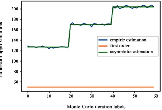
On each case, we plot first the empirical numerator E S

(

−B

)

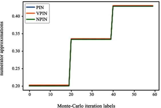
, αµ, and the

asymptotic limit found (Figure 2, Figure 4 and Figure 6). Second, we plot

(

)

(

)

E B S

E S B

−

+ , the PIN (i.e. 2

αµ

αµ+  and the asymptotic limit divided by

2

αµ+  (Figure 3, Figure 5 and Figure 7). Case1: =100,µ∈

{

10000, 20000, 30000

}

On Figure 2, first order and asymptotic estimations are very close. Case 2: µ=100,∈

{

10000, 20000, 30000

}

On Figure 3 and Figure 4, one can see better the difference when one does not change µ anymore.

Case 3: =10000,µ∈

{

10000, 2000, 30000

}

This last case on Figure 6 and Figure 7 illustrates a market where the number of informed and uninformed traders are of same order.

5 ( )

( )

(

)

( )

(

)

( )

(

)

(

( ) ( )

)

2

2 2

3 4

0

~ 2 1 e

2

1 1 .

i

E K

P Y i P X i P X i

µ µ

µ

µ α

α

µ αµ

+ − −

+∞ + =

+ + − +

π π ₊

+

∑

= ≤ + − ≥ +

  

   

  .

(18)

[image:18.595.234.518.69.258.2] [image:18.595.234.517.290.477.2]

DOI: 10.4236/jmf.2019.94032 654 Journal of Mathematical Finance Figure 2. Empirical, asymptotic and first order numerators.

Figure 3. Empirical, asymptotic and first order approximations of the PIN.

[image:18.595.237.517.510.700.2]

(19)

[image:19.595.235.518.68.258.2] [image:19.595.233.517.292.475.2]

DOI: 10.4236/jmf.2019.94032 655 Journal of Mathematical Finance Figure 5. Empirical, asymptotic and first order approximations of the PIN.

Figure 6. Empirical, asymptotic and first order numerators.

[image:19.595.233.517.508.700.2]

(20)

4. Another Suggestion to Compute the PIN

In this section, we propose another way to compute the PIN. Indeed, as it was seen in the last section, the first order approximation of the PIN within the time-clock is not always precise and its theoretical foundation is not correct. Furthermore, the one we propose is only asymptotic and not easy to compute. Hence we propose an exact formula to compute the PIN in the time-clock framework. More precisely, in the first subsection we describe how to compute exactly the numerator αµ_{and then the PIN. Secondly, we describe how} nu-merically one can design at least one methodology to compute the PIN. Finally, we present some simulation verification of our results.

4.1. One PIN Upgrade

In this subsection, we detail how to compute exactly the PIN. Recall that the probability to obtain S sells and B buys during a period of length t is:

(

)

(

)

(

)

( )

(

)

( )

₍

₎

( )

(

)

2 2

2

, 1 e 1 e

! ! ! !

e .

! !

B S B S

t t

t

S _B

t

t t t

P z S B

B S B S

t B S

µ

δ α α

µ αδ

+

− + −

− +

+

= = − + −

+ +

 



  

 

Recall that to compute the PIN we have the assumption: 1

2

δ = , thus we have:

(

)

(

)

( )

(

)

( )

(

)

( )

(

)

( )

2 2

2

, e e

2 ! ! 2 ! !

1 e .

! !

B S S B

t t

t

B S t

t t t t

P z S B

B S B S

t

B S

µ µ µ µ

α α

α

− + − +

+ −

+ +

= = +

+ −

 



   



So, if one notes TT= +S B the total number of trades for this day, we find:

( )

(

)

(

) (

1

)(

) (

2

)

,

2 2

E TT =α + +µ  t+α µ+ +  t+ −α  + t= αµ+  t

and we even have:

( )

.

2 2

E TT E S =E B =_ +αµ_t=

 

So to estimate the PIN denominator, one can first use for an arbitrary time pe-riod an average of S, B or TT. Let’s work with S and take a time pepe-riod of length t. Let’s estimate the numerator

2

t

αµ _{. To do this, we firstly explicit the margin}

probability function to obtain S sells in a time period of length t and secondly we compute its first three moments. Thirdly we explain how to compute α_and

hence the numerator, which finally leads to a new PIN formula.

4.1.1. Margin Function

(21)

(

)

( ) ( ) ( )

( )

(

)

( )

(

)

e 1 e e

2 ! ! 2 !

1 e e .

2 ! 2 !

S S S t t t t S S t t t t t

P z S

S S S

t t S S µ µ µ

α _α α

µ α α − + − − − + − + = = + − + +   = −_ _ +            

4.1.2. Computation of First Three Moments

Let’s compute the moment-generating function of this process. We will estimate the numerator using relations between moments. Let u be a real value, let VS be the random variable representing the volume of sells and t the fixed time pe-riod associated. We have:

( )

e 1 ( )

( )

e 1

e 1 e e .

2 2

u u

S t t

V u

E =_ −α_ − +α +µ −

 

 

Let’s compute the first three moments of VS:

• _{First moment:}

(

)

( )

e 1

(

)

( )

e 1

e 1 e e e e ,

2 2

u u

S t t

V u u u

S

E V =_ −α_ t − +α +µ t +µ −

      so:

( )

. 2 S

E V =_ +αµ_t

 

• _{Second moment:}

(

)

( )

(

)

( )

(

)

( )

e 1 2 e 1

2 2

e 1 2 ₂ e 1

e 1 e e 1 e e

2 2

e e e e ,

2 2

u u

S

u u

t t

V u u u

S

t t

u u

E V t t

t µ t µ

α α

α _µ α _µ

− − + − + −     = −_ _ + −_ _     + + + +         so:

( )

2

2 2 2_,

2 2

S

E V =_ +αµ_t+_αµ + +αµ _t

     

i.e. we have the classic decomposition:

( )

2

( )

(

)

1 .

S S S S

E V =E V +E V V −

• _{Third moment:}

(

)

( )

(

)

( )

(

)

( )

(

)

(

)

( )

(

)

(

)

( )

e 1 2 e 1

3 2

e 1 e 1

2 ₂ 3 ₃

e 1 2 ₂ e 1

e 1 e 1

2 ₂ 3 ₃

e 1 e e 1 e e

2 2

2 1 e e 1 e e

2 2

e e e e

2 2

2 e e e e ,

2 2 u u S u u u u u u t t

V u u u

S t t u u t t u u t t u u

E V t t

t t t t t t µ µ µ µ α α α α

α _µ α _µ

− − − − + − + − + − + −     = −_ _ + −_ _         + _ − _ + −_ _     + + + + + + + +                 so:

( )

2 3

3 2 2 3 3 2 3 2 3

3 ,

2 2 2 2 2

S

E V =_ +αµ_t+ _αµ + +αµ _t +_ + αµ + α µ +µ α_t