A single station method for the detection, classification and location of fin whale calls using ocean bottom seismic stations

A single-station method for the detection, classification

and location of fin whale calls using ocean-bottom

seismic stations

LuisMatias1,a)and DanielleHarris2 1_{Instituto Dom Luiz, Faculdade de Ci^}

encias, Universidade de Lisboa, Ed. C8, piso 3, 1749-016 Lisbon, Portugal

2

Centre for Research into Ecological and Environmental Modelling, The Observatory, Buchanan Gardens, University of St. Andrews, St. Andrews, Fife KY16 9LZ, United Kingdom

(Received 26 July 2014; revised 17 May 2015; accepted 7 June 2015; published online 24 July 2015)

Passive seismic monitoring in the oceans uses long-term deployments of Ocean Bottom Seismometers (OBSs). An OBS usually records the three components of ground motion and pres-sure, typically at 100 Hz. This makes the OBS an ideal tool to investigate fin and blue whales that vocalize at frequencies below 45 Hz. Previous applications of OBS data to locate whale calls have relied on single channel analyses that disregard the information that is conveyed by the horizontal seismic channels. Recently, Harris, Matias, Thomas, Harwood, and Geissler [J. Acoust. Soc. Am.

134, 3522–3535 (2013)] presented a method that used all four channels recorded by one OBS to derive the range and azimuth of fin whale calls. In this work, the detection, classification, and rang-ing of calls usrang-ing this four-channel method were further investigated, focusrang-ing on methods to increase the accuracy of range estimates to direct path arrivals. Corrections to account for the influ-ences of the sound speed in the water layer and the velocity structure in the top strata of the seabed were considered. The single station method discussed here is best implemented when OBSs have been deployed in deep water on top of seabed strata with lowP-wave velocity. These conditions maximize the ability to detect and estimate ranges to fin whale calls.

VC _{2015 Acoustical Society of America. [http://dx.doi.org/10.1121/1.4922706]}

[AMT] Pages: 504–520

I. INTRODUCTION

Monitoring marine mammals using static acoustic sen-sors is a common practice but a costly one, particularly in the deep ocean. For this reason, datasets acquired for other purposes, such as seismic monitoring, are extremely useful and valuable. Ocean bottom seismometers (OBSs) usually sample data at 50 to 100 Hz, so are suitable for recording low frequency calls of large baleen whales such as blue (Balaenoptera musculus sp.) and fin whales (Balaenoptera physalus) (McDonald et al., 1995). The large number of past, ongoing, and planned passive seismic experiments, along with the increasing number of available OBSs, provide a substantial dataset has been underutilized for marine mam-mal studies, until recently (e.g., Rebull et al., 2006; Wilcock, 2012).

It is possible to use OBSs for the location of sound sour-ces in the ocean, in addition to their primary function of identifying and localizing seismic events. A number of dif-ferent localization methods have been used to localize and track blue and fin whale with OBSs. Multipath differences can be used for ranging purposes from single OBSs and multi-station techniques can also be used for source location (e.g., Rebull et al., 2006; Wilcock, 2012; Weirathmueller and Wilcock, 2013). However, multi-station methods require that sensors are located close together (typically a maximum

spacing of 10 to 15 km) and multipath ranging with a single sensor does not allow the two-dimensional (2D) location of the sound source to be estimated. In addition, location of sound sources in the ocean is more complex than in tradi-tional crustal seismology due to the effects of oceanic sound velocity profiles on sound propagation.

Recently, it has been shown that an alternative single station method can be used for fin whale call localization at close ranges and with sufficient precision to be used in ani-mal density estimates (Harriset al., 2013). The basics of this method and its application to the localization of fin whale calls are presented inHarriset al.(2013). The main features of the method are (i) the method only works for direct path vocalizations from sources that are inside a critical range. The critical range is a function of the sound speed in the water column and theP-wave velocity in the top strata of the seabed; (ii) the seismic signal recorded by a three-component seismometer is used to estimate the apparent emergence angle of the P-wave in the seabed by applying the polarization analysis method of Roberts et al. (1989); (iii) the top seabed strata properties (includingS-wave prop-erties) are then used to convert this apparent angle to the true incident angle of the acoustic sound wave at the seafloor; (iv) this latter angle, and water depth, are finally used to esti-mate the location of the sound source considered to be close to the sea surface.

Here, the presentation of this single sensor method (SSM) is expanded, detailing the methodologies used for detection and classification of fin whale vocalizations and

a)

estimating ranges to calls. The effects that realistic sound propagation in both the water column and the top seabed strata have on the estimated ranges are also discussed.

InHarriset al.(2013)the feasibility of the SSM to esti-mate true ranges to sound sources close to the surface was validated by the analysis of airgun shots recorded in the Gulf of Cadiz during the NEAREST (2012) passive seismic experiment. Here, the same dataset is used to examine the performance of the detection, classification, and ranging methodologies in more detail. In addition, another dataset recorded in the Azores will be used to further validate the methodology using independently located fin whale vocal-izations using closely spaced sensors.

The paper is laid out as follows. Section IIrevisits the methodology, expanding the work presented byHarriset al.

(2013) to further explore the algorithms used to detect and classify fin whale vocalizations. Section III describes the control datasets, the analyses conducted, and gives the results. Finally, Sec.IVis an overarching discussion of the results obtained, ending with some general conclusions.

II. THE SINGLE STATION METHOD REVISITED

There are two main motivations for further investiga-tion of the detecinvestiga-tion, classificainvestiga-tion, and localizainvestiga-tion algo-rithm presented in Harris et al. (2013). First, the method will return spurious range estimates for direct path calls originating from outside the critical range or any multi-pathed signal. Therefore, it is important that the algorithm minimizes the probability of generating such ranges by selecting direct path calls that are strictly inside the critical range. Second, further consideration of the seabed and water properties is likely to lead to more accurate range estimation. The removal of false ranges and improving the accuracy of the remaining true ranges are both particularly important if the data are to be used for distance sampling, a standard animal density estimation approach (Buckland

et al., 2001;Harriset al., 2013).

A. Automatic detection of fin whale calls

Fin whales produce a variety of sounds (Thompson

et al., 1992) but the “20-Hz” call is the most studied fin whale vocalization and has been recorded worldwide (Sirovic´ et al., 2007; Stafford et al., 2009; Nieukirk et al., 2012). Each call is 1 s in duration, sweeping downwards over a 15–30 Hz range. Source levels above 180 dB re. 1lPa at 1 m have been estimated (e.g.,Watkinset al., 1987). The calls are repeated in series with a regular interval of several seconds (ibid.). These characteristics make fin whale calls particularly suited to analysis by conventional seismological methods and they can be easily detected by ocean bottom sensors, including OBSs. In fact, in the Gulf of Cadiz, fin whale calls constitute the strongest source of noise as recorded by hydrophones and vertical geophones in the fre-quency band from 2 to 30 Hz (Corela, 2014).

1. Cross correlation using a matched filter

The 20 Hz call is a repetitive down sweep with an am-plitude envelope displaying an asymmetric half-sinus shape (with energy slightly displaced to the front of the pulse). The amplitude and spectral band characteristics have been used byWilcock (2012)to automatically detect fin whale calls. In contrast, the method presented here uses a matched filter method that relies on the high repeatability of the vocaliza-tions and uses one of the loudest and highest signal to noise ratio (S/N) pulses selected from the data as the master wave-form. The cross-correlation of a running time-window and the master waveform is computed and only the windows that show a normalized correlation above a pre-defined threshold are saved for further analysis.

Very early in the development of the method it was noted that the application of the matched filter using the standard expression for the normalized correlation (CSxy) between two

arbitrary time seriesxiandyi[Eq.(1)] resulted in a very large number of detections with good correlations but very small absolute amplitude (equivalent to very small S/N),

CSxy ¼

X

xiyi

ffiffiffiffiffiffiffiffiffiffiffiffiffiffiffiffiffiffiffiffiffiffiffiffiffi X

x2i

X

y2i

q : (1)

Fin whale vocalizations have been shown to have a high source level with some variability (e.g., Sirovic´et al., 2007, estimated a mean source level of 189 dB re: 1lPa at 1 m over 15–28 Hz with a standard deviation of 4 dB).Weirathmueller

et al.(2013)showed that this source level is nearly constant between geographical locations. Since sound level attenuates with distance, it can be assumed that, in general, small ampli-tude signals will be likely generated by farther away sources or multipathed signals. However, such signals will generate spurious range estimates and so are unsuitable for analysis by the SSM. Therefore, the normalized correlation (CM

xy) formula

was modified as follows:

CM_xy ¼ pffiffiffi2

X

xiyi

ffiffiffiffiffiffiffiffiffiffiffiffiffiffiffiffiffiffiffiffiffiffiffiffiffiffiffiffiffiffiffiffiffiffiffiffiffiffiffiffiffiffiffiffiffi_X

x2i

2

þ Xy2i

2 r 0 B @ 1 C A M ; (2)

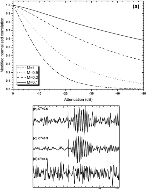
whereMis a constant to be chosen by the analyst.

Ifxi¼yi, this correlation also gives a value of one [as Eq.(1)], but when one of the pulses is attenuated by a factor, e.g.,yi¼Axi, then

CMxy ¼

ffiffiffi 2

p 1

ffiffiffiffiffiffiffiffiffiffiffiffiffiffiffiffi

A2_þ 1

A2 r 0 B @ 1 C A M : (3)

cross-correlation (hereafter referred as Cmax) may be set to a conservative value (typically 0.3 to 0.4). A number of diag-nostic parameters are then computed for each detected pulse in order to further identify direct path calls within the critical range, which are discussed in Sec.II B. Given that the modi-fied normalized correlation is affected by the relative ampli-tudes, it is important that the master signal used for the matched filter is chosen as having the largest amplitude expected in the time series to be investigated. In the two case studies investigated, the master signal was chosen as the call with the largest amplitude, confirmed by visual inspection.

2. Rejecting multipaths—using a time buffer

Since the SSM only works at close ranges (inside the critical range) where multipath pulses arrive a few seconds after the direct path, an additional parameter can be used to reject multipath arrivals. A “protection time buffer” DtPis defined, inside which only the largest correlation is kept. This method prevents a very large number of unwanted detections from entering the classification procedure. However, the use of this parameter may mean that a direct

path call produced shortly after another direct path call is rejected. Therefore, this parameter may be best used for the preliminary evaluation of the data when the classification pa-rameters are being fine-tuned. When the classification proce-dure is defined, then this time buffer can be relaxed so that multiple whales calling simultaneously in the same area can be investigated.

B. Classification of fin whale calls

Fin whale calls classified for use with the method must not only be (1) direct path signals, but must also be (2) within a critical range. In this section, the relationship between the horizontal and vertical velocities and the influ-ence of water column and seabed properties on the critical range are described in detail. A number of useful parameters that can be used to classify direct path fin whale calls are identified, as well as exploring whether multipath signals are likely to be misclassified as direct path signals.

1. The coherency factor

As explained in Harris et al. (2013) the polarization analysis of the seismic signal recorded by the three-component seismometer is performed using the method of Roberts et al. (1989), which uses the cross-correlation between the horizontal and vertical channels. The particle velocity that is recorded by the seismometer is defined as a vector,~vðtÞ,

~vðtÞ ¼ _ xðtÞ

_ yðtÞ

_ zðtÞ

2 4

3

5: (4)

In the absence of noise or phase shifts generated by local heterogeneities and scattering, the three velocity components should be perfectly correlated with constant coefficients a

andbthat depend exclusively on the azimuth/and apparent incident angleiapp,

_

xðtÞ ¼aPðtÞ _

yðtÞ ¼bPðtÞ _

zðtÞ ¼PðtÞ

a¼tanðiappÞsin/

b¼tanðiappÞcos/:

(5)

In order to assess the quality of the estimated parameters /

andiapp,Robertset al.(1989)proposed the computation of a coherency factor CO. If there was a perfect correlation between the horizontal and vertical velocities recorded by the seismometer, then

_ h tð Þ ¼

ffiffiffiffiffiffiffiffiffiffiffiffiffiffiffiffiffiffiffiffi

_

x2þy_2¼

q

_

x tð Þsin/þy t_ð Þcos/;

_

z tð Þ ¼ h t_ð Þ

tanðiappÞ

¼x t_ð Þ sin/

tanðiappÞ

þy t_ð Þ cos/

tanðiappÞ

: (6)

Equation(6) can then be used to estimate the vertical signal from the horizontal recordings

_

zestðtÞ ¼AxðtÞ þ_ ByðtÞ_ (7)

The predicted coherency factorCOis then defined by FIG. 1. (a) Attenuation that results from the application of the modified

CO¼1hðz t_ð Þ Ax t_ð Þ By t_ð ÞÞ

2

i

hz_;zi_ ; (8)

where hi means the series average. For a noiseless and ideally linearly polarizedP-wave signal this coherency fac-tor should be equal to one. In the other circumstances, the coherency factor is smaller than one. Therefore, using the Robertset al.(1989)method, a measurement of azimuth and apparent incident angle may be accepted whenever the coherency factor is larger than a predefined threshold.

2. The Zoeppritz equations and the critical range

To locate a sound source close to the surface from the seismic signals recorded at the sea-bottom, the true emergence angle has to be estimated from the apparent emergence angle of theP-wave in the top seabed strata. This relationship can be obtained by solving the Zoeppritz equa-tions that depend on the elastic properties of the water layer and seabed, considered as vertically layered isotropic media (e.g.,Aki and Richards, 1980).

The use of Zoeppritz equations are a common tool used in seismic exploration for amplitude versus offset analysis (e.g., Castagna, 1993). However, this formulation is strictly valid only for plane waves propagating with an infinite fre-quency. It has been recognized that departures from ampli-tudes derived by the Zoeppritz equations do occur when band limited signals from point sources are considered (e.g.,Favretto-Cristiniet al., 2007). We will begin by assum-ing that the conditions at the seafloor where OBS recordassum-ings are obtained meet the assumptions required by the Zoeppritz equations. Departures from these conditions will be addressed in Sec.IV.

Taking 20 Hz as the reference frequency for the fin whale calls and 2000 m/s as a typical value for the P-wave velocity in the shallow rocks, then the wavelength of the acoustic signal in the seabed is typically 100 m. The radius of the first Fresnel Zone (where reflected energy is reflected in phase) is then25 m. This implies that estimating the am-plitude of the recorded signals requires knowledge of the properties of the top seabed strata, down to25 m below the water-seabed interface.

The physical properties of the seabed are very difficult to measure directly from samples because, if the seabed is made of sediments, samples are very soft, highly saturated in water, and are not recoverable by usual coring techniques. Using laboratory andin situmeasurementsHamilton (1976) proposed a set of regression laws for the shear velocity in sediments composed of sand or silt-clay where, in the first 25 m of sediments, S-wave velocities (Vs) are predicted to range from 128 to 300 m/s. For compressional waves, Hamilton (1976)reports estimates for fine and coarse sands where theP-wave velocity (Vp) for the first 20 m range from 1700 to 1900 m/s. Taken together, these results point to a very high Vp/Vs velocity ratio, exceeding ten, for the shal-lowest sediments in the ocean floor. In comparison, in terres-trial sediments and hard rock the Vp/Vs velocity ratio rarely exceeds a value of 2.0 (e.g., Aki and Richards, 1980) and

water saturated sediments typically have a ratio of 3.0 at 1000 m depth below the seafloor (Hamilton, 1976).

Sediment density must also be considered. Measurements published by Nafe and Drake (1963) for marine sediments show values that range from 1.3 to 2.0 g/cm3 for P-wave velocities between 1500 and 2000 m/s.

When an acoustic plane wave impinges the ocean floor from above, the amplitudes of the reflected P-, transmitted

P-, and transmitted S-waves are characterized by three reflectivity coefficients. These can be obtained by solving the Zoeppritz equations for the elastic parameters that are typical for soft sediments found at the seafloor. When the reflectivity coefficients for this typical model are examined, it can be concluded that all of them (reflection and transmis-sion), have an imaginary part after some critical incident angle. The value of this critical angle depends on theP-wave velocity of the top seabed strata but not on theS-wave prop-erties and is obtained by

for a2 >a1; sinic¼ a1

a2

: (9)

Beyond this critical angle the emergence angle in the seabed also becomes a complex number that cannot be estimated from seismic observations. Thus, the single station method described here when applied to fin whale calls is limited to incidence angles smaller than ic. This also means that for a given source height,hw, above the sea floor and assuming a straight line propagation in the water layer, the method will be limited to horizontal ranges smaller than the critical range

Rcgiven by

Rc¼hwtanic: (10)

For example, in an environment wherea1, the P-wave velocity in the water column, is 1500 m/s and, a2, the

P-wave velocity at the seabed is 1800 m/s, then the critical angle is 56.4.

3. Identifying signals within the critical range

The theoretical amplitude of horizontal and vertical ground motion recorded by the seismometer can be easily computed from the reflectivity coefficients and from the hor-izontal and vertical slowness for each wave (Aki and Richards, 1980). According to plane wave theory, the verti-cal amplitude decreases sharply close to the critiverti-cal angle while the horizontal amplitude is null for a vertical incidence and increases constantly up to the critical angle.

The loss of correlation and coherency for post-critical incidence angles between the vertical and horizontal chan-nels in the seismometer is also observed between the vertical and hydrophone channel (Fig.2). This observation suggests three additional parameters that could be used to classify fin whale calls as being inside or outside the critical range: (i) CZH—the maximum normalized cross-correlation observed between the hydrophone and vertical channels; (ii) iZH—the time lag (in samples) for which the CZH above is observed; (iii) CZH0—the normalized cross-correlation observed between the hydrophone and vertical channels at zero time lag.

Another classification parameter that could be used is the S/N. For a constant noise background, this would be analogous to an amplitude threshold. In addition, its use would avoid the use of location estimates in the presence of large levels of noise in the seismometer. Ocean bottom seis-mic recordings, including the frequency band where fin whale calls are recorded, are mostly affected by oceanic swell, wind waves, bottom currents, and passing ships (e.g., Webb, 1998). The ocean bottom currents are mostly tide controlled and the noise conditions due to them are site de-pendent. The currents interact with the OBS parts inducing Von Karman vortices and resonance of the instrument with the seafloor (e.g.,Kasaharaet al., 1980;Corela, 2014) at fre-quencies above 2 Hz. The hydrophone records are unaffected by this current induced noise but the OBS channels could be affected, which could reduce the accuracy of other estimated selection parameters, highlighting the utility of including the S/N as an additional classification parameter.

In all implementations of this single station method, sig-nal amplitudes are measured by calculating the root-mean-square (rms) of the detected pulse. The noise level is also computed as the rms of the signal in a time window of the same length as the master waveform that precedes a given detected pulse. Noise and signal amplitudes for all four channels are stored during the detection process so that they can also be used for classification.

4. Identifying multipathed signals

Multipath arrivals must also be considered in the classifi-cation process. Despite the use of a protection time buffer, multipath arrivals may be accepted by the detection algo-rithm. To investigate the potential inclusion of multipath arrivals in the detection and classification processes, synthetic seismograms were computed. The seismograms simulated recordings by a seismometer at the sea floor below a water layer 4000 m thick using the seismic reflectivity method as modified byWang (1999). For the first seabed layer, typical values for the elastic parameters were used: a1, theP-wave

velocity in the water column, was 1500 m/s, a2, theP-wave

velocity in the shallowest seabed layer, was 1800 m/s,q1, the

water density, was 1.0 g/cm3, b2, the S-wave velocity in

the seabed, was 200 m/s, and q2, the seabed density, was

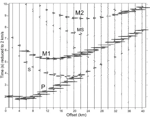
1.5 g/cm3. Some layering in the seabed down to 6 km depth was also included to replicate more realistic conditions at the seafloor. The synthetic seismograms for the vertical velocity, at 2 km spacing, are shown in Fig.3. The travel time has a lin-ear move-out correction with a velocity of 2 km/s to facilitate the visualization of all significant waves.

Under this model, direct path arrivals dominate the re-cording up to a range offset of 18 km (Fig.3). Beyond this distance the seismogram is dominated by the first multiple and the second multiple dominates beyond a range of 40 km. However, true amplitudes of multiples are considerably atte-nuated beyond 10 km, by over20 dB (this is not shown in Fig. 3due to the relative amplitude scaling applied). These results suggest that: (1) at ranges smaller than the critical range, multipaths will have a small amplitude and so they can be removed by the detection threshold or by another amplitude-based classification parameter, such as S/N and (2) at larger range offsets where first and second multiples

FIG. 2. Fin whale calls recorded by one seismometer showing well-correlated hydrophone (H) and vertical signals (Z) on the right panel. The left panel shows one whale call where a clear delay and difference in shape (phase) can be seen between the horizontal (XandY), the hydrophone, and the vertical channels.

dominate, the range is so large that the reflections at the sea-floor occur at angles larger than the critical angle and so the detections will be removed because of the change in shape and differences in delay between the four component channels.

The success of the proposed methodologies in the re-moval of super-critical incidence angles and multipath arrivals from the detected pulses can only be evaluated by the analysis of a control dataset where the true location of the acoustic sources is known. This will be examined in Sec.III.

C. Water column properties

Once the incidence angle of the acoustic wave on the sea floor is estimated, simple trigonometry can be used to compute the horizontal range of the sound source, assuming that the water layer is homogeneous (as in Harris et al., 2013). However, since the ocean is stratified, ray paths in the water from a near-surface source will curve considerably on their way down (concave down). When the seismic sensors are placed in deep water, this effect is expected to be large. However, the classification process should discard whale calls at range offsets larger than the critical range and for the small ranges considered by the method, the effect of ray bending by propagation in the water column is likely to be small. This was demonstrated using data from one of the test sites at the Gulf of Cadiz. In the validation analyses, the stratification of the water layer was taken into consideration.

III. TESTING THE SSM WITH SOURCES OF KNOWN LOCATION

A. Introduction to the control datasets

Two datasets were used to assess the method—one involved airgun signals of known location (used as a proxy for fin whale calls) and the other dataset used fin whale calls that had been localized using standard time difference of ar-rival methods.

1. The active seismic survey in the Gulf of Cadiz revisited

As part of the NEAREST project, 24 OBSs were deployed in the Gulf of Cadiz where they recorded up to 11 months of continuous four-channel data, from August 2007 to July 2008. A description of the deployment, data recorded, and instrumental characteristics were given in Harris et al.

(2013)and will not be repeated here.

In September 2007, the ship R/V Atalante passed over OBS18 (4605 m water depth) and OBS19 (4287 m water depth) while producing airgun shots (Somoza et al., 2007). InHarriset al.(2013)this dataset was used to test and vali-date the method in its simplest form. Here, this analysis is extended with a more rigorous classification process and a more accurate ranging process, applying knowledge of water stratification and a model for the elastic parameters in the top strata of the seabed.

However, it is important to note that an airgun source used for active seismic surveying is not a perfect model for fin whale calls. While the frequencies of fin whale calls are

well represented in the airgun shots, there are several key differences between the two signal types. Airgun shots have a much broader frequency spectrum and have higher energy content than the fin whale calls, affecting S/N and amplitude considerations. Furthermore, the shape of an airgun shot is different from a fin whale call. For example, while it is easy to identify on a seismogram the beginning of an airgun shot, it is not possible to do the same for fin whale calls. Finally, while the radiation pattern of a fin whale call is expected to be omnidirectional (Payne and Webb, 1971), the artificial sources used in seismic surveys are usually made of arrays of airguns tuned in such a way to focus the energy radiation vertically downwards. Therefore, it is expected that ampli-tudes from tuned airgun arrays will decay faster with range than fin whale calls. This is why it was important to also val-idate the method using a control dataset of fin whale calls.

2. The Lucky Strike dataset

The MOMAR (“Monitoring the Mid-Atlantic Ridge”) project was initiated by the international InterRidge Programme, to study active mid-ocean ridge processes along a slow-spreading ridge section. Multidisciplinary studies have been conducted to follow up the long-term evolution of hydrothermal environments at the Mid-Atlantic Ridge near the Azores (35N to 40N), in the Lucky Strike area. As part of the MoMAR monitoring effort, the Lucky Strike area has been continuously occupied by seismic sensors. The OBSs are periodically deployed and recovered at least once every year. The area has also been investigated by active seismic methods and the results regarding the local seismicity, geol-ogy, and crustal structure have been regularly published (e.g., Arnulf et al., 2011; Crawford et al., 2013). Besides active and passive seismic data the MOMAR sensors also recorded fin whale calls (Chauhanet al., 2009).

The data analyzed in this work belong to the BBMOMAR–2, Broad Band experiment for Monitoring of the Mid-Atlantic Ridge, 2008 cruise that recovered five OBSs in August 2008, which were deployed in July 2007 by the BBMOMAR cruise at2000 m water depth. The sensors were deployed close enough to allow for the location of fin whale vocalizations using conventional seismic triangulation methods (e.g., Ottem€oller et al., 2011). The dataset made available by IPGP, Institut de Physique du Globe de Paris (Crawford, 2013) comprises a set of station coordinates and waveforms with time stamps already corrected for the meas-ured time drift after a one-year deployment. All instruments recorded at 62.5 Hz sampling rate to ensure 1-year continu-ous operation. Frequencies up to 28 Hz could be analyzed, which was sufficient to investigate the 20 Hz fin whale call.

B. Methods

1. Signal detection

water could be clearly identified. The airgun data were proc-essed using the modified normalized cross-correlation formula shown above withM¼0.5 [Eq.(2)] using recordings from the vertical channel. The detection threshold (Cmax) was set to 0.3. The master waveform used for the detection process was one of the loudest airgun shots recorded (430 ms duration).

It was of interest to estimate the critical range for the Gulf of Cadiz recordings. However, the P-wave velocity in the shallowest sediments, a2, was not known. Therefore,

assuming an average sound speed of 1.502 km/s in the water column, varying P-wave velocities in the sediments were assumed, resulting in several candidate critical rang esti-mates: 6.49 km (a2¼1.8 km/s), 5.53 km (a2¼1.9 km/s), and

4.88 km (a2¼2.0 km/s). These predictions were compared to the detection results to see which seemed the most plausible.

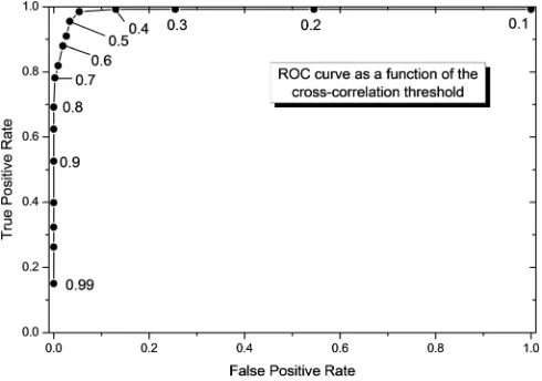
The receiver operating characteristic (ROC curve) of the detector as a function of the cross-correlation threshold was also calculated. The success interval was restricted to an ap-proximate critical range (5 km). True positive rate was cal-culated as the number of direct path signals originating within the critical range as a proportion of the total number of detections. In this analysis the false positive rate (FPR) was calculated as the number of false detections within the critical range as a proportion of the total number of false positives and true negatives. Any call originating from out-side the critical range was conout-sidered to be a false positive if detected, and a true negative if undetected.

Multipaths were considered to be true negatives/false positives in the classification process, regardless of the range at which they were produced. The true positive rate (TPR) as a function of range was also assessed for different values of Cmax [using the detection algorithm in Eq. (2) where

M¼0.5], initially without any classification applied. The TPR was calculated as the number of true positive detections performed over the total number of direct path shots inside a bin 1 km wide, allowing for 500 m overlap between bins for the Gulf of Cadiz dataset and 250 m overlap for the Lucky Strike dataset.

In the Lucky Strike dataset, recordings of fin whales at multiple stations were used to generate the control dataset against which the method was tested. Visual inspection of data showed that one of the strongest fin whale 20-Hz call sequences was recorded on November 30, 2007, between 08:00 and 10:00, for a 2-h period. The highest amplitude call from one OBS (LSo7) was chosen as the master waveform in the matched filter analysis. The choice was made due to the simplicity of the waveform and the absence of multipath arrivals. Call detection was performed using a matched filter as explained in Sec.II A, usingM¼0.5. A low detection cor-relation threshold (0.3) was used to ensure that most of the whale calls were detected. All detections on all five instru-ments were examined and corrected. OBS LSo7 provided the best quality signals and it was selected as the main call sequence to be processed using the single station method.

Next, all five individual call sequences were associated so that every single call could be identified in as many record-ings as possible (with a maximum of five occurrences). This process was done by visual inspection, profiting from the fact that fin whales travel slowly while vocalizing (e.g., 4–7 km/h

as reported in Rebull et al., 2006) and produce regular sequences of sounds interrupted by small gaps. The arrival times were manually re-picked at the onset of each pulse. Visual comparison of signals side-by-side facilitated the choice of a homogeneous picking point between different sta-tions. This procedure generated a total of 427 events, with most calls being recorded by four or five instruments.

By treating the calls as earthquakes located at or close to the surface, the 2D call locations were obtained using the SEISAN application (Ottem€oller et al., 2011), which per-forms seismological analyses. The velocity model in the water layer was derived from the conductivity, temperature, and depth (CTD) profiles recorded by the BBMOMAR cruise (Crawford et al., 2008). After a first location it was noted that some events diverted from the expected smooth path of a fin whale, and so events were examined to obtain an improved continuous path that represented the whale track. It was found that the conventional use of three decimal places to represent event locations inside SEISAN was not adequate for the analysis of these closely located sources, which occurred within a radius of 6 km. Therefore, the final location was obtained with a modified high-resolution code of the SEISAN location routine. Only identified pri-mary arrivals were used in the localization routine. The esti-mated locations were further improved by taking the running average coordinates of the neighboring four events for each location.

2. Signal classification

Both signal types (airgun shots and fin whale calls) were classified using the classification parameters presented above. Varying values for CO and iZH were tested. Preliminary tests showed that the CZH, CZH0, and S/N pa-rameters were not as useful asCOand iZH and so no results for these parameters will be presented. The TPR was assessed as a function of range for various classification pro-cedures. In order to assess whether the classification parame-ters were successful at reducing the number of false positives, which could include direct pulses from outside the critical range, the FPR was also estimated as a function of range. The FPR within each assessed distance was estimated by dividing the number of falsely classified signals (signals that were not direct paths inside the critical range) by the total number of false positives and true negatives across all ranges.

3. Water column properties

Outflow Water. This layer is likely to affect the sound propa-gation in the Gulf of Cadiz and it is shown to be present in the whole deep-water area where the NEAREST OBSs were deployed (e.g., Ambar et al., 2008). For this reason, this sound speed profile was considered a good approximation for the average conditions in the studied area.

Ray tracing was performed on the horizontally stratified water layer integrating the propagation equations by a simple Euler rule from the seafloor to the ocean surface.

C. Results

1. Signal detection

For this analysis, signals generated by the active shoot-ing up to an offset of 16 km were considered. A total of 427 airgun shots were fired within 16 km and a large number of multipaths were generated (n¼2090). In the OBS records, 346 shots were clearly identified as direct paths, 133 of which were generated inside a 5 km radius (representative of the critical range). The direct path arrivals of 81 shots, typi-cally produced at larger offsets, could not be identified in the OBS records at all. However, some of the detected multi-path arrivals may have originated from these shots.

A comparison of the amplitudes for the horizontal, verti-cal, and hydrophone channels as a function of the range off-set between the airgun shots and OBS19 is given in Fig.4. The comparison of the amplitudes in this way leads to sev-eral useful observations: (i) three domains as a function of range offset can be clearly identified: the small offset range, the critical distance range, and the far-offset range; (ii) the amplitude of the vertical (Z) channel decays as expected, almost reaching zero at the critical distance and after that, oscillating close to zero; (iii) the amplitude on the hydro-phone (H) channel also decays but never reaches a value close to zero; (iv) the decaying ofHamplitudes in the small offset range looks similar to what is expected for a free instrument with amplitude attenuating with geometrical dis-persion but this behavior changes drastically at critical distances and in the far-offset ranges; (v) all amplitudes

show strong oscillations at the critical range; (vi) the ampli-tude of the horizontal ground movement is zero at zero ranges and increases steadily thereafter. After reaching a maximum, it remains high up to the far-offset range where it decays continuously. The maximum amplitude is seen just after the critical distance as would be expected from the so-lution of the Zoeppritz equations; (vii) the amplitude varia-tions are not exactly centered at 0 km range offset reflecting

50 m uncertainty in sensor position after being relocated using the direct wave arrivals.

The high variability of amplitudes after the critical range supports the theory from Sec.IIand empirically dem-onstrates that the method is reliable only in the small-offset range. Examining the candidate critical distances displayed, it appears that the most plausible value for theP-velocity in the sediments is 1.8 km/s or very slightly slower.

The ROC curve showed that a 0% false positive rate was attained for a detection threshold of 0.8 or higher (Fig. 5). However, a considerable number (30%) of true shots were FIG. 4. Variation of airgun shot amplitudes with range offset (negative to the west). The horizontal channels are merged into a single horizontal measure. The hydrophone was scaled (divided by five) so that it could be compared with the vertical channel. Three sub-critical ranges are computed for three different

P-wave velocities in the sediments. Three range domains can be identified with different amplitude behaviors: the small offset range, the critical offset range, and the far offset range.

missed at that threshold level. Therefore, it may be preferable to use a conservative value for detection (e.g., 0.4) and design a classification scheme that preserves the true detections and filters out most (or all) of the false positives that originate both from inside and outside the critical range.

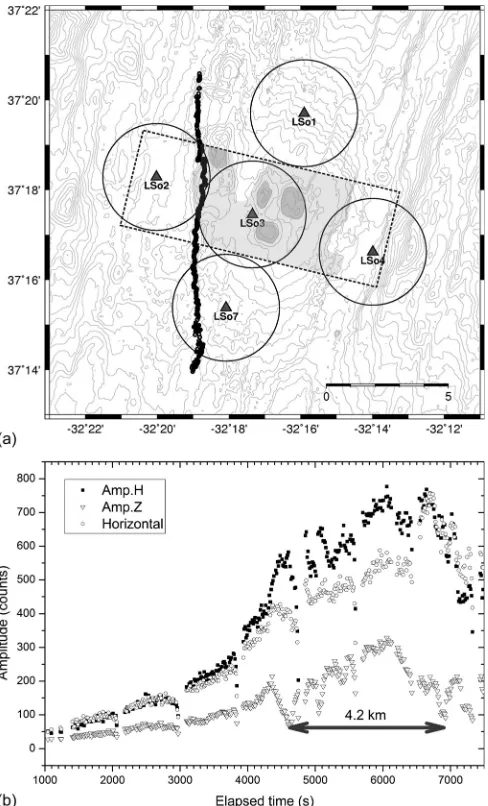
In the Lucky Strike dataset, OBS LSo7 generated 427 good quality calls and all the other sensors generated more than 390 whale calls. The number of fin whale call detection times available allowed the computation of 416 good 2D locations (out of 427 possible locations) with an average rms time error of 0.045 s. The resulting smoothed track ran roughly from north to south until the triangulation failed to

work due to the whale being too far from the center of the array [Fig.6(a)].

The amplitudes of the calls at far ranges (from 1000 up to 4300 s after the start of the time period of interest) increased continuously and smoothly as would be expected from the approaching of the fin whale to the sensor [Fig. 6(b)]. It was also clear in this time interval that the sound level generated by the fin whale dropped suddenly during the last calls of a sequence (i.e., at 2100, 3000, and 3800 s).

In theory, the amplitude of the vertical component (Z) should drop to zero at the critical range. This property ena-bles the critical range to be identified [Fig.7(b); from 4600 to 6900 s]. Since the whale track line did not directly approach LSo7 [Fig. 7(a)], the variation of amplitudes for the Z channel is not very large, but a slow increase then decrease can be seen, denoting the approaching and depart-ing of the sound source. The hydrophone amplitudes also show a slow variation, similar to the Z channel, except for elapsed times larger than 6400 s. An increase in amplitude is observed here, coincident also with an increase in the hori-zontal amplitude.

2. Signal classification

The performance of all classification parameters pre-sented in Sec.II Bwere investigated and the most promising were the polarization coherency (CO) and the correlation lag between Z and H channels (iZH). The variation of three-component coherency, CO, as a function of range, for direct wave arrivals inside a radius of 16 km is shown in Fig.7(a) for OBS19 and line MF12. A positive value ofCOgenerally identified the short-range domain except for near vertical incidence, or near-zero range, where, due to the small ampli-tude of the horizontal channels, the three-component coher-ency was poor. It was also clear that the maximum correlation (C.Max) from the detection process is very high for the near vertical incidence where CO was unreliable. Therefore, coherency can be a useful classification parameter if used conditionally; that is, calls should not be rejected usingCOif the correlation is high or if the estimated range is close to zero. This protection radius inside whichCO classifi-cation cannot be applied can be defined as a percentage of the sensor depth.

The variation of the lag for the maximum correlation between vertical and hydrophone channels with range offset, for direct wave arrivals, is shown in Fig.7(b)for OBS19 and line MF12. Due to the phase change at critical and super-critical incidence angles, the iZH parameter seemed to be a good discriminator to identify the short offset domain where reliable range estimates can be performed. However, some signals close to the critical range may be rejected and some far-offset calls may be retained.

For conservative values of the detection threshold (e.g., 0.3) shots produced beyond the critical range were easily detected. Undesired signals (i.e., shots outside the critical range) were only filtered out at a range close to the double of the critical range (Rc). For larger threshold values, the detec-tor filtered out signals at range offsets close to but smaller than Rc. This behavior is the one expected based on the FIG. 6. (a) Location of the five sensors deployed in the Lucky Strike area

variation of amplitudes of the Z channel with range offset (Fig.8). However, at range offsets larger thanRc, coinciding with an increase in theZchannel amplitude, the detector was unable to filter out a number of undesirable signals. Without using any other selection criteria, the TPR at7 km could be reduced by increasing the detection threshold, but with the effect of reducing the number of true classifications inside the critical range.

Several classification values were tested for the Gulf of Cadiz active seismic survey and it was found that iZH1 was a good discriminator. The detector performance at close ranges did not alter but signals originating beyond the critical range were more successfully rejected [Fig.8(b)]. However, a small and undesirable window for positive detections beyond the critical range remained at7 km range offset.

The polarization coherency between the vertical and hori-zontal channels, CO, was the other classification parameter that performed best to reject signals from outside the critical range, using aCO0.3 as a threshold and a protection radius (whereCOclassification was not used) of 250 m [Fig.8(c)].

Finally, the classification results were improved when both parameters were used together [Fig.8(d)]. It seems that

the two criteria reject different pulses and so the perform-ance of the classifier at range offsets larger thanRcwas con-siderably improved.

The FPR was only calculated for the classifier that joined the iZH andCOclassification parameters [Fig.8(e)]. The FPR was small (<0.003) for distances larger than 5 km and for a detection threshold of 0.4 or larger.

The results for the detection and classification of the fin whale calls at the Lucky Strike site were very similar to the results from the Gulf of Cadiz dataset [Figs.9(a)–9(c)].

For the lowest thresholds examined (Cmax¼0.5, 0.55) calls produced from beyond the critical range (RC¼2.0 km for a P-velocity in the sediments of 2.1 km/s) were easily detected. For larger values of the threshold, the detector started to filter out calls at range offsets close to, but smaller than, RC. At offsets larger than RC, coinciding with an increase in the Zchannel amplitude [Fig.6(b)], the detector was unable to filter out a number of undesirable pulses.

to 0 for multipaths and post-critical incidence angles. The increased iZH values required to identify direct path calls may be due to a minor lag between the horizontal and verti-cal channels attributed to some uncorrected effect in the dig-itizer. The poor discrimination displayed by iZH is due to the low sampling rate for the dataset, 62.5 Hz, implying that each sample represents a significant shift for a 20 Hz fin

whale call. When both classification criteria were used to-gether, the combined action of both parameters successfully rejected calls from outside theRC[Fig.9(b)].

A total of 287 false triggers were identified. The FPR for the classifier that combined iZH andCOselection param-eters is small for distances larger than 2 km and for a detec-tion threshold of 0.55 or larger [Fig.9(c)].

3. Water column properties

Using the Gulf of Cadiz data, it was concluded that assuming a homogeneous sound speed in the water column resulted in estimates of horizontal range that exceeded the true range computed for a realistic sound speed profile. The

relative error in horizontal range estimates increased slowly from 2% to 5% at the border of the critical range.

IV. ACCOUNTING FOR THE SEABED STRUCTURE IN THE RANGE ESTIMATES

InHarriset al.(2013), the Gulf of Cadiz data were used for the first evaluation of the method but several simplifying assumptions were considered: (i) the S-wave velocity in the shallow layers of the seabed was assumed to be zero (pure acoustic propagation was applied); (ii) the water stratifica-tion and its effects on ray propagastratifica-tion in the ocean were neglected. Harris et al. (2013) showed the effect of (i) is likely to be small for water-saturated sediments and using ray tracing in this study showed that the effect of assumption (ii) is small.

Harriset al.(2013)made a comparison between the true and estimated horizontal ranges but did not comment on a specific pattern in the bias between true and estimated hori-zontal ranges—the method over-estimates true ranges at in-termediate range offsets, but seems to be correct close to the critical distance (Fig. 10). The maximum difference is

1 km but it is only a few hundred meters on average. There is also a slight asymmetry between the two sides of the shooting. This feature can be attributed to the directivity of the source and remaining errors in the instrument coordi-nates after relocation. However, the intermediate range bias

FIG. 9. TPRs and FPRs for the classification of the direct paths from known fin whale calls, as a function of distance, for different values of the cor-relation threshold. Each data point represents the rate computed inside a 1 km-wide bin, with a 500 m overlap between bins. FPR is calculated as a proportion of false positives and true negatives. (a) TPR calculated from detections exceeding the threshold with no further classification; (b) TPR calculated from detections with classification using both the delay between theZandHchannels (iZH) and the polarization coherency (CO). (c) FPR as a function of distance, for different values of the correlation threshold. The estimated critical range is 2 km.

was further investigated by considering the influence of the sedimentary structure on the recorded amplitudes in detail. In the following results the ray bending effect in the water layer propagation, though small, was corrected using the measures sound speed profiles.

A. Seabed properties

The simplest approach that considers the influence of the shallow seabed properties is to assume that there are no

S-waves propagating in the sediments, as in Harris et al.

(2013). Then the apparent angle measured by the seismic records is given by the Snell law. By varying the shallow

P-wave velocity from 1.7 to 2.5 km/s the minimum average error (356 m) was obtained for aP-wave velocity of 1.9 km/s. However, the bias in ranging remained.

To fully consider the effect of the sedimentary layer, a re-alistic model for both the P- andS-wave velocities and den-sity must be provided and seismic amplitudes must be computed by solving the appropriate Zoeppritz equation. From the analysis of Gulf of Cadiz data, theP-wave velocity was assumed to be close to 1.8 km/s. Investigations done in areas with soft sea-floor sediments, as expected in the Gulf of Cadiz, have shown that the first 100 to 200 m of sediments are very soft and nearly saturated in water. Estimates of Vp/Vs ratios can attain 10 for this very first layer (Shipboard Scientific Party, 1972; Hamilton, 1976; Buckingham, 1998; Crawford and Singh, 2008). By making a systematic evalua-tion of P- and non-zero S-wave velocities the best fit was obtained for VP¼2.0 km/s and VS¼0.1 km/s (average

error¼402 m). Using the above knowledge of the shallow sediments found in the deep basins of the Gulf of Cadiz and assuming that VP¼1.8 km/s and VS¼0.2 km/s, the resulting

average error is 720 m, nearly twice the one that uses the sim-pler acoustical approach. Therefore, applying the Zoeppritz equations using realistic sediment velocities worsens the fit between known and estimated ranges and does not solve the observed bias.

Geological sampling and mapping show that the Lucky Strike site is covered by various volcanic deposits, mostly lava basalts but also breccias that evidence explosive vol-canic activity (Arnulf et al., 2012 and references therein). The P-wave velocity structure in these areas has been derived from refraction and wide-angle modelling (Seher

et al., 2010), three-dimensional seismic tomography (Arnulf

et al., 2011), and full waveform inversion of downward con-tinued seismic reflection data (Arnulf et al., 2012). Surprisingly, these data show that the shallowest layers (down to 300 m below sea floor) close to the central volcano have abnormally low velocities (Fig. 6). The local P-wave velocity can be 1.8 km/s or lower (Arnulfet al., 2012, Fig. 6). These velocities, which present a sharp contrast with those found in deeper layers, have been interpreted as the result of strong fracturation and large porosity. Using a two-phase model (basalt and seawater) Arnulf et al. (2011) showed that porosity estimates depend on the assumed shape and aspect ratio for the water inclusions. At 100 m below the sea bottom, porosity values can attain 57% for the most

conservative models (ibid.), implying a lowS-wave velocity and high Vp/Vs ratio.

At the Lucky Strike site, the sensor investigated (LSo7, Fig. 6) is outside the area investigated by high-resolution seismics but it is in the continuation of the anomalous low

P-wave velocity domain. Therefore, it can be concluded that, despite the very different geological environments, the physical properties of the shallowest layers in the Gulf of Cadiz and Lucky Strike areas are very similar. Therefore, as with the Gulf of Cadiz airgun analysis, a systematic search of possible models was conducted. The best model, with an average error of 135 m, was given by VP¼2.2 km/s and VS¼0. The velocity for P-waves

seemed reasonable, but the S-wave velocity did not. The comparison between true (derived by triangulation and smoothing) and estimated range offsets for this best model is shown in Fig.11. The dashed lines define the time inter-val (to the right of the vertical line) and range interinter-val (below the horizontal line) that were used in the systematic search (R1.8 km). The fit was good but a bias was inferred—closer ranges were over-estimated while larger ranges were under-estimated.

B. Amplitude of the horizontal channel

The largest bias in the range estimates computed for the Gulf of Cadiz control dataset occurred when the horizontal amplitudes on the seismometer were largest (Fig. 4). This suggests that a better fit of the ranges can be obtained by applying a correction factor to the amplitude of the horizon-tal channel. The apparent incidence angle at the seabed is estimated from the horizontal and vertical seismic recordings by a procedure that is equivalent to

tanðiappÞ ¼

H

V: (11)

FIG. 11. Comparison of true (filled squares) and measured offsets (open symbols) for the Lucky-Strike fin whale calls. The best choice of elastic pa-rameters in the shallowest rocks is used (VP¼2.0 km/s, VS¼0.3 km/s).

HereHandVrepresent the signal amplitudes of the horizon-tal and vertical velocities measured by the seismometer. If a correction factor F is applied to the horizontal amplitudes then a different apparent incident angle would be obtained in the seabed

tani_app¼FH

V and tanðiappÞ ¼

tani_app

F : (12)

Including this amplitude factor, F, in the estimation of the apparent incidence angle, produced a biased estimate very similar to the one observed in the Gulf of Cadiz dataset. Different values of the amplitude factor were tested and the bias was considerably attenuated, although the error increased for large range offsets. A factor ofF¼0.5 seemed the most adequate to produce a near straight line relationship between true and estimated ranges.

To obtain the best propagation parameters, a systematic search among several possible models with varying P- and

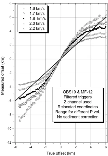
S-wave velocities forF¼0.5 was conducted. The model that provided the best fit between known and estimated ranges had aP-wave velocity of 1.7 km/s and anS-wave velocity of 0.3 km/s. The final fit between estimated and true ranges for the best-fit model had an average error of 273 m but it was less than 50 m at ranges smaller than 3 km (Fig.12). Larger differences still occurred at the larger range offsets and some asymmetry persisted.

The range bias in the estimates obtained for the Lucky Strike dataset is clear but less pronounced [Fig. 12(b)]. Therefore, as for the Gulf of Cadiz, a systematic search of possible models was performed, including an amplitude fac-tor of 0.5. A slight improvement in the average residuals was obtained (135 to 130 m) and the best model was much more realistic, VP¼2.0 km/s, VS¼0.3 km/s, considering the

geo-logical and geophysical characterization of the site. The bias for close ranges completely disappeared (Fig.11).

C. The amplitude factor—a possible cause

The systematic bias in range estimates was seen at two different sites, with two different seismic signals (fin whale calls and airgun shots in the20 Hz range), recorded by two different types of instruments. In both cases, a better fit between estimated and known ranges was obtained by apply-ing an amplitude factor (F¼0.5) to the horizontal channels. An instrumental anomaly does not seem to be an adequate explanation, as the anomaly would have to be shared between two very different sets of instruments. Therefore, a physical explanation is required.

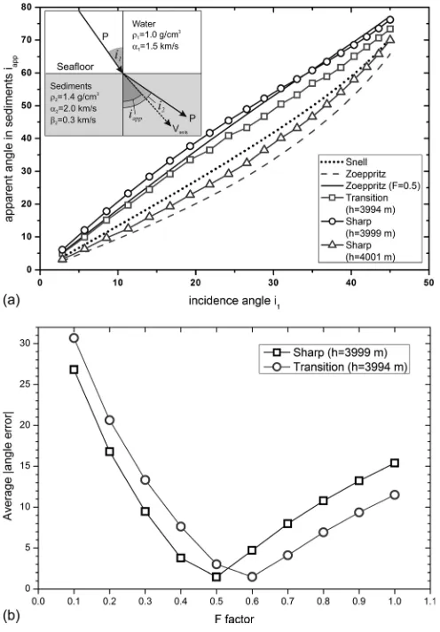
The use of Zoeppritz equations to derive seismic amplitudes is only valid for plane waves propagating with an infinite frequency. Fin whale vocalizations are generated by point sources and constitute bandlimited signals in fre-quency. To verify the results derived by the Zoeppritz equa-tions, seismic amplitudes and apparent angles were obtained by the computation of synthetic seismograms using the seismic reflectivity method as modified byWang (1999). A point source at 20 m depth was considered and a typical fin whale call was used as source wavelet. The velocity model used for the test comprised a water layer of 4000 m above a half space with Vp¼2.0 km/s and Vs¼0.3 km/s. The differences between a very sharp transi-tion between the two domains and a gradual transitransi-tion within a thin layer 10 m thick were also tested. The comparison between the apparent angle obtained for different models as a function of the incident angle at the seafloor is shown in Fig. 13(a). The critical angle for this model is 49.2.

The amplitudes estimated from synthetic seismograms are considerably different from those estimated by the Zoeppritz equations and vary considerably with the position of the sensor in relation to the interface between the two media. When the sensor is just above this interface then synthetic seismograms show that the amplitude ratio between horizontal and vertical signals is considerable changed, as if the horizon-tal amplitudes were amplified. The factor of 0.5 empirically used simply approximates this behavior, particularly at the shorter ranges (i.e., at smaller incidence angles). Comparing the average errors between the synthetic seismogram values and those estimated from the Zoeppritz equations as a function of the amplitude factor, the value of 0.5 is the one that pro-vides the best fit for the sharp transition model and the second best when the transition model is used [Fig. 13(b)]. These results justify the choice of the amplitude factor used in the analysis of the Gulf of Cadiz and Momar site datasets.

V. DISCUSSION

A. Method performance— Detection and classification

The aim of the single station method proposed inHarris

et al. (2013) was to derive reliable range estimates of fin whale calls from OBS recordings that can be used in distance sampling analyses. Given the properties of the interaction between the acoustic waves in the water and the shallowest sediments where the sensor is deployed, the method is lim-ited to a critical distance that depends on the sound speed in the water and P-wave velocity in the sediments. Inside this FIG. 12. Comparison of true and measured offsets for OBS19 recording

critical range the method locates the sound sources close to the surface by measuring the amplitudes of the vertical and horizontal ground velocities and converting these to ranges by considering the water layer stratification and the elastic properties of the sediments (both P- and S-wave seismic velocities). The azimuth of the sound source is also eval-uated so that the relative 2D location of the fin whale can also be obtained. Absolute locations require the knowledge of the seismometer orientation to be inferred from active seismic surveys or passive monitoring of surface waves or body waves (e.g.,Corela, 2014).

In order to be able to use the ranges generated by the method for distance sampling, there are two main criteria that must be met: (1) the measurements of range must be as

accurate as possible and (2) calls produced at zero, or close to zero, horizontal distance from the instrument must be detected with certainty. These are two of the main assump-tions of distance sampling and biased animal density esti-mates can result if these assumptions are violated (Buckland

et al., 2001). Therefore, it was important to confirm that, first, the method could detect fin whale calls inside the criti-cal range and discard all criti-calls generated from sources outside the critical range and all multipath arrivals generated at all ranges. This would ensure that the first assumption was met. It is important to note that false positive detections are rou-tinely dealt with in animal density estimation methods using acoustic data (Marques et al., 2013). However, in this case, false positives caused by calls originating from outside the critical range and multipath arrivals will not only bias the number of observations but also generate false range esti-mates that will affect the estimation of the probability of detection, a key parameter used in distance sampling (Bucklandet al., 2001). Second, it was important to ensure that the algorithm used to identify direct path calls from inside the critical range was not so conservative that direct path calls produced at close horizontal distances to the instrument were rejected. This would ensure that the second assumption was met. Therefore, the detection and classifica-tion process of this single staclassifica-tion method was thoroughly explored in this paper using two control datasets: (i) artificial airgun shots in the Gulf of Cadiz and (ii) fin whale calls recorded in the Azores (at the Lucky Strike area) located by triangulation. Using both datasets, it was verified that the detection procedure, based on a matched filter and a modi-fied normalization of the cross-correlation, was very effec-tive in detecting nearly 100% of the pulses that originated inside the critical range. The most promising classification parameters identified rely on the property that calls originat-ing from outside the critical range cause a phase difference between the four recording channels (the hydrophone, verti-cal, and horizontal channels). This phase difference causes a lag between the hydrophone and vertical channels and degrades the polarization coherency between the three seis-mic channels. The classification procedure was very effec-tive when tested on both datasets. The resulting TPR decayed from one close to the critical range (following the expected reduction in the amplitude of the vertical channel) and was small or null for range offsets larger than the critical range. The FPR considering the number of false triggers in the sequence was estimated and was shown to be small for range offsets larger than the critical range and small to nil within the critical range. Multipaths can have higher ampli-tude than direct paths, which may be problematic, but their amplitude only exceeds the amplitude of primary arrivals at far range offsets (approximately three times the critical range) and also close to the critical range. Therefore, multi-paths could be filtered out by their amplitude or phase differ-ence between channels.

B. Method performance—Ranging

InHarriset al. (2013)the Gulf of Cadiz active seismic survey signals were used to show the reliability of the range FIG. 13. (a) Apparent emergence angle in the sediments computed by

differ-ent methods as function of the incidence angle at the sea-floor. The meaning of the angles and velocity model is shown in the inset.his the sensor depth. The meaning of the functions represented are as follows: Snell, computed by Snell law as if theS-wave velocity in the sediments was null; Zoeppritz, computed using the Zoeppritz equations; Zoeppritz (F¼0.5), computed using the Zoeppritz equations with horizontal amplitudes multiplied by the

estimates generated by the method, assuming some simplify-ing hypotheses. Here the Gulf of Cadiz analysis was expanded by considering the effect of the water layer stratifi-cation and the elastic properties of the sediments. Since the method presented here only applies to small ranges (up to the order of the water depth), the effect of sound propagation in the water was shown to be small but can be corrected using information provided by climatological databases for the water column properties.

As regards the properties of the sediments at the seafloor, they are not known with precision at the sensor locations. For example, the shallowest sediments in the Gulf of Cadiz are thought to consist of soft pelagic sediments with a low

P-wave velocity (1.8 to 2.0 km/s) and a high VP/VS ratio

(Harris et al., 2013). If the S-wave propagation in the sedi-ments is disregarded, then the Snell law applies. This was the simplifying assumption used inHarriset al.(2013). The anal-ysis of the two control datasets showed that if the ideal Zoeppritz equations are applied to the recording of seismic data at the seafloor, then any physically reasonable model for the sediment properties worsens the fit between known and estimated ranges. After a systematic search of parameters, an improvement in the range fit was observed when an empirical factor of 0.5 was applied to the amplitude of the horizontal channels. Using synthetic seismograms, it was verified that the ratio between horizontal and vertical amplitudes recorded at the seafloor by the OBS approximately follows this empiri-cal factor. The amplitude factor appears to be a simple approximation, which can be applied to account for the depar-ture from ideal Zoeppritz equations when the equations are used to estimate the range to a whale call/airgun shot.

C. Conclusions

Data recorded by OBSs, comprising three ground veloc-ity channels and one pressure channel, can be used to iden-tify and locate fin whale vocalizations. The procedure outlined inHarriset al.(2013)and detailed in this work can only be applied to fin whale calls that are direct paths to the sensor and that are incident at the sea-bottom with an angle smaller than the critical incidence that depends on the P -wave velocity in the sediments. To recover the sound source on the surface the method uses the ground velocity ampli-tude measures by the seismometer and corrects the apparent propagation angle taking into account the elastic properties of the sediments. Finally the range and location are derived using the sound speed profile in the water layer. The method also requires that the shallowest seabed properties are esti-mated. In the deep ocean these are of pelagic origin and their properties can be reasonably inferred. However, in very recent oceans, like the Lucky Strike site in the Azores, high porosity and highly fractured volcanic rocks have resulted in low seismic velocities that favor the application of the method. Furthermore, the deeper the OBS, the larger the crit-ical range, within which the method can be applied. This method is then best suited for deep-water deployments on soft sediments or low velocity rocks. Fin whale calls were detected by a matched filter with a modified cross-correlation normalization to reduce the number of detections

to be further analyzed. The master waveform can be extracted from the data itself, selecting one of the strongest calls identified, or it could be a synthetic fin whale call. The method can use a number of classification parameters but the most effective are the ones that use the phase difference between the four channel recordings. These parameters can be used to identify and reject signals generated by post-critical incidence angle at the sea-floor.

ACKNOWLEDGMENTS

The Gulf of Cadiz data were collected for the NEAREST project, on behalf of the EU Specific Programme “Integrating and Strengthening the European Research Area,” Sub-Priority 1.1.6.3, “Global Change and Ecosystems,” Contract No. 037110. The Azores dataset was collected under the MoMAR project and provided to us by Wayne Crawford (Institut de Physique du Globe de Paris). One of the authors contribution (D.H.) was supported by the Office of Naval Research 1172 under the “Cheap DECAF” project, Grant No. 1173 N000141110615. We thank the editor and one anonymous reviewer for their constructive comments, which helped us to improve the manuscript. Publication supported by project FCT UID/GEO/50019/ 2013 - Instituto Dom Luiz.

Aki, K., and Richards, P. (1980). Quantitative Seismology, Theory and Methods(Freeman and Company, San Francisco, CA), Vol. 1, 557 pp. Ambar, I., Serra, N., Neves, F., and Ferreira, T. (2008). “Observations of the

Mediterranean undercurrent and eddies in the Gulf of Cadiz during 2001,” J. Mar. Syst.71, 195–220.

Arnulf, A. F., Singh, S. C., Harding, A. J., Kent, G. M., and Crawford, W. (2011). “Strong seismic heterogeneity in layer 2A near hydrothermal vents at the Mid-Atlantic Ridge,”Geophys. Res. Lett.38, L13320, doi:10.1029/ 2011GL047753.

Arnulf, A. F., Harding, A. J., Singh, S. C., Kent, G. M., and Crawford, W. (2012). “Fine-scale velocity structure of upper oceanic crust from full waveform inversion of downward continued seismic reflection data at the Lucky Strike Volcano, Mid-Atlantic Ridge,” Geophys. Res. Lett. 39, L08303, doi:10.1029/2012GL051064.

Buckingham, M. J. (1998). “Theory of compressional and shear waves in fluid-like marine sediments,”J. Acoust. Soc. Am.103(1), 288–299. Buckland, S. T., Anderson, D. R., Burnham, K. P., Laake, J. L., Borchers,

D. L., and Thomas, L. (2001).Introduction to Distance Sampling(Oxford University Press, Oxford, UK), 432 pp.

Castagna, J. P. (1993). “AVO analysis-tutorial and review,” in Offset-de-pendent Reflectivity—Theory and Practice of AVO Analysis, edited by J. Castagna and M. M. Backus (Society of Exploration Geophysicists, Tulsa, OK), pp. 3–37.

Chauhan, A., Rai, A., Singh, S. C., Crawford, W. C., Escartin, J., and Cannat, M. (2009). “OBS records of whale vocalizations from Lucky-Strike segment of the Mid-Atlantic Ridge during 2007–2008,” in

Proceedings of the American Geophysical Union, Fall Meeting, San Francisco, CA, abstract #S51D-07.

Corela, C. (2014). “Ocean bottom seismic noise: Application for the crust knowledge, interaction ocean-atmosphere and instrumental behaviour,” Ph.D. thesis, University of Lisbon, 339 pp.

Crawford, W. (2013). (personal communication).

Crawford, W. C., Beguery, L., Daniel, R., Corela, C., Duarte, J. L., Hananto, N., Cordeiro, A., Pasquet, S., and Arnulf, A. (2008). BBMOMAR-2 cruise report, IPGP, 47 pp.

Crawford, W. C., Rai, A., Singh, S. C., Cannat, M., Javier Escartin, J., Haiyang Wang, H., Romuald, D. R., and Combier, V. (2013). “Hydrothermal seismicity beneath the summit of Lucky Strike volcano, Mid-Atlantic Ridge,”Earth Planetary Sci. Lett.373, 118–128.

Favretto-Cristini, N., Cristini, P., and de Bazelaire, E. (2007). “Influence of the interface Fresnel zone on the reflected P-wave amplitude modelling,” Geophys. J. Int.171(2), 841–846.

Hamilton, E. (1976). “Shear wave velocity versus depth in marine sedi-ments: A review,”Geophys.41(5), 985–996.

Harris, D., Matias, L., Thomas, L., Harwood, J., and Geissler, W. H. (2013). “Applying distance sampling to fin whale calls recorded by single seismic instruments in the Northeast Atlantic,”J. Acoust. Soc. Am.134, 3522–3535. Kasahara, J., Nagumo, S., Koresawa, S., Daikuhara, T., and Miyata, H. (1980). “Experimental results of vortex generation around ocean bottom seismograph due to bottom current,” Bull. Earthquake Res. Inst., Univ. Tokyo55, 169–182.

Lobue, N. (2012). (personal communication).

Marques, T. A., Thomas, L., Martin, S. W., Mellinger, D. K., Ward, J. A., Moretti, D. J., Harris, D., and Tyack, P. L. (2013). “Estimating animal population density using passive acoustics,”Biol. Rev.88(2), 287–309. McDonald, M. A., Hildebrand, J. A., and Webb, S. C. (1995). “Blue and fin

whales observed on a seafloor array in the Northeast Pacific,”J. Acoust. Soc. Am.98(2), 712–721.

Nafe, V. E., and Drake, C. L. (1963). “Physical properties of marine sed-iments,” inThe Sea, edited by M. N. Hill (Interscience, New York), Vol. 3, pp. 794–815.

NEAREST—Integrated Observations from Near Shore Sources of Tsunamis: Towards an Early Warning System (2012). http://nearest.bo. ismar.cnr.it(Last viewed March 16, 2014).

Nieukirk, S. L., Mellinger, D. K., Moore, S. E., Klinck, K., Dziak, R. P., and Goslin, J. (2012). “Sounds from airguns and fin whales recorded in the mid-Atlantic Ocean, 1999–2009,” J. Acoust. Soc. Am. 131(2), 1102–1112.

Ottem€oller, L., Voss, P., and Havskov, J. (2011). SEISAN: Earthquake anal-ysis software for Windows, Solaris, Linux and Mac OSX, 361 pp. Payne, R., and Webb, D. (1971). “Orientation by means of long range

acous-tic signaling in baleen whales,”Ann. N.Y. Acad. Sci.188, 110–141. Rebull, O. G., Cusı, J. D., Fernandez, M. R., and Muset, J. G. (2006).

“Tracking fin whale calls offshore the Galicia Margin, north east Atlantic ocean,”J. Acoust. Soc. Am.120(4), 2077–2085.

Roberts. R. G., Christoffersson, A., and Cassidy, F. (1989). “Real time events detection, phase identification and source location estimation using single station component seismic data and a small PC,”Geophys. J.97, 471–480. Seher, T., Singh, S. C., Crawford, W. C., and Escartın, J. (2010). “Upper crustal

velocity structure beneath the central Lucky Strike Segment from seismic

refraction measurements,”Geochem. Geophys. Geosyst.11, Q05001, doi: 10.1029/2009gc002894.

Shipboard Scientific Party (1972). “Sites 135,” inInitial Reports of the Deep Sea Drilling Project, Vol. 14, edited by D. E. Hayes, A. C. Pimm, J. P. Beckmann, W. E. Benson, W. H. Berger, P. H. Roth, P. R. Supko, and U. von Rad (U.S. Government Printing Office, Washington, DC), pp. 15–48.

Sirovic´, A., Hildebrand, J. A., and Wiggins, S. M. (2007). “Blue and fin whale call source levels and propagation range in the Southern Ocean,” J. Acoust. Soc. Am.122(2), 1208–1215.

Somoza, L., Anahnah, F., Bohoyo, F., Gonzalez, J., Hernandez, J., Iliev, I., Leon, R., Llave, E., Maduro, C., Martınez, S., Perez, L. F., and Vazquez, T. (2007). “Informe cientıfico-tecnico, N/O L’ATALANTE” (“Scientific and technical report, R/V L’Atalante”), August 23 to September 9, 2007, project report, http://tierra.rediris.es/GulfofCadiz/GulfofCadiz_informe_final.pdf (Last viewed July 25, 2014).

Stafford, K. M., Citta, J. J., Moore, S. E., Daher, M. A., and George, J. E. (2009). “Environmental correlates of blue and fin whale call detections in the North Pacific Ocean from 1997 to 2002,”Mar. Ecol. Prog. Ser.395, 37–53.

Thompson, P. O., Findley, L. T., and Vidal, O. (1992). “20-Hz pulses and other vocalizations of fin whales,Balaenoptera physalus, in the Gulf of California, Mexico,”J. Acoust. Soc. Am.92, 3051–3057.

Wang, R. (1999). “A simple orthonormalization method for stable and effi-cient computation of Green’s functions,” Bull. Seis. Soc. Am. 89(3), 733–741.

Watkins, W. A., Tyack, P., Moore, K. E., and Bird, J. E. (1987). “The 20-Hz signals of finback whales (Balaenoptera physalus),”J. Acoust. Soc. Am. 82, 1901–1912.

Webb, S. C. (1998). “Broadband seismology and noise under the ocean,” Rev. Geophys.36(1), 105–142, doi:10.1029/97RG02287.

Weirathmueller, M., and Wilcock, W. S. D. (2013). “An automatic single station multipath ranging technique for 20 Hz fin whale calls: Applications for ocean bottom seismometer data in the northeast Pacific,” J. Acoust. Soc. Am.134, 4147.

Weirathmueller, M., Wilcock, W. S. D., and Soule, D. C. (2013). “Source levels of fin whale 20 Hz pulses measured in the Northeast Pacific Ocean,”J. Acoust. Soc. Am.133, 741–749.