Impact of land cover patch size on the accuracy of patch area representation in HNN based super resolution mapping

Impact of land cover patch size on the accuracy of patch area representation in HNN-based super resolution mapping.

Muad, A. M. and Foody, G. M.

IEEE Journal of Selected Topics in Applied Earth Observations and Remote Sensing

, 5, 1418-1427 (2012).

The manuscript of the above article revised after peer review and submitted to the

journal for publication, follows. Please note that small changes may have been made

after submission and the definitive version is that subsequently published as:

Muad, A. M. and Foody, G. M., 2012, Impact of land cover patch size on the accuracy of patch

area representation in HNN-based super resolution mapping,

IEEE Journal of Selected

Impact of land cover patch size on the accuracy of patch area representation in HNN-based super resolution mapping.

Anuar M. Muad1 and Giles M. Foody2

1. Department of Electrical, Electronic and Systems Engineering, Universiti Kebangsaan Malaysia, 43600 UKM Bangi, Selangor, Malaysia (e-mail: [email protected])

2. School of Geography, University of Nottingham, Nottingham, NG7 2RD, UK (e-mail [email protected])

Abstract

Mixed pixels are one of the largest sources of error and uncertainty in mapping from remotely sensed

data. A Hopfield neural network based approach to super-resolution mapping has become popular for

mapping at a sub-pixel scale, partly because it seeks to maintain the class proportional information

indicated by a soft classification analysis. The use of the approach is, however, handicapped by a lack

of guidance on the parameter setting values and of the impacts of different landscape patterns on the

analysis. Here, the sensitivity of the Hopfield neural network for super-resolution mapping is

investigated with a focus on the effect of different landscape types and parameter settings using

simulated and real data sets. It is shown that the method‟s suitability varies between landscapes, being

most suited to situations in which landscape patches are large (>1 pixel). Additionally, for such

landscapes the widely used scenario in which the weighting parameters are set at equal values is

successful but the approach is less effective for the mapping of small isolated land cover patches.

With the latter, it is shown to be important to weight the area constraint highly and undertake a large

number of iterations. Critically, it is shown that equal weighted parameter settings and imbalanced

settings to emphasise the area constraint are most suitable for landscapes comprising large and small

patches respectively. Moreover, the positive attributes of these two sets of parameter settings may be

combined to yield an enhanced mapping method for landscapes that comprise a mixture of patch

I. Introduction

Mixed pixels are one of the major sources of error and uncertainty in the mapping of land cover from

remotely sensed data [1]. Given that a mixed pixel must by definition represent an area containing two

or more land cover classes, such pixels cannot be appropriately represented by conventional „hard‟

image classifications used widely to map land cover [2-4]. Unmixing and soft classification methods

that allow for the multiple and partial class membership properties of mixed pixels have proved

popular for mapping from remotely sensed imagery. They have been used in a range of studies,

including those representing gradations between continuous classes [5,6] and those estimating the

class composition of pixels [7,8] as well as forming the basis of important land cover data products

such as vegetation continuous fields [9,10]. Although representing a major advancement on the

conventional hard classification, the output of a soft classifier and its interpretation can be

problematic. The output is, for example, typically a set of fraction images, each depicting the

proportional cover of one of the classes in the area represented by the pixel which is harder to

interpret than the standard, single layer, thematic map derived by a hard classification. Additionally,

the soft classification only indicates the class composition of image pixels, it does not indicate the

geographical distribution of the classes in the area represented by the pixels [11]. One means to

address these concerns and produce a single layer land cover map which shows the spatial distribution

of the classes at a finer resolution than the image is to apply a super resolution mapping technique to

the output of a soft classification.

A variety of super resolution mapping methods has been used in remote sensing [11-18].One that has

been widely promoted and demonstrates considerable potential is based on the Hopfield neural

network (HNN) [19-21]. A key feature of the HNN is that it seeks to maintain the class proportional

information of the soft classification in the super resolution map. Thus, the estimated proportion of a

pixel‟s area comprised of a class depicted in a soft classification, or a value close to it, should also be

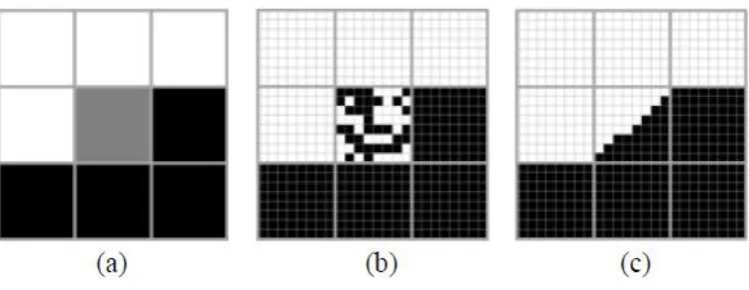
With the HNN based approach to super-resolution mapping, a pixel is decomposed into a large

number of sub-pixels and the class labels of these sub-pixels are distributed in proportion to the class

composition information provided by a soft classification for the pixel. The labels are initially

distributed randomly amongst the sub-pixels and the HNN estimates their spatial distribution through

an iterative analysis. The latter involves adjusting the sub-pixel class labels on the basis of the class

label information for a sub-pixel and its immediate neighbourhood. As the approach incorporates

spatial context into the determination of the location of sub-pixel class fractions the method is most

suitable for the scenario in which the land cover patches are relatively large relation to the image pixel

size. This type of scenario is common, with mixed pixels occurring at the edge of patches. There is,

however, a variety of land cover mixing scenarios [22] and the basic HNN approach may not always

be appropriate for the representation of the land cover distribution. In particular, one concern is when

the mixing arises because of the landscape mosaic comprises small (area <1 pixel) isolated land cover

patches. This may be a common occurrence, with the amount of small land cover patches varying as

an interactive function of patch size relative to image spatial resolution.

This article aims to evaluate the effect of land cover patch size on the accuracy of super resolution

mapping by a HNN with particular regard to the accuracy with which patch area is represented.

Section II provides a review of the key features of the HNN algorithm used for super resolution

mapping. The data and methods used are described in Section III. Section IV provides the results and

section V the conclusions.

II. HNN

The HNN is a recurrent artificial neural network which is designed for the solution of optimization

problems [23, 24]. The fundamental structure of the network consists of a single layer of neurons and

the output of each neuron is fed back to all other neurons except itself. The HNN is an optimization

tool defined by an energy function [24] formulated for the application. In super-resolution mapping

sub-pixels, where z is the zoom or scale factor of the spatial resolution increment. Each sub-pixel is

associated with a single neuron in the HNN and can be located by its coordinates in the sub-pixel grid.

The input to the neuron at row i column j of the grid is uij and its output is vij.

The energy function that represents the problem of super-resolution mapping is generally represented

as the sum of a goal and constraint term. The goal function considers the spatial correlation between

observations, working on a neuron together with its closest neighbours rather than treating each

neuron as an independent unit. The constraints specify the context of the available data by adding

costs to the objective. By assuming that the spatial dependence between a neuron and its adjacent

neurons is larger than that of neurons that are more distant, the energy function can be represented as

the combination of spatial clustering goal functions and an area proportion constraint [19, 20, 25]

which can be expressed as





ON OFF

ij ij P ij

i j

E 



where E is the network energy,

G

G

 

i j

,

P

proportion constraint, k1, k2, and kP are the weight constant for the goal functions and the area proportion constraint respectively. The rate of change for the energy function for a neuron is

1 2

ON OFF

ij ij ij ij

P

ij ij ij ij

dE

dG

dG

dP

k

k

k

dv



dv



dv



dv

The goal functions maximize the spatial correlation of nearby neurons that have similar values. The

functions receive input from the neuron and its eight surrounding neurons. Two goal functions are

used to drive the output into two binary states: on and off. The first goal function,

G

output of a neuron to 1 if the average value of its eight surrounding neurons is greater than a threshold

function becomes 0. This function makes the output of a neuron similar to that of its neighbouring

neurons and is based on





1 1

1 1

1

1

1 tanh

1

2

8

ON i j

ij

kl ij

k i l j ij

k i l j

dG

v

T

v

dv





















_



_



_

_











_

_







 

where λ is the gain that determines the steepness of the tanh function. The second goal

function,

G

neurons is less than T. If the average of the surrounding neurons is greater than T, the second function

increases the output of the centre neuron to 1. Again, this function makes the output of a neuron

similar to that of its neighbouring neurons and is based on

1 1 1 1

1

1

1 tanh

2

8

OFF i j

ij

kl ij

k i l j ij

k i l j

dG

v

T

v

dv





















_



_



_

_



















 

The area proportion constraint regulates the energy equation by seeking to retain the pixel class

proportion derived from soft classification, which for a pixel at location (x,y) in the image‟s pixel grid

is denoted

a









1

1 tanh

2

m xz n yz ij

dP

v

T

a

dv

z



   

 







_





_





 



If the area proportion of the estimate for the original pixel is lower or greater than the target area, the

output values of the neurons are increased or decreased accordingly to help address the problem [19,

25]. The value for each neuron in the HNN can be updated numerically using a Euler method [26] and





 

 

ij ij

du t

u t t u t t

dt

     (6)

which advances a solution from state

u t

 

u t



 

t





t

Equation 6 runs iteratively until







 



u t  t u t 







Operational use of the HNN approach to super-resolution mapping requires the analyst to specify the

values of the weight parameters in equation 1 and the number of iterations to undertake or value for



to act as a stopping criterion. The selection of optimum parameter settings can be a difficult and

tedious process and the literature provides little guidance on the settings to use. It is common, for

example, for weighting parameters to be set at equal values and to use >2000 iterations [19, 25]. The

settings used are often selected on the basis of assumptions made by the analyst and trial runs [19,

21]. A strategy to enhance the analysis is also to include prior information on the land cover mosaic, if

known, perhaps via a semi-variance function [21] and/or provision of ancillary data [27, 28]. The

inclusion of prior information in terms of a semi-variance function is, for example, one means to

enhance the utility of the HNN for the representation of small land cover patches. To achieve this, the

basic approach represented by equation 1 is adjusted such that the energy function is represented as

the sum of a set of semi-variance functions and an area proportion constraint [21] which, assuming a

zoom of z, can be expressed as

     





1 2

z

ij ij z ij P ij

i j

E  



where

k

to

k

are weighting factors for the output values for

z

semi-variance function,

S

to

 z ij

S

. As explained by [21] the rate of change for the energy function becomes

 

1

n z

ij ij ij

n P

n

ij ij ij

dE dS dP

k k

dv  dv dv

 

_ _





in which the first part corresponds to the semi-variance functions while the second part is for

the area proportion constraint. The prior knowledge about spatial pattern, perhaps from a fine

spatial resolution image, is modelled using a semi-variance function

 

_{ }





, 1, 1

1

2

N h

ij i h j h

i j

h

f

f

N h



 







in which



 

h

is the semi-variance at lag

h

,

N

(

h

) is the number of pixels at lag

h

from the

centre pixel (

i

,

j

) and

f

is a pixel of the fine spatial resolution image used to generate the prior

information. Further details on the approach are given in [21].

III. Data and Methods

A variety of real and simulated data sets were used and discussed in four groupings.

A. Fine resolution imagery

To illustrate the sensitivity of the HNN to different mixing scenarios a set of four small images

representing similar land covers but present in different patterns was derived from a SPOT image

contained in Google Earth for a site near Granada, Spain. Each image extract was derived from a

region lying between latitudes 37° 08' 19"N and 37° 07' 41"N and longitudes 4° 07' 60"W and 4° 07'

09"W from an image acquired on 1 October 2004. The agricultural land use of the site produced four

visually different landscape patterns, A-D (Figure 1) each comprised of two classes: vegetation and its

background. Each image was spatially degraded by a factor of 8 with the pixels in the derived

simulated coarse resolution images taking on the average value of the pixels in an 8×8 area of the

original image. These simulated coarse resolution images were subjected to a series of analyses, using

a standard k-means hard classification and super-resolution mapping by HNN using a zoom factor of

8 to predict the land cover distribution. The number of cluster in the k-means classifier was set to two

to differentiate between the vegetation and its background. The input to the HNN analyses was a soft

classifier in which the weighting parameter that determines the degree of fuzziness was set to 2.0.

Following common practice, the weights in the HNN were set to equal values: k1=k2=kp=1. A further analysis was undertaken with the HNN informed by information on the land cover pattern represented

by the semi-variogram [21] derived from each of the original resolution images.

Accuracy assessment is typically based on the comparison of the derived land cover representation

against a high quality reference. As a gold-standard reference data set is typically unavailable, this

process often involves the evaluation of the degree of agreement between the derived representation

and another, high quality, classification used as a reference [1]. Here, the accuracy of each analysis

was evaluated against a standard hard classification of the relevant original fine resolution imagery

(Figure 1c). The latter reference data were derived by a k-means classification of the original imagery.

The degree of correspondence between the predicted and ground reference land cover distributions

was evaluated visually and by cross-tabulation of the pixel labels, at a sub-pixel scale, with accuracy

expressed as the percentage overall agreement in labelling. Although there are concerns with the use

of site-specific accuracy assessment in the evaluation of super-resolution maps [30] the focus here is

on the relative rather absolute magnitude of the estimates derived.

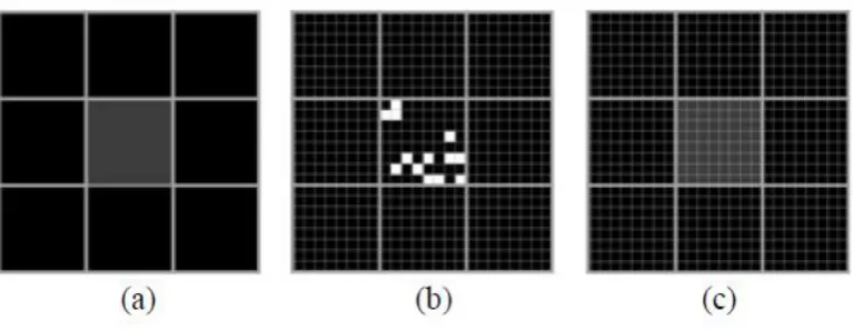
B. Simulated blocks of pixels

The relationship between land cover patch size and its predicted area was explored with simulated

data representing blocks of image pixels. As with the previous example, the focus was on a simple

situation in which there are just two classes; the patch and its background. Initial analyses focused on

the representation of a relatively large patch and a small isolated patch by the standard HNN. This

situation was evaluated with simulated data comprising blocks of 3×3 pixels in a coarse spatial

resolution image. Two sets of scenarios were evaluated. The first was for the situation when the land

cover patches were relatively large and information from neighbouring pixels could usefully inform

the HNN analysis and the soft classification value of the central pixel was varied from 0.05 to 1.0

with all values at a 0.05 step evaluated. The second set of scenarios was similar but with the land

block contains a single small patch of one land cover class with the rest of the 3×3 pixel area

representing the background class. Again the soft classification value of the central pixel was varied

over the range 0.05 to 1.0. In each case it was assumed that the soft classification of the data was

perfect, and so the DN or value for a pixel in the soft classified image corresponded to the

proportional cover of the class in the area represented by that pixel.

Three different HNNs were evaluated. First, the weighting parameters were set at equal values.

Specifically, the k1=k2=kp=1 scenario was again used and as the parameters were of equal magnitude this is approach is referred to as HNN(E). Second, a HNN with the goal function parameters set at a

higher level than the area proportion constraint. This latter analysis used k1=k2=1.0 and kp=0.1 and as the goal functions were emphasised is referred to as HNN(G). Thirdly, a scenario in which the area

proportion constraint was emphasised over the goal functions. With this scenario k1=k2=0.1 and kp=1.0 and as the area proportion constraint was emphasised it is referred to as HNN(A). Analyses with these

three HNNs were undertaken over a range of iterations: 1,000, 2,000, 5,000, 10,000 and 15,000.

To further explore the effects of different weight parameter settings, the HNN(G) approach was also

modified to explore the effect of variation in the kp value. For this, k1=k2=1.0 throughout but the value

of kp was altered in 0.1 increments over the range 0.1 to 1.0. Similarly, with the HNN(A) approach a series of analyses were undertaken in which kp was fixed at 1.0 throughout but the value for k1=k2 was

varied over the range 0.1 to 1.0 with a 0.1 step.

C. Simulated imagery

Variation in the representation of patch area was expected, mainly because the relative weighting of

the area proportion constraint in the various analyses. It was anticipated that the accuracy of patch

representation derived with the data outlined in section B above would vary between the three HNN

scenarios as a function of patch size. However, it was also anticipated that the strengths of different

approaches could be exploited and combined to form an enhanced analysis. To assess this, an image

patches was determined in an unplanned, haphazard, manner. As with other analyses, this image was

degraded by a factor of 8 and a soft classification of the resulting coarse resolution image derived by

the FCM with the weighting parameter set to 2.0. The soft classification was used as input to the

HNN(E) and HNN(A). The outputs of these HNNs were also combined. This was achieved by using

the output of HNN(E) for the large patches (defined here as >1 pixel in area) and HNN(A) for the

remaining, small, patches. Since the approach is a combination of two HNN scenarios this is referred

to later as the HNN2.

The area of the patch in the output of each HNN analysis was calculated by counting the number of

sub-pixels allocated to the patch class. This value could be compared directly against the actual

proportion of patch cover, which was known from the simulation. Attention focused on the accuracy

of the estimation over a range of patch sizes, expressed in terms of the patch proportional cover,

which is illustrated in plots of the predicted against actual cover. In these plots deviation from the 1:1

line indicates error, with values lying below the line highlighting an underestimation of patch area.

D. Coarse resolution imagery

Finally, a series of analyses of remote sensor data sets were undertaken to illustrate the issues in a real

application. As in other studies, the adoption of finer spatial resolution imagery can enhance spatial

detail and provide accurate information [31, 32]. Here, the focus was on the mapping of high latitude

lakes from MODIS imagery. Presently there is considerable uncertainty over the number and size of

lakes [33], especially at high latitudes where they may be disappearing due to climate change [34].

Mapping and monitoring lakes over such large regions is realistically only feasible with moderate

spatial resolution systems such as MODIS, but the spatial resolution makes it difficult to study small

lakes, which are often of interest as associated with considerable uncertainty [33]. Here, the potential

of HNN based super-resolution mapping for the provision of information on lakes was evaluated. This

work mapped lakes from MODIS data for a test site in Quebec province of Canada (Figure 3)

acquired on 5 July 2002. As attention was focused on mapping water, which is relatively separable

resolution image in the near infrared (841-876 nm) waveband was used. The MODIS imagery used

was derived from tile 13 horizontal and 03 vertical of the MOD09GQ, a level 2 data, which have not

been gridded into a map projection as in Level 3 data of composite images [35], facilitating further

processing to be determined by users, such as relative shift measurement and reduction of sensor point

spread function effects [36]. The MODIS images were projected from Sinusoidal projection into a

Landsat Universal Transverse Mercator (UTM) projection at zone 16.

A Landsat ETM+ image with a 30m spatial resolution acquired five days after the MODIS image on

10 July 2002 was also obtained. The image used was acquired on path 25 row 22 and obtained from

the US Geological Survey. A k-means hard classification of the ETM+ data acquired in the

near-infrared waveband (770-900nm) was used as reference data for the evaluation of the analyses of the

MODIS data. The latter analyses included a standard k-means hard classification and super-resolution

mapping using the HNN(E) and HNN(A), both with z=8 and run for 10,000 iterations. Note that the

settings of the HNN analyses yield a map with a spatial resolution of ~31.2 m, approximately the

same as the ETM+ data used as reference data. As previously, the FCM with a weighting parameter of

2.0 was used to generate a soft classification for input to the HNN.

IV. Results and Discussion

A. Fine resolution imagery

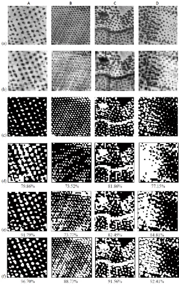
The four landscape mosaics, A-D (Figure 1), were represented with varying quality by the k-means

hard classification and HNN analyses. For each landscape, the hard classification provided the least

accurate representation which was also unrealistic visually due to its blocky nature (Figure 1d). The

hard classification was particularly poor in representing mosaic B, with many of the very small,

sub-pixel sized, patches not represented in the classified image. The accuracy with which the four

landscapes were mapped by the hard classification ranged from 73.52% to 81.86%

The super-resolution maps were all more accurate than the hard classification for each landscape type

For example, with the basic HNN (figure 1e), landscape A was classified to a very high accuracy, and

substantially higher than the representation derived for that landscape in the hard classification. For

landscape B, however, the HNN was only marginally (0.25%) more accurate than that observed with

the hard classification. The accuracy of the HNN derived maps varied from 73.77% to 91.79%, a

range of 18.02%, a result which highlights that the utility of the HNN for super-resolution mapping

varies as a function of the landscape mosaic to be represented.

The addition of prior information into the HNN analysis increased the accuracy of the land cover

representations for all four landscapes. Accuracy varied from 88.73% for landscape B to 96.70% for

landscape A, a range of 7.97% (Figure 1f). The acquisition of suitable prior information may,

however, be difficult. Furthermore, it is important that the prior information used is suitable. Figure 4

illustrates the effect of using an inappropriate prior on the analysis, with the output over-influenced by

the prior.

The analyses of the four landscapes (Figure 1) highlight the value of super-resolution mapping over

conventional hard classification. More critically, they also show that the HNN based approach varies

in suitability over the four landscapes, being most suitable when the patches were relatively large (e.g.

landscape A) and least where the patches were small (e.g. landscape B). The impact of variation in

patch size on the HNN was explored further with the simulated data.

B. Simulated blocks of pixels

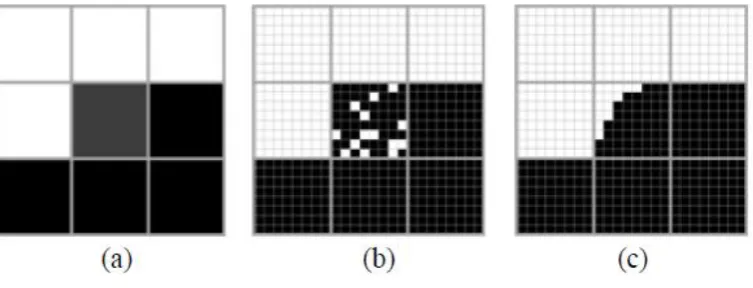
The impact of land cover patch size on the super-resolution representation is illustrated in Figures 5-8.

For large patches, the basic HNN approach produced a visually realistic representation of the

geographical distribution of the classes. In Figures 5 and 6 it is evident how information from

neighbouring pixels aided the location of the patch cover in the central pixel. However, for small

patches, which are associated with a low value in the soft classification and surrounded by other low

or zero values, the HNN can produce a reasonable representation if the patch is relatively large

the soft classification value of a pixel and its neighbours on the prediction of land cover distribution

by HNN.

In the basic HNN approach the algorithm‟s parameters had, as is common practice, been set at equal

values (k1=k2=kp=1). Varying the parameter values may be one means to enhance the representation, especially of the small patches that have been shown above to be problematic in super-resolution

mapping by HNN.

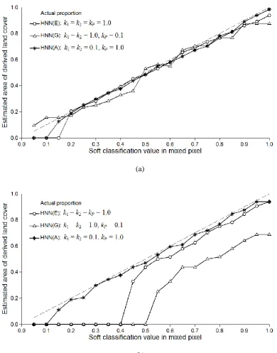
Using the HNN(E), HNN(G) and HNN(A), the analyses reported above were repeated but across the

full range of soft classification values. For large land cover patches each of the three HNN scenarios

provided accurate representations of the patch area, with predictions lying close to the 1:1 line in

Figure 9a. Differences between the scenarios were small but most apparent at low soft classification

values. The results indicated that the minimum soft classification value, and so patch size, required for

a patch to be represented in the output was 0.05 for HNN(G), 0.15 for HNN(A) and 0.20 for HNN(E);

the estimated size of these patches were close to the 1:1 line across the full range of soft classification

values above the minimum patch size noted.

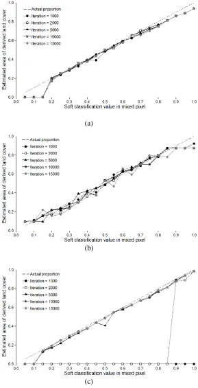
For the small patches, however, it was evident that the accuracy with which patch size was estimated

by all three HNN scenarios varied greatly with the soft classification value and hence patch size

(Figure 9b). It was especially evident that while HNN(A) consistently underestimated patch size the

estimates derived were close to the actual value, lying close to the 1:1 line. However, the results from

the HNN(E) and, especially, HNN(G) were less accurate. For the HNN(E) patch size was again

consistently underestimated but generally close to the 1:1 line for soft classification values >0.5. At a

soft classification value <0.5 the underestimation was large and a patch was not represented at all at

values of 0.4 and below. The HNN(G) provided the least accurate results for small patches. Again,

patch size was consistently underestimated, deviating considerably from the 1:1 line across the entire

range of soft classification values. Additionally, a patch associated with a soft classification value of

the HNN(A) was able to provide accurate predictions of patch size across the entire range of soft

classification values, helping to address concerns highlighted in relation to Figure 8. The HNN(E)

and HNN(G) were less useful, especially for the smallest patches.

As well as the values of the k1, k2 and kp weighting parameters, the number of iterations can have an impact on super-resolution mapping by a HNN. Variation in the number of iterations had little effect

on the representation of the large land cover patches by the three HNN scenarios except for the

HNN(A) (Figure 10). With the latter, it was evident that at a small number of iterations, 2000 or less,

poor estimates of patch size were derived. For large land cover patches the HNN(E) and HNN(G)

could be used to derive accurate estimates with a small number of iterations. A larger number of

iterations, here ~5000 or more, was required for accurate estimation with the HNN(A).

For the small land cover patches the number of iterations had little impact on the accuracy of the

estimates derived from the HNN(E) and HNN(G) but a large effect on the results from the HNN(A)

(Figure 11). With the latter, the estimates derived from the use of 2000 and especially 1000 iterations

were substantially underestimated. However, with a large number of iterations, the accuracy was high

with estimates lying close to the 1:1 line (Figure 11). This is further emphasised in the visualization in

Figure 12 of the results for one of the analyses, based on the situation when the value of the pixel in

the soft classification was 0.2, which shows the requirement for a large number of iterations. The

results above highlight the potential of the HNN(A) for the representation of small land cover patches,

especially when a relatively large number of iterations is used.

As the weight parameter settings used in the scenarios were defined relatively arbitrarily, it is

interesting to note results obtained from different settings as this could influence the performance of

the HNN(G) and HNN(A) methods. With the HNN(G) it was apparent that with k1=k2=1 variation in

k2. In particular, when the soft classification value was low a small value for k1 and k2 was preferable

(Figure 14).

The results indicate that HNN(E) is suited to the situation when the patches are large, larger than a

pixel. For patches smaller than the size of the pixel, the HNN(A) was most suitable, especially if low

values were used for k1 and k2 and large number of iterations undertaken.

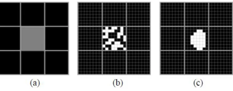
C. Simulated imagery

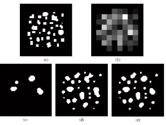
Application of the HNN(E) and HNN(A) approaches to a simulated image containing a variety of

patches of differing size helps illustrate their potential and limitations for super-resolution mapping.

Of the 34 patches present (figure 2a), the HNN(E) was able to represent only 4 large patches (Figure

2c). Alternatively, the HNN(A) was more suited to the task as most patches were small and isolated

and so it was able to represent 24 of the patches (Figure 2d); the 10 patches it missed were typically

very small. However, it was evident that the representation of the large patches by the HNN(A) was

often poor, with size and shape visually incorrect (Figure 2d).

The results highlight that the HNN(E) may be expected to work well for large patches while the

HNN(A) appears most suitable for the representation of small patches. In many landscapes there may

be a mixture of patch sizes and neither approach would be ideal. The proposed HNN2 approach,

which seeks to use the positive aspects of each method by gaining information on the large patches

from the HNN(E) and the small patches from HNN(A) provided a better representation than the two

HNNs it was based on. It too yielded a representation of 24 patches (Figure 2e) but visually this was

superior to that from both the HNN(E) and HNN(A).

D. Coarse resolution imagery

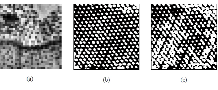
Similar trends were also observed in the analyses based on the MODIS data. The test site contained a

wide variety of lakes, differing greatly in terms of size and shape. Critically, some of the lakes were

were small and isolated and not suited to standard HNN analyses. A visual analysis illustrates the

quality of the mapping by standard hard classification and HNN based methods (Figure 15). The hard

classification of the MODIS data yielded a representation in which the lake boundaries were

unrealistically jagged and clearly omitted the numerous small lakes (Figure 15b). The soft

classification of the MODIS image yielded an enhanced representation (Figure 15c), with information

on the small lakes more apparent. However, the three HNN analyses based on the soft classification

provided representations that were much closer to the reference data than the standard hard

classification. As noted above, the reference data set was a k-means classification of the Landsat

ETM+ data. While it is not feasible to provide a rigorous evaluation of the accuracy of the k-means

classification and so its suitability as a reference, a guide to its quality was obtained by checking its

labelling against visual interpretation of the Landsat ETM+ image. The latter indicated that the k

-means classification had an accuracy of 90.5% and so provides a strong, albeit imperfect, reference

data set.

It was evident that the HNN(E) appeared to provide an accurate representation of the large lakes, with

small lakes omitted (Figure 15d). The HNN(A) and HNN2, however, provided representations that

depicted a greater number and variety of lakes (Figure 15e, 15f). While not suited to site-specific

accuracy assessment because the precise location of a small patch is uncertain [30], non-site specific

accuracy assessment highlighted some important trends. The reference data indicated that the total

extent of lake water in the region was 202.09 km2, with much of this area associated with small, often

very small, lakes. The HNN(E) which omitted small lakes provided a representation with 151.89 km2

while the HNN(A) and HNN2 were closer with 161.94 km2 and 162.89 km2. Although there was little

difference between the HNN(A) and HNN2 in terms of the areal extent estimates, it was apparent that

the shape of the lakes appeared to be more accurately represented by the HNN2. Further work to

validate these and other super-resolution products would be useful but needs to address concerns

V. Conclusions

The HNN has been widely used in super-resolution mapping applications. One attraction of the

approach is that it includes a parameter that seeks to maintain the class proportional information

provided by the soft classification upon which the analysis is based. There is, however, little guidance

in the literature on what weight settings to use and the suitability of the HNN for different types of

landscape. Here, the effect of different parameter settings and landscape patterns on HNN analysis

was evaluated. There are five main conclusions to this work:

1. The suitability of the HNN for super-resolution mapping varies as a function of the landscape

to be represented. The basic HNN approach with equally weighted parameters, HNN(E), was

able to provide accurate representations when patches were large but not when small. For

example, the accuracy with which a landscape comprising relatively large patches was

increased from 79.86% with a hard classification to 91.79% with the HNN(E). However, for a

landscape composed of small patches the accuracy of the representation derived from a hard

classification and HNN(E) analysis were very similar, at 73.52% and 73.77% respectively.

2. The incorporation of prior information into the HNN analysis could increase the accuracy of

the mapping for each landscape pattern but it was essential that an appropriate prior was used.

3. When patches were relatively large, all three HNN scenarios investigated were able to derive

highly accurate land cover representations. Additionally, the number of iterations had little

effect on the results of the HNN mapping except for the HNN(A) which yielded most

accurate representations when a large number of iterations was used.

4. When patches were relatively small, the HNNs using equally weighted and goal emphasised

parameter settings tended to underestimate patch area, especially for the very small patches.

By emphasising the area proportion constraint, as in HNN(A), the accuracy with which small

patches could be represented was increased, especially if a large number of iterations was

employed. Critically, the popular use of equal parameter values in the HNN(E) yielded

substantial under-estimation of patch area when patch size was <0.5 pixel area.

5. When the region to be mapped contains a variety of patch sizes, both large and small, neither

to represent large patches and combined with that from HNN(A) for small patches to derive

an enhanced representation.

Acknowledgments

We are grateful for the data sets used: the MODIS data from the USGS Land Processes Distributed

Active Archive Center (https://lpdaac.usgs.gov/), the Landsat data from the USGS global

visualization viewer (http://glovis.usgs.gov/) and Google Earth. We are also grateful to the Ministry of Higher Education of Malaysia and the Universiti Kebangsaan Malaysia for sponsoring AMM‟s

research for a PhD degree at the University of Nottingham as well as the constructive review

comments from the editors and three referees.

References

1. G. M. Foody, “Status of land cover classification accuracy assessment,” Remote Sensing of

Environment,” vol. 80, pp. 185-201, 2002.

2. P. F. Fisher and S. Pathirana, “The evaluation of fuzzy membership of land cover classes in

the suburban zone”, Remote Sensing of Environment, vol. 34, pp. 121-132, 1990.

3. G. M. Foody, “Approaches for the production and evaluation of fuzzy land cover

classifications from remotely-sensed data,” International Journal of Remote Sensing, vol. 17,

pp. 1317-1340, 1996.

4. F. Wang, “Fuzzy supervised classification of remote-sensing images”, IEEE Transactions on

5. T. F. Wood and G. M. Foody, “Analysis and representation of vegetation continua from

Landsat Thematic Mapper data for lowland heaths,” International Journal of Remote Sensing,

vol. 10, pp. 181-191, 1989.

6. G. M. Foody, N. A. Campbell, N. M. Trodd, and T. F. Wood, “Derivation and applications of

probabilistic measures of class membership from the maximum-likelihood classification,

Photogrammetric Engineering and Remote Sensing, vol. 58, pp. 1335-1341, 1992.

7. J. Knight and M. Voth, “Mapping impervious cover using multi-temporal MODIS NDVI

data”, IEEE Journal of Selected Topics in Applied Earth Observations and Remote Sensing,

vol. 4, pp. 303-309, 2011.

8. S. Lee and R. G. Lathrop, “Subpixel analysis of Landsat ETM+ using self-organising map

(SOM) neural networks for urban land cover characterization, IEEE Transactions on

Geoscience and Remote Sensing, vol. 44, pp. 1642-1654, 2006.

9. R. S. Defries, M. C. Hansen and J. R. G. Townshend, “Global continuous fields of vegetation

characteristics: a linear mixture model applied to multi-year 8 km AVHRR data,”

International Journal of Remote Sensing, vol. 21, pp. 1389-1414, 2000.

10. M. C. Hansen, A. Egorov, D. P. Roy, P. Potapov, J. C. Ju, S. Turubanova, I. Kommareddy

and T. R. Loveland, “Continuous fields of land cover for the conterminous United States

using Landsat data: first results from the Web-Enabled Landsat Data (WELD) project,”,

Remote Sensing Letters, vol. 2, pp. 279-288, 2011.

11. A. M. Muslim, G, M. Foody and P. M. Atkinson, “Shoreline mapping from coarse-spatial

resolution remote sensing imagery of Seberang Takir, Malaysia, Journal of Coastal Research,

12. K. C. Mertens, L. P. C. Verbeke, T. Westra and R. R. De Wulf, “Sub-pixel mapping and

sub-pixel sharpening using neural network predicted wavelet coefficients,” Remote Sensing of

Environment, vol. 91, pp. 225-236, 2004.

13. A. Boucher, P. C. Kyriakidis and C. Cronkite-Ratcliff, “Geostatistical solutions for

super-resolution land cover mapping,” IEEE Transactions on Geoscience and Remote Sensing, vol.

46, pp. 272-283, 2008.

14. Z. Shen, J. Qi and K. Wang, “Modification of pixel-swapping algorithm with initialization

from a sub-pixel/pixel spatial attraction model,” Photogrammetric Engineering and Remote

Sensing, vol. 75, pp. 557-567, 2009.

15. Y. Ge, S. Li, V. C. Lakhan, “Development and testing of a subpixel mapping algorithm,”

IEEE Transactions on Geoscience and Remote Sensing, vol. 47, pp. 2155-2164, 2009.

16. A. Villa, J. Chanussot, J. A. Benediktsson and C. Jutten, “Spectral unmixing for the

classification of hyperspectral images at a finer spatial resolution,”, IEEE Journal of Selected

Topics in Signal Processing, vol. 5, pp. 521-533, 2011.

17. A. M. Muad and G. M. Foody, “Super-resolution mapping of lakes from imagery with a

coarse spatial and fine temporal resolution,” International Journal of Applied Earth

Observation and Geoinformation, vol. 15, pp. 79-91, 2012.

18. X. Li, T. X. Zhao and X. Chen, “A super resolution approach for spectral unmixing of remote

19. A. J. Tatem, H. G. Lewis, P. M. Atkinson, and M. S. Nixon, “Super-resolution target

identification from remotely sensed images using a Hopfield neural network,” IEEE

Transactions on Geoscience and Remote Sensing, vol. 39, pp. 781-796, 2001.

20. A. J. Tatem,H.G.Lewis,P.M.Atkinson, andM.S.Nixon,“Multiple-class land-cover

mapping at the sub-pixel scale using a Hopfield neural network,” International Journal of

Applied Earth Observation and Geoinformation, vol. 3, pp. 184-190, 2001.

21. A. J. Tatem,H. G. Lewis,P. M.Atkinson, and M.S. Nixon,“Super-resolution land cover

pattern prediction using a Hopfield neural network,” Remote Sensing of Environment, vol. 79,

pp. 1-14, 2002.

22. P. Fisher, “The pixel: a snare or a delusion,” International Journal of Remote Sensing, vol.

18, pp. 679-685, 1997.

23. J. J. Hopfield, “Neural networks and physical systems with emergent collective computational

abilities,” Proceedings of the National Academy of Sciences, USA, vol. 79, pp. 2554-2558,

1982.

24. J. J. Hopfield, “Neurons with graded response have collective computational properties like

those of two-state neurons,” Proceedings of the National Academy of Sciences, USA, vol. 81,

pp. 3088-3092, 1984.

25. F. Ling, Y. Du, F. Xiao, H. Xue and S. Wu, S. “Super-resolution land-cover mapping using

multiple sub-pixel shifted remotely sensed images,” International Journal of Remote Sensing,

26. W. H. Press, S. A. Teukolsky, W. T. Vetterling and B. P. Flannery, Numerical Recipes: The

Art of Scientific Computing, 3rd ed. Cambridge University Press, Cambridge, 2007.

27. Q. M. Nguyen, P. M. Atkinson and H. G. Lewis, “Superresolution mapping using a Hopfield

neural network with LiDAR data,” IEEE Geoscience and Remote Sensing Letters, vol. 2, pp.

366-370, 2005.

28. Q. M. Nguyen, P. M. Atkinson and H. G. Lewis, “Super-resolution mapping using Hopfield

neural network with panchromatic imagery,” International Journal of Remote Sensing, vol.

32, pp. 6149-6176, 2011.

29. J. C. Bezdek, R. Ehrlich and W. Full, “FCM: The fuzzy c-means clustering algorithm,”

Computers and Geosciences, vol. 10, pp. 191-203, 1984.

30. A. M. Muad, “Super resolution mapping”, Unpublished PhD thesis, University of

Nottingham, August 2011.

31. M. F. McCabe, P. Chylek and M. K. Dubey, “Detecting ice-sheet melt area over western

Greenland using MODIS and AMSR-E data for the summer periods of 2002-2006,” Remote

Sensing Letters, vol. 2, pp. 117-126, 2011.

32. Y. H. He, S. E. Franklin, X. L. Guo and G. B. Stenhouse, “Object-orientated classification of

multi-resolution images for the extraction of narrow linear forest disturbance,” Remote

Sensing Letters, vol. 2, pp. 147-155, 2011.

.

33. J. A. Downing, Y. T. P. Striegl, W. H. McDowell, P. Kortelainen, N. F. Caraco, J. M. Melack

and J. J. Middelburg, The global abundance and size distribution of lakes, ponds and

34. L. C. Smith, Y. Sheng, G. M. MacDonald and L. D. Hinzman, L. D. “Disappearing artic

lakes,” Science, vol. 308, pp. 1429, 2005.

35. E. F. Vermote, N. Z. El Saleous and C. O. Justice, “Atmospheric correction of MODIS data in

the visible to middle-infrared: first results”, Remote Sensing of Environment, vol. 83, pp.

97-111, 2002.

36. C. J. Jackett, P. J. Turner, J. L. Lovell, and R. N. Williams, “Deconvolution of MODIS

imagery using multiscale maximum entropy,” Remote Sensing Letters, vol. 2, pp. 179-187,

Figure 1. Mapping four landscapes, A-D. (a) Original images, each 256 × 256 pixels, (b) Spatially degraded images, each degraded by a factor of 8 and 32 × 32 pixels, (c) Hard classification of the original imagery used as reference data for the evaluation of maps derived from the degraded

(a)

(b)

(a)

(b)

(c)

(a)

(b)

(c)

Author bio statements

Anuar M. Muad received the B.Eng. and M.Sc. degrees in electrical engineering from

Universiti Kebangsaan Malaysia in 1999 and 2005, respectively and the Ph.D. degree in remote sensing from University of Nottingham, U.K. in 2011.

He is currently a lecturer in the Department of Electrical, Electronic and Systems Engineering, Universiti Kebangsaan Malaysia. His research interests include image and signal processing in remote sensing, computer vision and pattern recognition.

Giles M. Foody (M‟01, SM‟10) earned the B.Sc. and Ph.D. degrees from the University

of Sheffield, U.K., in 1983 and 1986, respectively.

He is currently Professor of Geographical Information Science at the University of Nottingham, U.K. His main research interests focus on the interface between remote sensing, ecology, and informatics.

Professor Foody is currently the Editor-in-Chief of the International Journal of Remote

Sensing and of Remote Sensing Letters. He holds editorial roles with Landscape Ecology