A Petri net approach to fault verification in phased mission systems using the standard deviation technique

A Petri Net Approach to Fault Verification in Phased Mission Systems using

the Standard Deviation Technique

Michael D Lloyda_{, John D Andrews}a∗_{, Rasa Remenyte-Prescott}a_,

John T Pearsonb, Peter Hubbardb

a_{Nottingham Transportation Engineering Centre, University of Nottingham, UK} b_{BAE Systems, Systems Engineering and Innovation Centre, Loughborough University, UK}

Abstract: Health management systems are now standard aspects of complex systems. They monitor the be-haviour of components and sub-systems and in the event of unexpected system bebe-haviour diagnose faults that have occurred. Although this process should reduce system downtime it is known that health management systems can generate false faults that do not represent the actual state of the system and cause resources to be wasted. The authors propose a process to address this issue in which Petri nets are used to model complex systems. Faults reported on the system are simulated in the Petri net model to predict the resultant system behaviour. This behaviour is then compared to that from the actual system. Using the standard deviation tech-nique the similarity of the system variables is assessed and the validity of the fault determined. The process has been automated and is tested through application to an experimental rig representing an aircraft fuel system. The success of the process to verify genuine faults and identify false faults in a multi-phase mission is demon-strated. A technique is also presented that is specific to tank leaks where depending on the location and size of the leak, the resulting symptoms will vary.

Keywords:Petri Nets, Phased Mission, Fault Verification, Standard Deviation.

1

Introduction

An aircraft is an example of a complex system where a health management system is used to both ensure its safety and maximise its operational availability. Health management systems observe the behaviour of sub-systems and generate fault reports in the event of any unexpected behaviour occurring. This is achieved by monitoring the outputs from sensors and built-in tests (BITs). Faults identified by the health management system are reported to a human operator to allow for an appropriate course of action to be initiated. On aircraft this process should allow maintenance and repairs to be planned ahead of the aircraft arriving at its destination thereby reducing the length of any operational downtime. However, due to a range of contributing factors the health management systems on complex systems regularly report faults in the order of thousands during a standard mission. While the majority of these fault reports are ‘false positives’, current techniques do not provide a thorough means of verifying the accuracy of fault reports [1]. Furthermore there is a high cost associated with investigating false faults both in terms of equipment and labour resources [2]. It is therefore advantageous to develop a technique by which fault reports generated by complex systems can be verified to confirm those that are genuine and filter those that are false.

noise on specific systems or sub-systems. A further cause of false faults on large systems is an irregular power supply available at system start-up. As demand often outstrips supply at this time, components and sub-systems will come online at different times. The BITs associated with these sub-systems will then incorrectly generate faults indicating that related components and sub-systems, which are still in the process of powering up, have failed. The variable system power supply available at start-up will also cause sensor and other system outputs to vary significantly, which in turn will create further false fault reports as tolerances are repeatedly exceeded. A faulty system sensor or BIT can also cause false faults to be reported by the health management system. Analysis of aircraft fault report data from typical missions has indicated that the inconsistent power supply available on start-up is the cause of the majority of the false fault reports of aircraft. As the majority of false faults are generated during the start-up of complex systems this work will focus on dealing with these faults.

The proposed process of verifying fault reports from a health management system will use a system model into which faults can be introduced. The effect of the fault will be propagated through the model and the resultant system behaviour predicted. This predicted behaviour can then be mathematically compared to that from the actual system. If the two behaviours match, the fault can be verified and corrective action initiated. Conversely if the system behaviours do not match the fault can be filtered. Furthermore, complex systems regulary operate in missions comprising a number of different phases where the behaviour of the system is unique in each phase, these are referred to as phased missions. In order to complete the phased mission, the system must succesfully complete each phase in the order prescribed. An appropriate system modelling technique must therefore offer a high level of modelling detail and be capable of modelling phased missions.

A number of techniques have been used to model complex, phased mission systems. One of the earlier tech-niques, the decision table modelling technique, was proposed by Salemet al[3]. The technique models each component in a system using a dedicated decision table that lists the potential inputs, operational states and outputs. By applying the outputs from one component as the inputs to the next linked component(s), the entire system can be modelled. Decision tables are considered to be flexible modelling tool [3] but they are limited by an inability to consider a system’s global behaviour [4]. The digraph technique, proposed by Lapp and Powers [5], models a system using the process variables present within the system, the relationships between them and the respective influences on the variables from within and outside the system. While this allows detailed system models to be produced, the technique is limited by its lack of flexibility, issues with two-way flow and is not suited for application to phased mission systems [4] [6]. The Petri net (PN) modelling technique was devised in the PhD of Carl Petri [7]. The technique models systems using connected nodes with tokens to represent the state of components and the flow of resources through the system among others. PNs were designed to enable the dynamic behaviour of systems to be modelled. The technique offers a high level of flexibility which allows detailed models of large, complex to be constructed and it deals well with phased missions [8].

Comparing the model predicted system variable behaviour to that recorded from the actual system will allow fault reports to be verified or filtered as appropriate. There are a number of comparison techniques that can be used for this purpose. One technique, a point-by-point analysis [9], directly compares the predicted and actual variable values at one second intervals throughout the mission duration. The similarity of the data sets is expressed in terms of the percentage of residual values that fall within a prescribed set of tolerances. The delta comparsion test [9] uses a variable’s rate of change or gradient to compare data sets. The gradient of the predicted and actual variables is calculated in every phase of system operation and the respective residuals found. If all the residual values fall within a set of tolerance limits, the data sets are considered suitably similar. The dynamic time warping (DTW) technique [10] allows data sets where time based deviations exist between the two to be compared. Variable values are compared at every second during the mission to find residuals but greater flexibility enables a value from one data set to be best matched with one from a range of values in the second data set. The average of these residuals gives a singular value from which the similarity of the data sets can be assessed. Data sets can also be compared using the standard deviation (SD) technique [11].

2

Petri Nets

PNs offer both a mathematical and graphical capability of modelling dynamic systems containing concurrent processes. PNs have been used in the modelling of a range of system types including industrial based manu-facturing systems [12] and computer systems [13]. The original proposition of PNs by Petri [7] has seen many adaptions over time as engineers refine the technique to meet their demands; coloured [14] and heirarchical [15] PNs being two more recent examples. The different PN adaptions continue to evolve simultaneously, a fact which may be limiting its widespread use in industry [8].

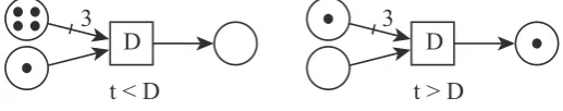
Figure 1 shows the features of a PN. The two nodes types, namely places and transitions, are shown as circles and squares respectively. The nodes are joined by directed edges seen as arrows. Although no two nodes of the same type may be directly connected, there is no limit on the number of inputs or outputs that can be associated with one node. If there are multiple directed edges between common nodes, they can be condensed into a single ‘weighted edge’ with the number of represented edges displayed numerically adjacent. If the weight of the edge is one, it is custom to omit the numerical label. Figure 1 includes a weighted edge, shown inputting to the transition. Places may contain solid dots known as tokens; a PN containing tokens is known as a marked PN. The location of tokens in a PN indicates the state of the system at that time. As tokens move through the PN the state of the system changes, it is the tokens therefore that allow the PN to model dynamic processes. The movement of tokens in a PN is facilitated by the firing of transitions. In order to fire a transition must first be enabled, this requires all of the input places to be populated with at least as many tokens as the weight of the respective directed edges inputting to the transition. In Figure 1 the transition is initially enabled. Once enabled a transition will fire immediately unless a delay is associated, in which case the transition will fire once the delay time, D, has passed. Upon firing, a transition will remove tokens from the input place(s) in a quantity that matches the weight of the respective input directed edge(s), destroy them, create new tokens and add them to the output place(s) in a quantity that matches the weight of the respective output directed edge(s). In Figure 1 once the delay time has passed, the transition removes three and one tokens from the input places and adds a single token to the output place.

3 3

D D

t < D t > D

Figure 1: Petri net firing process

Figure 2 contains a edge with a circle at its tip, as opposed to an arrowhead, this is known as an inhibit edge and is used to stop a transition from firing when otherwise enabled. As with directed edges, inhibit edges can be weighted, requiring a number of tokens to be present in the input place before a transition will be prevented from firing. Figure 2 shows the inhibit edge preventing the enabled transition from firing, even after the time delay has been satisfied.

D 2 D 2

t < D t > D

3 3

3

Fuel Rig System

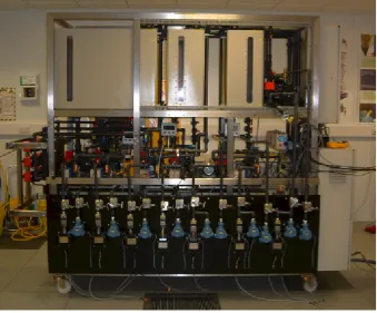
The proposed technique of system modelling and fault verification has been developed using the BAE Systems Advance Diagnostic Test Facility (ADTF). The ADTF, or fuel rig, consists of a set of tanks, pumps, valves and sensors which can be arranged to represent the fuel system. It is possible to inject a range of fault types into the fuel rig to mimic those that may occur during the phased mission of an aircraft. Figure 3 shows the fuel rig set-up.

Figure 3: BAE Systems Advanced Diagnostic Test Facility

3.1 System Description

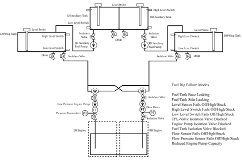
A schematic diagram of the fuel rig is shown in Figure 4. The fuel rig contains four fuel tanks, two auxiliary tanks which feed directly to one of the two wing tanks through an auxiliary fuel pump. Each tank has a level sensor, high level switch, low level switch and a drain valve. The wing tanks can feed to either engine pump, the flows being controlled by two triple port L-valves. In normal system operation the valves are set to theon

position and the flow paths are from the left hand (LH) wing tank to the LH engine pump and from the right hand (RH) wing tank to the RH engine pump. By setting a triple port L-valve tocrossfeedthe flow path can be set to feed an engine pump from a tank on the oppoise side of the rig, i.e. LH wing tank to RH engine pump. If inshutoff mode, the triple port L-valve prevents any flow reaching the engine pump. A singular sump tank represents the presence of engines on an aircraft fuel system on the fuel rig. Water is collected in the sump tank and used to refill the tanks through a series of pipes and pumps not shown on Figure 4.

Figure 4 lists a subset of faults that can be replicated on the fuel rig. It is possible to induce these faults either manually or remotely using the computerised interface that controls the fuel rig.

FT

PT FT FT PT

LH Auxiliary Tank Low Level Switch

Level Probe

RH Auxiliary Fuel Pump Drain

Level Probe LHWing Tank

Drain

RHWing Tank

Isolation Valve

Low Pressure Engine Pump

Pressure Transmitter

LH Engine

Isolation Valve

Flow Meter

Isolation Valve

RH Engine RH Auxiliary Tank

Low Level Switch High Level Switch

Drain Isolation Valve

LH Auxiliary Fuel Pump

High Level Switch

Level Probe

Low Level Switch High Level Switch Isolation

Valve IsolationValve

Fuel Rig Failure Modes

Fuel Tank Base Leaking Fuel Tank Side Leaking

Level Sensor Fails Off/High/Stuck High Level Switch Fails Off/High/Stuck Low Level Switch Fails Off/High/Stuck TPL-Valve Isolation Valve Blocked Engine Pump Isolation Valve Blocked Fuel Tank Isolation Valve Blocked Flow Sensor Fails Off/High/Stuck Flow Pressure Sensor Fails Off/High/Stuck Reduced Engine Pump Capacity

Figure 4: BAE Systems Advanced Diagnostic Test Facility schematic and possible failure modes

3.2 Operational Phases

Several potential operational phases of the fuel rig have been identified and are defined by setting the position of the triple port L-vales and the throttle demands of the pumps. In the first phase all the pumps and the triple port L-valves on the system are off. In this arrangement there is no flow in the system. In the second phase both triple port L-valves are set to on and the engine pumps activated. This creates two flow paths in the system, one from the LH wing tank to the LH engine and one from the RH wing tank to the RH engine. The third phase replicates the second but also activates the auxiliary pumps thereby creating two additional flow paths from the LH auxiliary tank to the LH wing tank and from the RH auxiliary tank to the RH wing tank. In the fourth phase the triple port L-valves are set such that the LH wing tank provides flow to both engines, there is no flow from the auxiliary tanks. Phase five replicates phase four but includes flow from the LH auxiliary tank to the LH wing tank. Phase six is similar to phase four except that the RH wing tank provides the flow to the engines and in phase seven the RH auxiliary tank feeds the RH engine tank to support it feeding both engines. The above does not represent an exhaustive list of operational phases, many more could be created using the distinction of engine throttle ratings as changing these will also change the system behaviour.

4

Fuel Rig Petri Net Model

The fuel rig described in Section 3 has been modelled using the PN technique. The system was modelled at component level including detail of the system’s different operational phases thereby allowing a phased mission to be represented.

automatically determined by the software from the fuel rig data log file and the appropriate number of tokens are added to the tank level places to replicate this. The PN model is capable of inducing any of the system faults listed in Figure 4.

The fuel tanks, which are 60cm tall on the physical fuel rig, have been modelled using place nodes such that a full fuel tank is represented by the place containing 50 tokens. Each token therefore represents 2% of the tank volume or an increase of 1.2 cm in the tank level. Further places are also included in the PN model to allow the tank levels to be represented with a greater level of detail.

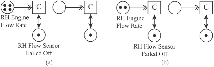
In addition to the standard PN features and ‘rules’, an additional transition type has been created to make modelling the fuel rig system more efficient. The ‘clear’ transition will remove all tokens from one of the input place nodes. Figure 5 illustrates how the clear tranisition works in two different scenarios. In both situations all of the tokens from the ‘RH Engine Flow Rate’ place have been removed. The double headed arrowhead displays graphically from which place the tokens will be removed upon firing.

C

C

C

C

RH Engine Flow Rate

RH Flow Sensor Failed Off

RH Engine Flow Rate

RH Flow Sensor Failed Off

(a) (b)

Figure 5: Clear transition removing tokens from flow rate place in (a) and (b)

The clear transition is effective when modelling the failure of a sensor, such as the ‘RH Flow Sensor Failed Off’ fault modelled in Figure 5. In the fuel rig PN model, the ‘RH Engine Flow Rate’ place may contain up to five tokens. With the clear transition modelling the failure of this sensor requires only one transition whereas without it at least five transitions would be required.

The fuel rig PN model contains 222 places and at least 433 transitions, the number of transitions will increase with the number of phase changes in a mission.

5

Standard Deviation Technique

A SD value offers a measure of the magnitude of variation present in the values of a data set compared to its mean value. The smaller this SD value, the closer all of the values in the data set are to the mean value.

The SD formula is presented in Equation 1. In the formulaxirepresents a data set value,¯xthe average of the

data set andnthe size of the data set.

SD=

v u u u t

n

P

i=1

(xi−¯x)2

(n−1) (1)

Each of the three variable types, tank level, flow rate and flow pressure rate, will have a maximum tolerance that the SD must be lower than in order for a fault to be verified. If any of the eight SD values exceed their tolerance, the fault will be considered false.

As this fault verification technique is concerned with faults generated during the start-up of complex systems all of the necessary data will be available from the system in order to apply the SD technique.

The fault verification process has also been automated in the PN software.

6

Results

This section presents and discusses the results of applying the SD technique to data outputs from the fuel rig system and PN model. Using known ‘no fault’ or nominal data from the fuel rig system, the PN system model was verified as correct and accurate. Fuel rig data recorded in the presence of faults was also considered to ensure failure modes were accurately represented in the PN model.

Data has been recorded for twenty-two different failure modes of the fuel rig system. In each case the fault was injected into the fuel rig during a phased mission. The mission consisted of five phases, extending over a period of 300 seconds. Using the phase numbering established in Section 3.2, in the first mission phase the fuel rig system was in operational phase one, no flow through the system. After fifteen seconds the fuel rig transitioned to mission and operational phase two, both engine pumps set to a demand of 50% creating flow paths from the LH and RH wing tanks to the LH and RH engines. After ninety seconds the fuel rig transitioned to mission and operational phase three as the auxiliary pump demand was set to 75% and flow paths were established from the LH and RH auxiliary tanks to the LH and RH wing tanks. After ninety seconds the fuel rig transitioned to mission phase four and reverted back to operational phase two, only flow paths from LH and RH wing tanks to LH and RH engines. After a further ninety seconds the fuel rig returned to operational phase one as it entered the final mission phase for a period of fifteen seconds. In each phased mission the fault was injected into the fuel rig after sixty seconds, during operational phase two.

6.1 Pump vibration effects

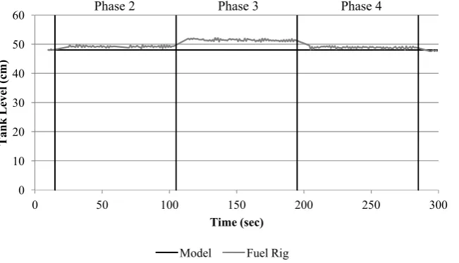
The engine pumps of an aircraft fuel system are represented on the fuel rig using peristaltic pumps. When operational the rotational motor within the pumps causes the fuel rig to vibrate. The effect is greater as the pump demand is increased and the motor turns at a greater speed. Figure 6 shows the effect of the vibrations on the RH auxiliary fuel tank level. The figure shows the tank levels recorded for the phased mission described above but with the auxiliary tank isolation valve closed to prevent any fluid leaving the tank.

It can be seen that at the start of phase three as the auxiliary pump demand is created there is a significant increase in the tank level. A similar effect can be seen at the start of phase two when the engine pump demand is established. Both of these increases are related to the pump induced rig vibrations that cause the fluid in the fuel tanks to shake. As would be expected once the pump demands are removed at the start of phases four and five the tank level falls. This coincides with the pumps turning off and no longer creating a vibration in the system. As the isolation valve from the auxiliary tank is closed all of these level changes occur with no fluid loss or gain in the tank.

The figure also shows that when there is a demand to the auxiliary pump the recorded tank level is noisier than when only the engine pump is active. Similar results can be seen with the wing tank level variables. Figure 7 shows the RH wing tank level over the course of the phased mission. As the RH auxiliary tank isolation valve is closed the wing tank does not receive any input flow in phase three.

0 10 20 30 40 50 60

0 50 100 150 200 250 300

T

an

k

L

eve

l(

cm

)

Time (sec)

Model Fuel Rig

Phase 2 Phase 3 Phase 4

Figure 6: RH auxiliary tank level

0 5 10 15 20 25 30 35 40 45

0 50 100 150 200 250 300

T

an

k

L

eve

l(

cm

)

Time (sec)

Model Fuel Rig

Phase 2 Phase 3 Phase 4

Figure 7: RH wing tank level

pump induced system vibrations are affecting both the auxiliary and wing tanks on the fuel rig. It is therefore necessary to attempt to quantify these vibrations effects to enable accurate fault verification.

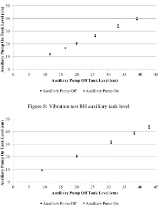
The auxiliary pump vibration effect will be quantified by comparing the recorded tank levels when only the engine pumps are on and when the engine and auxiliary pumps are on. During the tests the auxiliary and engine tank isolation valves were closed to prevent any flow leaving the tanks. The tests were performed at a number of tank level heights to investigate if the vibration effect varied with tank level.

Figure 8 and Figure 9 show the auxiliary engine off vs auxiliary engine on tank levels for the RH auxiliary and wing tank respectively. Both figures show a clear increase in the tank level when the auxiliary tanks are on and that the effect is greater at higher tank levels. Using the gradient of a linear trendline through the points plotted when the auxiliary engine is on, the vibration effect on each of the four tanks can be roughly quantified.

0 10 20 30 40 50

0 5 10 15 20 25 30 35 40 45

A u xi li ar y P u m p O n T an k L eve l( cm )

Auxiliary Pump Off Tank Level (cm)

Auxiliary Pump Off Auxiliary Pump On

Figure 8: Vibration test RH auxiliary tank level

0 10 20 30 40 50

0 5 10 15 20 25 30 35 40 45

A u xi li ar y P u m p O n T an k L eve l( cm )

Auxiliary Pump Off Tank Level (cm)

Auxiliary Pump Off Auxiliary Pump On

Figure 9: Vibration test RH wing tank level

L0= (L∗1.08) + 0.3 (2)

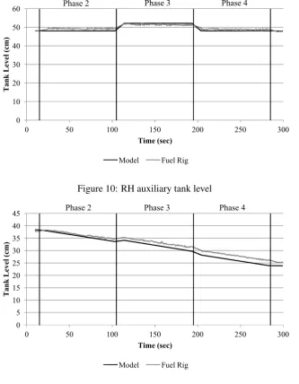
6.2 Verifying a genuine fault

The ability of the software to verify the failure mode ‘RH Auxiliary Tank Isolation Valve Blocked’ will be considered in more detail. The effect of this fault occuring, in the context of the phased mission described above, should be to prevent a flow path from the RH auxiliary tank to the RH wing tank in mission phase three. The consequences of the fault should be clear in the outputs of the RH auxiliary tank level and the RH wing tank level. Figure 10 and Figure 11 show the values recorded from the fuel rig and predicted by the PN model for these variables over the course of the phased mission. It should be noted that due to system noise present at the start of the mission and immediately after phase changes data from these parts of the mission are ignored so as not to bias the fault verification results.

0 10 20 30 40 50 60

0 50 100 150 200 250 300

T

an

k

L

eve

l(

cm

)

Time (sec)

Model Fuel Rig

Phase 2 Phase 3 Phase 4

Figure 10: RH auxiliary tank level

0 5 10 15 20 25 30 35 40 45

0 50 100 150 200 250 300

T

an

k

L

eve

l(

cm

)

Time (sec)

Model Fuel Rig

Phase 2 Phase 3 Phase 4

Figure 11: RH wing tank level

The SD of the RH wing tank level residuals is 0.58cm and for the LH wing tank residuals is 0.54cm. The SD of the auxiliary tank level residuals are 0.89 and 0.67cm for the RH and LH tanks respectively. Given the SD tolerance for the wings tanks is 1.5cm, it can be concluded that the PN model has accurately modelled the behaviour of the fuel tanks in the presence of a fault on the RH side and in normal operation on the LH side of the system. Had the impact of the pump vibrations not been taken into account the SD of the LH and RH auxiliary tank level residuals would have been 1.09 and 1.24cm. With these values even a small increase in the system noise or a short period of increased vibration beyond that accounted for could have caused the tolerance level to be exceeded and the fault report to be ignored. The SD of the LH and RH wing tank level residuals would have been 0.66 and 0.75cm had the pump vibrations not been accounted for. The technique applied to account for the pump vibrations can therefore be considered appropriate.

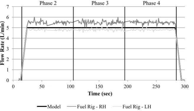
Figure 12 and Figure 13 show the LH and RH flow rate and the RH flow pressure variable over the course of the phased mission. Theoretically, in spite of the fault, the LH and RH engine pump demands should be satisfied throughout the mission, as neither wing tank level falls to zero. The figures show that the fuel rig behaviour matches that predicted and the PN model has represented this behaviour well.

0 1 2 3 4 5 6 7

0 50 100 150 200 250 300

Flow R

at

e (

L

/m

in

)

Time (sec)

Model Fuel Rig - RH Fuel Rig - LH

Phase 2 Phase 3 Phase 4

Figure 12: Fuel rig engine flow rates

0 5,000 10,000 15,000 20,000 25,000 30,000

0 50 100 150 200 250 300

F

low

P

re

ss

ur

e

(P

a)

Time (sec)

Model Fuel Rig

Phase 2 Phase 3 Phase 4

Figure 13: RH engine flow pressure

be as great as others. The pipe configuration to the LH and RH engine pumps from the wing tanks is also not consistent. The longer series of piping feeding the LH engine pump will exhibit a lower back pressure which will result in a reduced flow rate. The operation of the peristaltic pumps also creates distorted, irregular flow which affects the flow rate values recorded. Finally measurement variances at the flow meter could cause inac-curacies in the flow rates recorded. Nonetheless the SD results for the LH and RH flow rate values were 0.09 and 0.18L/min respectively. Given a proposed tolerance of 0.3L/min, the PN model results can be considered an accurate representation of the behaviour of the flow rate variable.

The SD results for the LH and RH engine flow pressure variables were 729 and 1,833Pa respectively. A tolerace of 8,500Pa is proposed for this variable and therefore both results would have passed their particular tests thereby contributing to the overall verification of the fault. A relatively high tolerance can be applied to the flow pressure variable due to the scale of the values recorded. Table 3 shows that when the predicted and actual flow pressure variable results are not similar the SD significantly exceeds the tolerance level proposed.

6.3 Verifying Leak Arisings

The only fault type that is not evaluated using the technique described above is a tank leak. It is necessary to consider leak fault reports separately because depending on the size and location of the leak the symptoms observed in the system will be different.

The process created to verify a leak fault report considers both the tank level and flow rate variables of the tank under consideration. In order to compare the two variables directly, the flow rate data must be converted into tank level values. Equation 3 is used to convert the flow rate data (F Ri) at every timestep (∆t) in the

mission into the volume of liquid that leaves/enters the tank (V). Both flow rates out of and into the tank under consideration must be subject to Equation 3. Equation 4 then converts the volume into a change in the tank level (L0) using the tank cross sectional area (CSA). Given the initial tank level this result can be used to give the flow rate determined tank level throughout the mission.

V = F Ri+F Ri+1

2 ∗∆t∗1000 (3)

L0= V

CSA (4)

In Equation 3 the flow rate data is measured inL/sec. The volume is expressed incm3. The cross sectional area of the tank is measured incm2_{and the change in tank level is expressed incm.}

To reduce the noise effects seen in the tank level graphs of Figures 6, 7, 10 and 11 a 10-point moving average has been applied to the level sensor data. This filter determines a tank level by averaging the nine previous data points with the point under consideration. This significantly reduces the noise in the level sensor output and enables a more accurate comparison with the flow rate data to be carried out.

Using the same phased mission described previously, a leak was injected into the side of the LH auxiliary tank of the fuel rig after 60 seconds. For this test a flow rate meter was placed at the outlet from the LH auxiliary tank thereby ensuring flow rates out of the auxiliary tank were measured. The structure of the system means there can be no flow into the auxiliary tanks and therefore only the flow rate out of the tank had to be monitored. Figure 14 shows the tank levels for the LH auxiliary tank over the course of the mission as determined from the moving averaged level sensor data and the flow rate data.

The figure shows that the initial effects of the leak in phase two are only visible from the level sensor data. This is a result of the fact that only the level sensor results include the effect of the leak. As none of the leak flow passes through the flow rate meter its effects are not captured in the flow rate data. The flow rate determined tank level only falls in phase three when the auxiliary pump is on. At the start of phase three the level sensor curve also becomes steeper indicating an increased flow out of the tank. This effect however only lasts until the middle of the phase when the gradient becomes more gradual. This change is a result of the tank level falling below the height of the leak and no longer having an effect. Beyond this point the gradients of the level sensor and flow rate tank level curves are similar.

To verify the presence of a leak fault report the tank level gradients prior to and after the fault report time are assessed. Gradients,m, are calculated from the data recorded by both the level sensor and flow rate data using Equation 5.

m= y2−y1

x2−x1 (5)

0 5 10 15 20 25 30 35 40 45

0 50 100 150 200 250 300

T

an

k L

eve

l (

cm

)

Time (sec)

Time Averaged Tank Level (Level Sensor) Tank Level (Flow Rate Sensor) Phase 2 Phase 3 Phase 4

Figure 14: RH wing tank levels

allow the moving averaged level sensor values to settle. The second data point is the time of the fault report. By treating the fault report time as a phase change, the data points used in Equation 5 to find the post fault report gradients are 20 and 30 seconds after the time of the fault report.

In order to verify the presence of a leak the gradient residual prior to and after the fault report must be consid-ered. The gradient residual is found by subtracting the flow rate tank level gradient from the level sensor tank level gradient. If a leak is present the gradient residual after the fault report will be less than prior to the fault report. A leak will be verified if the gradient residual after the fault report is lower than the gradient residual value prior to the fault less 0.019cm/sec. Equation 6 expresses this as an equation where RGrad−P re is the

gradient residual prior to the arising andRGrad−P ost is the gradient residual after the airisng.

RGrad−P ost< RGrad−P re−0.0190 (6)

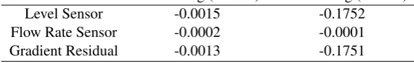
In the phased mission considered above the fault report occurs in the second phase of the mission which began after 15 seconds. The leak fault report was recorded at 60 seconds. The pre fault report tank level gradients are therefore found using the tank level and flow rate sensor data points at 35 and 60 seconds. The post fault report gradients are found using the data points at 80 and 90 seconds. Table 1 lists the tank level gradient values found using the above equations and the gradient residual values for the phased mission being considered.

Table 1: Level sensor and flow rate determined tank level gradients

Pre-Arising (cm/sec) Post-Arising (cm/sec)

Level Sensor -0.0015 -0.1752

Flow Rate Sensor -0.0002 -0.0001

Gradient Residual -0.0013 -0.1751

From Equation 6 and Table 1 it can be seen that if the gradient residual after the fault report was less than -0.0203cm/sec a leak would be verified. As this condition has been satisfied the presence of a leak in the LH auxiliary tank can be confirmed. The size of the leak is equivalent to the change of the gradient residual values - i.e. 0.1738cm/sec.

The final step, having verified the presence of a leak, is to identify the location or height of the leak. As was shown above, when a leak occurs the gradient residual value decreases. It follows then that if the tank level were to fall below the height of the leak the gradient residual value would increase to a value approaching that found prior to the leak appearing. It was shown previously that in order for a leak to be verified the gradient residual value after the fault report had to be at least 0.019cm/sec lower than the value prior to the report. It therefore follows that in order to confirm the tank level is below the leak height the residual gradient must be greater than the residual gradient prior to the arising less 0.019cm/sec.

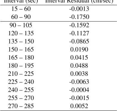
To find the leak height as accurately as possible gradient residual values are found at fifteen second intervals starting from the last time considered to find the post fault report gradients, i.e. thirty seconds after the fault report. The leak height will have therefore been identified if Equation 7 is satisfied. In the equationRGrad−P re

is the gradient residual prior to the arising andRGrad−Intervalis the gradient residual at the time of an interval.

RGrad−Interval> RGrad−P re−0.0190 (7)

Using the gradient residuals calculated above when the leak was verified, if the gradient residual at any interval is greater than -0.0203cm/sec then the tank level will have dropped below the leak height.

Table 2 lists the gradient residuals for the phased mission described above. Intervals which include data that falls within the first ten seconds of a phase are ignored due to phase transition effects.

Table 2: Residual Values After Arising

Interval (sec) Interval Residual (cm/sec)

15 – 60 -0.0013

60 – 90 -0.1750

90 – 105 -0.1592

120 – 135 -0.1127

135 – 150 -0.0865

150 – 165 0.0190

165 – 180 0.0415

180 – 195 0.0488

210 – 225 0.0038

225 – 240 -0.0063

240 – 255 -0.0004

255 – 270 -0.0015

270 – 285 0.0052

6.4 Assessing genuine and false faults

In addition to verifying the presence of genuine faults, the proposed fault verification technique must also filter false faults. By evaluating a health log file that contains multiple fault reports, where only one is true, the ability of the software to both verify genuine and filter false faults will be established.

Using the five phase mission described previously, the fault ‘RH Flow Pressure Sensor Failed Off’ has been induced in the fuel rig. The additional false faults included in the health log file are ‘RH Flow Pressure Sensor Failed Stuck’, ‘RH WT Isolation Valve Blocked’ and ‘RH Flow Sensor Failed Stuck’. Including two failure modes of the same component will ensure the PN and fault verification software can decipher between them.

Table 3 lists the SD results of modelling the faults listed above and comparing the predicted system behaviour with that of the fuel rig when the ‘RH Flow Pressure Sensor Failed Off’ fault was injected. Those SD results that exceed the variable tolerance are highlighted in bold.

Table 3: Failure Mode SD Results

Failure Mode Pressure Sensor Pressure Sensor Wing Tank Iso- Flow Sensor

Failed Off Stuck Valve Blocked Stuck

RH Wing Tank 0.46 0.46 4.30 0.46

LH Wing Tank 0.56 0.56 0.56 0.56

RH Auxiliary Tank 0.93 0.93 0.93 0.93

LH Auxiliary Tank 0.49 0.49 0.49 0.49

RH Flow Rate 0.19 0.19 1.99 0.77

LH Flow Rate 0.11 0.11 0.11 0.11

RH Flow Pressure 751 46,830 38,260 46,736

LH Flow Pressure 1,467 1,467 1,467 1,467

As only faults on the RH side of the fuel rig system have been considered, the SD results of the variables on the LH side are the same irrespective of the failure mode. Considering the false faults modelled by the software, Table 3 shows that the RH flow pressure tolerance level has been exceeded in all three scenarios. In the case of the wing tank isolation valve blocked and flow sensor stuck faults, additional results have exceeded the tolerance levels of the respective variables.

Figure 15 shows the predicted flow pressure behaviour when all of the faults considered are propagated through the PN model. Also plotted is the flow pressure recorded from the fuel rig during the mission. When the flow pressure sensor fails off it outputs a value of -103,500Pa. This value represents the zero volt value of the flow pressure sensor after having been converted from a voltage to a pressure value.

Figure 15 shows that the predicted and actual flow pressure behaviour is only similar when the flow pressure sensor fails off fault is modelled. In the other scenarios the predicted behaviour is significantly different from that recorded on the fuel rig. Due to this and the scale of the flow pressure variable, the SD results of the false faults exceed the tolerance of 8,500Pa by a large margin.

Using the SD results of the RH flow pressure variable alone it can be seen that the fault verification process has successfully identified the false faults which would enable them to be filtered. Tolerance levels have also been exceed in the RH flow rate and RH wing tank variable results. Given the failure modes propagated through the PN model in these instances, these results could have been predicted and are therefore correct.

-120,000 -100,000 -80,000 -60,000 -40,000 -20,000 0 20,000 40,000

0 50 100 150 200 250 300

F

lo

w

P

re

ss

ur

e

(P

a)

Time (sec)

Fuel Rig Data Pressure Sensor Failed Off Wing Tank Iso Valve Blocked Flow Sensor Stuck Pressure Sensor Stuck

Phase 2 Phase 3 Phase 4

Figure 15: RH engine flow pressure rate

7

Conclusions

This paper has shown how a PN system model can be combined with the SD technique to assess and verify fault reports generated by the health management systems of complex phased mission systems. The proposed technique has been tested using a phased mission devised for a mechanical rig representing an aircraft fuel system.

The proposed technique uses PNs to create a model of the system under consideration. By injecting the fault reports generated by the health management system into the PN model, their effect can be propagated and the behaviour of the system variables predicted. Residual values of the system variables can then be calculated by subtracting the PN predicted values from those recorded from the system. Using these residuals SD values are calculated that indicate the similarity of the PN predicted system behaviour to that recorded. If the SD values of all the variables fall within the pre-set tolerances, the fault under consideration is verified as genuine. However, if any SD values exceed the tolerances the fault is considered false and can be ignored/filtered. The results of applying this technique to the fuel rig system have shown it to be successful in both verifying genuine faults and filtering false faults. This also demonstrates that the PN model has accurately represented the behaviour of the system.

A technique has also been developed to deal with leak arisings in a detailed and accurate manner. By evaluating the level sensor and flow rate data the presence of a leak is first assessed. If the presence of a leak is verified the height of the leak in the tank is then considered. The approach has been shown to be both versatile enough to work in multi-phased mission systems and capable of determining leak heights with a high level of accuracy.

Vibration issues were created in the fuel tanks of the fuel rig by the peristaltic pumps. The issue was accounted for using tank specific correction factors. The variables recorded from the fuel rig system have also been shown to be quite noisy. The fuel rig system has therefore shown that the proposed techniques are capable of verifying the legitimacy of faults in challenging situations. In less noisy systems the same techniques could be applied with narrower tolerances to filter a greater number of false faults.

Acknowledgements

*The Lloyd’s Register Educational Trust (The LRET) is an independent charity working to achieve advances in transportation, science, engineering and technology education, training and research worldwide for the benefit of all.

References

[1] E. Gascard, Z. Simeu-Abazi, and Y. Joseph. Exploitation of built in test for diagnosis by using dynamic fault trees: Implementation in matlab simulink. InAdvances in Safety, Reliability and Risk Management: ESREL 2011, pages 436–444. CRC Press, August 2011. OSP.

[2] K. Westervelt. Root cause analysis of bit false alarms. InAerospace Conference, 2004. Proceedings. 2004 IEEE, volume 6, pages 3782 – 3790 Vol.6, March 2004.

[3] S. L. Salem, G. E. Apostolakis, and D. Okrent. A new methodology for the computer-aided construction of fault trees. Annals of Nuclear Energy, 4:417–433, 1977.

[4] A. Carpignano and A. Poucet. Computer assisted fault tree construction: a review of methods and con-cerns.Reliability Engineering & System Safety, 44:265–278, 1994. Special Issue On Advanced Computer Applications.

[5] S. A. Lapp and G. J. Powers. Computer-aided synthesis of fault-trees. IEEE Transactions on Reliability, R-26:2–3, April 1977.

[6] P. K. Andow. Difficulties in fault-tree synthesis for process plant. Reliability, IEEE Transactions on, R-29:2–9, April 1980.

[7] C. Petri. Kommunikation mit Automaten. PhD thesis, Institut fur instrumentelle Mathematik, Bonn, 1962.

[8] S.P. Chew, S.J. Dunnett, and J.D. Andrews. Phased mission modelling of systems with maintenance-free operating periods using simulated petri nets.Reliability Engineering & System Safety, 93:980–994, 2008.

[9] Michael D. Lloyd. Phased mission approach to fault propagation. Technical report, University of Not-tingham, 2011.

[10] Jospeh B. Kruskal and Mark Liberman. The symmetric time-warping problem: from continuous to dis-crete. Addison-Wesley, 1983.

[11] Fausto P. Garc´ıa, Diego J. Pedregal, and Clive Roberts. Time series methods applied to failure prediction and detection. Reliability Engineering & System Safety, 95:698–703, 2010.

[12] Tadeo Murata. Petri nets: Properties, analysis and applications.Proceedings of the IEEE, 77(4):541–580, April 1989.

[13] James L. Peterson. Petri nets.ACM Computing Surveys, 9:223–252, 1977.

[14] K. Jensen. Coloured Petri Nets: Basic Concepts, Analysis Methods and Practical Use. Monographs in Theoretical Computer Science. Springer-Verlag, 1997.