Exact Solutions for a Class of Nonlinear PDE with Variable Coefficients Using ET and ETEM

(1)

https://www.scirp.org/journal/jamp ISSN Online: 2327-4379

ISSN Print: 2327-4352

DOI: 10.4236/jamp.2019.711183 Nov. 5, 2019 2685 Journal of Applied Mathematics and Physics

Exact Solutions for a Class of Nonlinear PDE

with Variable Coefficients Using ET and ETEM

Shifei Sun, Lina Chang, Hanze Liu

School of Mathematical Sciences, Liaocheng University, Liaocheng, China

Abstract

In this article, by using the modified CK direct method, we give a relationship between the generalized fifth-order KDV equations with variable coefficients and the corresponding constant coefficients ones. Then, we construct the ab-undant travelling solutions by the extended trial equation method (ETEM) in terms of different functions, such as the elliptic functions, rational functions, hyperbolic functions and trigonometric functions. The extended trial tion method is powerful and can be used to other partial differential equa-tions and more research can be done by this method.

Keywords

Equivalence Transformation, Extend trial Equation Method, Higher Order Partial Differential Equation, Travelling Wave Solution

1. Introduction

It is well known that the exact solutions of partial differential equations are an important problem in nonlinear science; the travelling wave solutions of partial differential equations with variable coefficients are always playing an important role in studying the long-time behavior of solutions and understanding the com-plex nonlinear fluctuations. Especially in the multifarious real physical back-ground such as the field of nonlinear optical crystal and plasma, nonlinear par-tial differenpar-tial equations (PDEs) with variable coefficients can often provide rea-listic and powerful models than the corresponding constant coefficients ones when the inhomogeneities of media are considered. There are lots of studies have been conducted with different types of the PDEs, such as the modified trigono-metric functions series [1] [2], the G G′ expand method [3] [4], the first integral

method [5] [6], the modified CK direct method [7] [8] [9], the exp

(

−φ ξ

( )

)

method [10] [11], modified simple equation method [12] [13], infinite series How to cite this paper: Sun, S.F., Chang,

L.N. and Liu, H.Z. (2019) Exact Solutions for a Class of Nonlinear PDE with Variable Coefficients Using ET and ETEM. Journal of Applied Mathematics and Physics, 7, 2685- 2700.

https://doi.org/10.4236/jamp.2019.711183

Received: October 16, 2019 Accepted: November 2, 2019 Published: November 5, 2019

(2)

DOI: 10.4236/jamp.2019.711183 2686 Journal of Applied Mathematics and Physics

method [14] [15], the Lie symmetry analysis method [16]-[21] and the extended trial equation method [22] [23]. In this paper, we will use the modified CK direct method and the extended trial equation method (ETEM) to discuss the exact solutions for the following generalized fifth-order nonlinear partial differential KDV equation [24] [25] [26] [27] with time-dependent variable coefficients of the dispersion:

( )

2

( )

2

( )

3

( )

5

2 3 5.

u u u u

t u u t F t u G t

x x x x x

u

t α β

∂ ∂ ∂ ∂ ∂

− − − −

∂ ∂ ∂

∂

∂ ∂

=

∂ (1)

here the derivative ut represents the time evolution of a travelling wave as it travels in a certain direction, the function of nonlinear terms 2

,

x x xx u u u u and xxx

uu are to collect the waves and the function of the linear term

u

_xxxxx is to

disperse the waves, respectively,

α

( ) ( ) ( ) ( )

t ,

β

t ,F t G t, are arbitrary smooth

functions of t. When

α

( ) ( ) ( ) ( )

t ,

β

t ,F t G t, be constant, the Equation (1) be

the generalized fifth-order KDV equation. What’s more, we can get many other famous fifth-order partial differential equations by taking different values of the parameters:

Sawada-Kotera (SK) equation: when 5, 2, 1 2 F

F G

β = = α = =

2

5 5 5 0.

t x x xx xxx xxxxx u + u u + u u + uu +u =

Caudrey-Dodd-Gibbon (CDG) equation: when 30, 2, 1 5

F

F G

β = = α = =

2

180 30 30 0.

t x x xx xxx xxxxx

u + u u + u u + uu +u =

Lax equation: when 3 2

2 , , 1

10

F F G

β = α = =

2

30 20 10 0.

Kaup-Kuperschmidt (KK) equation: when 10, 5 , 2, 1

2 2

F

F= β = F α = G=

2

50 25 10 0.

Ito equation: when 3, 2 , 2 2, 1 9

F

F= β= F α = G=

2

2 6 3 0.

(3)

Lou modified the CK direct method and proposed a simple method which called the modified CK direct method. Furthermore, many scholars have studied the nonlinear equations with this method. In this paper, a new ETEM method is ap-plied to the variable coefficient KDV equation which is reduced by CK method for the first time, and a series of new exact solutions are obtained.

The aim of this research is to establish an equivalence relation between the va-riable coefficients PDE and the corresponding constant coefficients one, and use a variety of distinct trail equations to construct some new travelling wave solu-tions of the constant coefficients equation. In this way, we can obtain a series of new exact solutions of the variable-coefficient equation by the relation between the variable-coefficient equation and the constant-coefficient equation, such as the trigonometric function solution, soliton solution, periodic solution and ra-tional solution. In section 2, the equivalence relation between the fifth-order KDV equation with variable coefficient and the corresponding constant coefficient equation is given by using the modified CK direct method. In section 3, the ETEM is briefly introduced. In section 4, we obtain some new types of travelling wave solutions to Equation (1). In section 5, the more possibility of ETEM me-thod for solving partial differential equations is discussed. In section 6, the con-clusion and discussion are given.

2. Equivalence Transformations (ETs) of Generalized

Fifth-Order KDV Equation

In this section, we will use the modified CK direct method to look for the equi-valence transformations between Equation (1) and the corresponding following equation.

2

0,

u +au u +bu u +cuu +du = (2)

where a b c d, , , are arbitrary constants. Suppose that Equation (1) has the

fol-lowing solution:

( )

,

(

,

)

,

u x t = +A BU X T (3)

where A=A x t

( )

, ,B=B x t

( )

, ,X = X x t T

( )

, , =T x t

( )

, are functions can be

de-termined by requiring U =U X T

(

,

)

satisfy the transformation

{

x t u, ,

} {

→ X T U, ,

}

. in other words, we let

{

X T U, ,

}

to satisfied the

corres-ponding constant coefficients equation of Equation (1) as following

2

0.

T X X XX XXX XXXXX

U +aU U +bU U +cUU +dU = (4)

Then substituting Equation (3) into Equation (1), requiring U =U X T

(

,

)

and

T

U satisfied Equation (4), we can collect the coefficients of U, letting their

de-rivatives to be zero, we have

0,

xxxxx t GBX −dBT =

2 3

0,

x t

FB X −cBT =



3 2 2

15 10 0,

x x xx x xxx

(4)

DOI: 10.4236/jamp.2019.711183 2688 Journal of Applied Mathematics and Physics 10GBX Xxx xxx+5GBX Xx xxxx+3FBX X ax xx =0,

0,

xx x xxx xxxxx t

BX A FBX A GBX BX

β + + + =

2

0.

xxxxx x xx x xxx t GA +A

α

A +

β

A A +FA A+A =

Solving above equations, we have

0 3 5 2 3

2 0 2

0, , cTt , Tt , ,

A B C F G d X C x C

C C C

= = = = = +

2 3

2 0 2 0

, ,

t t

T T

a b

C C C C

α= β = ₍₆₎

where Tt is an arbitrary function of t, C C C1, 2, 3 are arbitrary constants. Then

with Equation (6), we can obtain new travelling wave exact solutions for the Eq-uation (1) as follows:

( )

(

)

0 2 3, .

u=C U C x+C T t (7)

If U X T

(

,

)

is the solution of fifth-order KDV equation with constant

coeffi-cients, then u x t

( )

, also is a solution of Equation (1).

3. Description of the Extend Trial Equation Method

In this section, we introduce the extend trial equation method (ETEM) as fol-lows.

Step1. Firstly, we consider the following nonlinear partial differential equa-tion:

(

)

1 , ,t x, xx, xt, tt, xxx, 0,

F u u u u u u u  = (8)

In order to look for the solutions of Equation (1), we make the travelling wave transformation

( )

,

( )

, u x t =U

ξ

where ξ = −x ct, and c is an arbitrary constant.

Then the Equation (8) can be converted to an ordinary differential equation as following

(

)

2 , , , , 0.

F U U U_ξ _ξξ U_ξξξ  = (9)

Step 2. We suppose that the exact solution of Equation (9) is of the form

1 , i i i

u Y

δ

τ =

=

∑

₍₁₀₎

where

τ

i

(

i=1, 2, 3,,

δ

)

are arbitrary constant, and i

Y satisfied the following

condition

( )

2

( )

_{( )}

0 1 2 2 2

0 1 2

,

Y Y Y Y

Y Y

Y Y Y Y

θ θ

ε ε

φ ξ ξ ξ ξ

ψ ζ ζ ζ ζ

+ + + + ′ = Λ = =

+ + + +



 (11)

where ξθ and ζε are arbitrary positive integers to be determined later.

Step 3. According to the balance principle we can determine a relation of θ,

(5)

(10) can be written as a series of infinity solutions.

Step 4. Substituting Equation (10) and Equation (11) into Equation (9), let-ting the coefficients of Y to be zero, by solving the system of algebraic equations by some software like Maple and Mathematica, we can figure out the values of

,

θ ε

ξ ζ and τδ, then reducing Equation (11) to the elementary form as follows:

(

)

( )

0

1

dY Y d ,Y

Y Y

ψ ξ η

φ

± − = =

Λ

∫

(12)

where η0 is an arbitrary constant.

Using a complete discrimination system for polynomial to classify the differ-ent forms of Equation (12), we can write the travelling wave solutions respec-tively. In this paper, the solutions of PDEs with variable coefficients also can be written respectively by the conclusion we got in the last section. Moreover, this method is appropriate for lots of other PDEs which can be discussed as follows.

4. ETEM to Generalized Fifth-Order KDV Equation

In this section, we discuss the generalized fifth-order KDV equation by using ex-tend trial equation method.

2

0.

u +au u +bu u +cuu +du = (13)

Using the travelling wave transformation

( )

,

( )

u x t =U

ξ

, where ξ = −x Ct,

Equation (13) turns into the following ordinary differential equation, then in-tegrate the equation once:

( )

2 ( )4

3

1 0,

3 2

a b c

C −CU+ U + − U′ +cUU′′+dU = (14)

where C1 is the integration constant. Substituting Equations (10) and (11) into

Equation (14)

1

1 0,

U =

τ

δYδ +

τ

δ−Yδ− + +

τ

3 3 3 3 3 3 3

1 0,

U =

τ

_δY δ +

τ

_δ−Y δ− + +

τ

(15)

(

)

2 2

1 2

1 , , , ,

U Y Y X Y

δ θ ε δ

δ

δτ − τ θ δ ε + − −

′= ′+= +

( )4

₍

₎

2 2 4

2 , , , .

U =X τ θ δ ε Yδ+θ−ε− + (16)

Using the balance principle, we find the highest degree terms of two Equa-tions (15) and (16) should be the same, so we have

2.

δ θ ε= − −

By assuming and assigning the variables that satisfy the above conditions, we can obtain the traveling wave solution of the Equation (13) in many cases.

If

ε

=0,

θ

=3 and δ =1, then

0 1 ,

U =τ +τY

2 3

0 1 2 3

1

0

,

Y Y Y

U τ ξ ξ ξ ξ

ζ

+ + +

(6)

(

2

)

1 2 3

1 0 2 3 , 2 Y Y

U τ ξ ξ ξ

ζ

+ +

′′ =

(

)

2 3

0 1 2 3 2 3

1 3

2 0

3 ,

Y Y Y Y

U τ ξ ξ ξ ξ ξ ξ

ζ

+ + + + ′′′ =

( )4 32 3 2 3 2 1 3 22 0 3 1 2

1 2

0

15 15 9 2 6

, 2

Y Y Y Y

U τ ξ ξ ξ ξ ξ ξ ξ ξ ξ ξ

ζ

+ + + + +

= ₍₁₇₎

where ζ ξ ≠0 3 0.

Substituting Equation (17) into Equation (14), collecting the coefficients of Y

and solving these algebraic equation systems respectively, we can obtain:

3 L1 0 1,

ξ = ζ τ

(

)

0 0 1

2

3 2

, L c a L

ζ τ

ξ = − +

(

)

(

)

2 2 2 2 2 2 2 2 2 2 2 2

0 1 0 1 2 0 1 0 2 0 2 0 0 2

1 2

1 2 1

9 3 12 2 4

, 9

L dc L L c L adc L a L ac da CL

L dL b

ζ τ τ τ τ τ τ

ξ τ − + − − + − + = + 0

ξ _{(See Appendixes A1), (18)}

where 1 2 2

2 40 4 4

30

c b ad b bc c

L

d

− − + − + + +

= ± _,

2 2 2

3 54 1 15 1 9 1

L = L d + L db− L dc b+ −bc, L2=15dL1+ +c b. We can use Equation

(18) and Equation (12) to get

(

)

( )

3 2

3 2 1 0

0

1

dY Y Y Y Yd .Y

Y

ξ ξ ξ ξ

ξ η

ζ

+ + +

± − = =

Λ

∫

(19)

Then, we will discuss some of the special form of solutions of Equation (14) as follow.

If Equation (19) can be written as following form:

(

)

(

)

(

)

(

3 2

3 2 1 0

0 1

3 2

1 1

2

2 2 2 2 2 2 2 2 2 2 2 2

1 0 1 2 0 1 0 2 0 2 0 0 2

2

1 2 1

3 2 2 3 3 3 3 3 3 2 3 3

0 0 2 2 0 2 0 1 1 2 0 2 1 0 2

3 2

9 3 12 2 4

9

2 6 3 27 9 3

Y Y Y Y

L c a

L Y Y

L

L dc L L c L adc L a L ac da CL

Y

L dL b

d L a L ab CL b C L L d c L L ac L

ξ ξ ξ ξ

τ τ

τ τ τ τ τ τ

τ

ζ τ τ τ τ τ

+ + + + = − − + − − + − + + + + − − + − − +

) (

)

(

)

2 3 2 3 2 3 3 3 2 3 3 3 2

0 2 0 2 0 1 0 1 2 0 2

3 3 3 3 3 2 3 2 2 3 2 2

1 2 0 1 2 0 0 2 1 0 2 0 1

2 3 2 2 3 3 2 2 3 2

0 1 0 1 2 0 1 2 0 1 2 2 1 3

3 1

6 3 81 24 3 6

9 27 54 24 162

108 72 9 9 3

.

ac L c L C d L c d a C L b d CL a

L L da CL L d c L L d c L da d L c a

d L ca c L L ad d L L ac d CL L c L L

Y

τ τ τ τ τ

α − − − − − + − + + + − − + − + = − (20)

where α1 is an arbitrary constant. Collecting the coefficients of Y of Equation

(7)

DOI: 10.4236/jamp.2019.711183 2691 Journal of Applied Mathematics and Physics 1 2 1 0 1 1 3 1 , , 3 3 L

L cL a

α

τ = τ =

+

(

)

(

)

2 3 2 2 2 2 2 2 2

1 1 1 2 1 1 1 2 1 2

2 2

1 1 1 1

3 135 18 180 9 6 12

60 12 4 2 3 2 ,

C L dc L L c L adc L bc aL L acL L

L da L abc a b L L c a

α

= − + + + −

+ + + +

`1

C (See Appendixes A2) (21)

In this family, Equations (18), (19) and (21) lead to get

2 3

3 0, 2 3 1 0, 1 3 1 0, 0 1 0.

ξ

=

ζ ξ

= −

α ζ ξ

=

α ζ ξ

= −

α ζ

₍₂₂₎

And

(

)

( )

₍

₎

0 3 1 2 1

1 d 2

dY Y .

Y Y _Y ξ η α α ± − = = = − − Λ ₋

∫

(23)

By Equation (23), (21), we can get the rational exact solution of Equation (14) as following

( )

(

)

1 2

1 1 ₀

3 1 4

.

3 3

L U

cL a L

α ξ α ξ η     = + + + __ ₋ __

( )

(

)

1 2 1 2

1 1 ₀

3 1 4

, ,

3 3

L u x t

cL a L _{x Ct}

α _α

η

 

 

= + +

+ _ − − _ (24)

where

(

)

(

)

2 3 2 2 2 2 2 2 2

1 1 1 2 1 1 1 2 1 2

2 2

1 1 1 1

3 135 18 180 9 6 12

60 12 4 2 3 2 ,

C L dc L L c L adc L bc aL L acL L

L da L abc a b L L c a

α

= − + + + −

+ + + +

Hence, with the relation of Equation (7) obtained above, Equation (1) have the following form of rational travelling wave solution

( )

(

)

2 2 1 0 2 2

0 ₂ ₂ 1 2

0

2 40 4 4

3 15

30 ,

2 40 4 4

3 3

30

1 4

,

2 40 4 4

30

c b ad b bc c

d c b

d

u x t C

c b ad b bc c

c a

d

C

X CT

c b ad b bc c

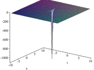
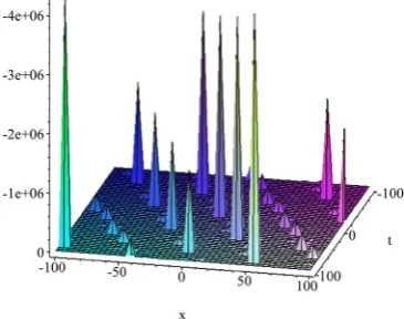
d α α η   _{− − + −} ₊ ₊ ₊    ± + +     _ _    =  _{− − + −} ₊ ₊ ₊  ± +         + +    − − + − + + + _ − − _ ±      (25)

where X =C x2 +C3, T is an arbitrary function of t (Figure 1 and Figure 2).

1) In the following, we chose some new coefficients to make it easier to calcu-late

3 L1 0 1, 2 L4 0 0,

ξ = ζ τ ξ = ζ τ

(

)

(

2 2 2 2

)

(

)

1 2 L d4 0 L c4 0 a 0 C 0 1 9dL4 b ,

ξ = − τ + τ − τ + ζ τ +

(

) (

)

3 3 2 3

0 0 1 0 0 1 0 0 1 1 1 4 0

2 3 3 2 3 3 3 2

4 0 0 0 4 0 4 0 4 0 1 3

2 9 27 3 27 3 6

3 3 3 3 3 3 3 .

adL ab dCL bC dL C bC cdL

c L ac cC d L adL dCL L

ξ ζ τ τ τ τ τ

τ τ τ τ τ τ τ

= − − + + − − +

(8)

[image:8.595.277.471.76.219.2]

Figure 1. The three-dimensional picture of the exact solution (25) of Equation

(1), and its projection at b=3,c=2,a= =d 1,η0=3 and α=11.

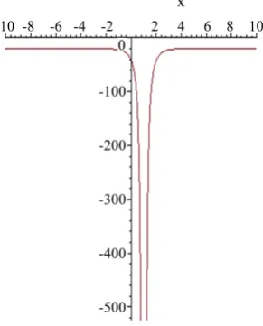
Figure 2. The two-dimensional picture of the equation

exact solution (25) of Equation (1), and its projection at 0

t= . When b=3,c=2,a= =d 1,η0=3 and α=11. where

2 2

1

2 40 4 4

, 30

c b ad b bc c

L

d

− − + − + + +

= ±

2 2 2

3 54 1 15 1 9 1 ,

L = L d + L db− L dc b+ −bc

(

) (

)

4 3 1 2 15 1 .

L = cL + a dL + +b c

If Equation (19) can be written as following form:

(

)

(

)

(

)

(

) (

)

2 2 2 2

4 0 4 0 0 0

3 2 3

1 1 4 0 2 1 0

1 4 1 5

3 2 3 2 3 3

0 1 0 0 1 1 1 4 0 4 0 0

2

2 3 3 3

0 4 0 4 0 4 0 2 3

2 ₁

9

9 3

27 3 27 3 6 3 3

3 3 3 3 ,

L d L c a C

L Y L Y Y adL

dL b L

ab dCL bC dL C bC cdL c L ac

cC d L adL dCL Y Y

τ τ τ ζ

τ τ τ

τ τ

τ τ τ τ τ τ

τ τ τ τ α α

− + − +

+ + + −

+

− + + − − + − +

− − − + = − −

(27)

where α α2, 3 are arbitrary constants. Collecting and letting all coefficients of Y

[image:8.595.293.453.265.454.2]

(9)

DOI: 10.4236/jamp.2019.711183 2693 Journal of Applied Mathematics and Physics 2 3 1 0 1 4 2 1 , , L L α α

τ = τ = +

(

)

2 2 2 2 2 2

1 4 2 1 4 2 3 1 4 3 1 4 1 1 4 2 3 2

4 1

2 2 2 2 2 2

1 4 4 4 1 4 2 3 1 2 1 2 3 1 3 1

17 26 2 8 8

2

2 2 8 8 2 ,

C L L d L L d dL L L L c L L c

L L

L L c L b L b L a L a L a

α α α α α α α

α α α α α α α α

= + + − −

− + + + + +

1

C (See Appendixes A3) (28)

In this family, Equation (18), (19) and (28) lead to get as follows:

(

)

(

)

2

3 0, 2 2 2 3 0, 1 2 2 2 3 0, 0 3 2 0,

ξ =ζ ξ = − α +α ζ ξ =α α + α ζ ξ = −α α ζ (29)

where ζ0 is an arbitrary constant.

When α α3− 2 >0,

(

)

(

)(

)

3 1

0 1

3 2 3 2

2

2 3

d 2

tan Y ,

Y

Y Y

α ξ η

α α α α

α α

−  − 

± − = = −  

− _ − _

− −

∫

(30)

we can solve for Y

(

)

2 3 2

(

)

3 3 2 tan 0 .

2

Y =α + α α−  α α− ξ η− 

 

  (31)

By Equation (31), (29), we can get the rational exact solution of Equation (14) as following

( )

2 3

(

)

2 3 2

(

)

3 3 2 0

4 1 2 1 tan . 2 U L L α α α α

ξ = + + α + α α−  − ξ η− 

 _ _

  (32)

With the relation of Equation (7), Equation (1) have the following form of ra-tional travelling wave solution

( )

(

)

(

)

(

)

2 2 2 3 0 2 2 2 2 3 2 2

3 3 2 0

2 40 4 4

2 15

30 ,

2 40 4 4

3 2

30

1

2 40 4 4

30

tan ,

2

c b ad b bc c

d b c

d u x t C

c b ad b bc c

c a

d

c b ad b bc c

d

X CT

α α

α α α η

   _{− − + −} ₊ ₊ ₊    +  _± _+ +     _ _ _ _  =    _{− − + −} ₊ ₊ ₊ ± +  _ _  _ _  +  _{− − + −} ₊ ₊ ₊  ±           −     × + −  − −    _ _  _{ }   (33)

where X =C x2 +C3, T is an arbitrary function of t. (Figure 3 and Figure 4)

When α α3− 2 <0,

(

)

2 3 2

(

)

2 2 3 csch 0 .

2

Y=α + α −α  α α− ξ η− 

 

  (34)

(10)

[image:10.595.282.465.75.219.2]

Figure 3. The three-dimensional picture of the exact solution (33) of

[image:10.595.212.537.504.700.2]

Equa-tion (1), Whenb=3,c=2,η0=1,a= =d 1 and α2=1,α3=5.

Figure 4. The two-dimensional picture of the equation exact solution (33) of Equation (1),

and its projection at t=0. When b=3,c=2,η0=1,a= =d 1 and α2=1,α3=5.

( )

(

)

(

)

(

)

2 2

2 3

0

2 2

2 3

2

2 2 3 0

2 40 4 4

2 15

30 ,

2 40 4 4

3 2

30

1

2 40 4 4

30

csch ,

2

c b ad b bc c

d b c

d u x t C

c b ad b bc c

c a

d

c b ad b bc c

d

X CT

α α

α α α η

   _{− − + −} ₊ ₊ ₊  

 +  _± _+ + 

 

 _ _ _ _

 =

 

 _{− − + −} ₊ ₊ ₊

± +

 _ _

 _ _



+

 _{− − + −} ₊ ₊ ₊ 

± 

 

 

  

  − _

 

× + −  − − 



 _ _

 _{ }

 

(35)

(11)

[image:11.595.272.476.74.229.2]

Figure 5. The three-dimensional picture of the exact solution (35) of

Equation (1), whenb=3,c=2,a= =d 1,η0=1 and α2=3,α3=1.

Figure 6. The two-dimensional picture of the equation exact

solution (35) of Equation (1), and its projection at t=0, when

0

3, 2, 1, 1

b= c= a= =d η = and α₂=3,α₃=1.

5. More Discussion

In this article, we obtained a series of exact travelling wave solutions of fifth-order KDV equation by the extended trail equation method; according to picking dif-ferent parameters we can get more exact analytic solutions of nonlinear partial differential equations like fifth-order KDV equation.

The extend trial equation method (ETEM) is proving to play an important role in solving partial differential equations, by using a variety of trail equations, we can construct lots of new types of travelling wave solutions. In this paper, we only considered the following parameters

0, 3, 1.

ε= θ = δ =

In a later study we can also study different situations such as δ ≠1 or ε ≠0.

[image:11.595.302.448.278.459.2]

(12)

(16). So we can take any other parameters that satisfies the following equation

2.

δ θ ε= − −

For example

1) When

ε

=0,

θ

=4 and δ =2.

( )

2

( )

_{( )}

₀ ₁ ₂ 2 ₃ 3 ₄ 4 0

,

Y Y Y Y Y

Y

ξ ξ ξ ξ ξ

ζ

Φ + + + + ′ = =

Ψ (36)

and

2

0 1 2 ,

U =

τ τ

+ Y+

τ

Y

(

)

2 3 4

1 2 0 1 2 3 4

0

2

,

Y Y Y Y Y

U τ τ ξ ξ ξ ξ ξ

ζ

+ + + + +

′ =

4 3 3 2 2

2 4 1 4 2 3 1 3 2 3 1 2 2 1 1 1 2 0

0

12 4 10 3 8 2 6 4

. 2

U

Y τ ξ Y τ ξ Y τ ξ Y τ ξ Y τ ξ Yτ ξ Yτ ξ τ ξ τ ξ

ζ

′′ =

+ + + + + + + +

(

)

2 3 4 3 2

0 1 2 3 4 2 4 1 4

3 0

2

2 3 1 3 2 3 1 2 2 1

1

24 6

15 3 8 3 ,

U Y Y Y Y Y Y

Y Y Y

ξ ξ ξ ξ ξ τ ξ τ ξ

ζ

τ ξ τ ξ τ ξ τ ξ τ ξ

′′′ = + + + + +

+ + + + +

(37)

where ζ ξ ≠0 4 0.

2) When

ε

=1,

θ

=4 and δ=1.

( )

2

( )

_{( )}

0 1 2 2 3 3 4 4 0 1

,

Y Y Y Y Y

Y

Y Y

ξ ξ ξ ξ ξ

ζ ζ

Φ + + + + ′ = =

Ψ + (38)

then

0 1 ,

U =τ +τY

2 3 4

0 1 2 3 4

1

0 1

,

Y Y Y Y

U

Y

ξ ξ ξ ξ ξ

τ ζ ζ + + + + ′ = +

(

)

(

)

(

)

2 3 4

2 3

1 0 1 2 3 4

1 2 3 4

1 2 3

0 1 0 1

2 3 4

,

2 2

Y Y Y Y

Y Y Y

U

Y Y

ζ ξ ξ ξ ξ ξ

ξ ξ ξ ξ

τ

ζ ζ ζ ζ

 ₊ ₊ ₊ + + + +    ′′ = −  ₊ ₊   

(

)

(

)

(

)

(

)

(

)

(

)

5

2 2 3 4

2

1 0 1 4 3 2 0 1 2 3 4

7

2 3 2 3 4

2

1 0 1 1 2 3 4 0 1 2 3 4

3 9

2 2 2 3 4 2

1 0 1 0 1 2 3 4

1

12 6 2

2

3

2 3 4

2

3

, 2

U Y Y Y Y Y Y Y

Y Y Y Y Y Y Y Y

Y Y Y Y Y

τ ζ ζ ξ ξ ξ ξ ξ ξ ξ ξ

ζ ζ ζ ξ ξ ξ ξ ξ ξ ξ ξ ξ

ζ ζ ζ ξ ξ ξ ξ ξ

− − −  ′′′ = _ + + + + + + +  − + + + + + + + +  + + + + + +   (39)

where ξθ and ζε are arbitrary positive integers to be determined in later

cal-culations.

(13)

6. Conclusion

In this letter, the ETEM has been successfully applied to construct exact travel-ing wave solutions for fifth-order KDV equation. Then, the solutions of corres-ponding nonlinear partial differential equations with variable coefficients are ob-tained by the equivalence transformation given in Section 2. In later studies, many solutions of variable coefficient PDEs can be considered in the same procedure. Generally, for tackling exact solutions to vc-PDEs are difficult, the results in this paper provide a useful supplement to the existing literature. Moreover, the equiva-lence transformation and improved ETEM can be used to other types of vc-PDEs in mathematical physics.

Conflicts of Interest

The authors declare no conflicts of interest regarding the publication of this pa-per.

References

[1] Qureshi, M.I., Quraishi, K.A. and Srivastava, H.M. (2008) Some Hypergeometric Summation Formulas and Series Identities Associated with Exponential and Trigo-nometric Functions. Integral Transforms & Special Functions, 19, 267-276.

https://doi.org/10.1080/10652460801896024

[2] Yu, H. (2016) On Generalized Trigonometric Functions and Series of Rational Func-tions. Journal of Number Theory, 180, 512-532.

https://doi.org/10.1016/j.jnt.2017.05.015

[3] Zhang, Z., Zhong, J., Dou, S., Liu, J., Peng, D. and Gao, T. (2013) A New Method to Construct Travelling Wave Solutions for the Klein-Gord-Zakharov Equations. Ro-manian Journal of Physics, 58, 766-777.

[4] Miao, X. and Zhang, X. (2011) The Modified (G’/G)-Expansion Method and Trav-eling Wave Solutions of Nonlinear the Perturbed Nonlinear Schrödinger’s Equation with Kerr Law Nonlinearity. Communications in Nonlinear Science and Numerical Simulation, 16, 4259-4267.https://doi.org/10.1016/j.cnsns.2011.03.032

[5] Feng, Z. and Wang, X. (2003) The First Integral Method to the Two-Dimensional Burgers-Korteweg-de Vries Equation. Physics Letters A, 308, 173-178.

https://doi.org/10.1016/S0375-9601(03)00016-1

[6] Eslami, M. and Rezazadeh, H. (2015) The First Integral Method for Wu-Zhang Sys-tem with Conformable Time-Fractional Derivative. Calcolo, 53, 475-485.

https://doi.org/10.1007/s10092-015-0158-8

[7] Qian, S. and Tian, L. (2007) Modification of the Clarkson-Kruskal Direct Method for a Coupled System. Chinese Physics Letters, 24, 2720-2723.

https://doi.org/10.1088/0256-307X/24/10/002

[8] Chen, M. and Liu, X.Q. (2011) Exact Solutions and Conservation Laws of the Ko-nopelchenko-Dubrovsky Equations. Pure & Applied Mathematics, 27, 533-532. [9] Yuan, Q. and Lei, Y. (2011) Symmetry Groups and New Exact Solutions of (2+1)-

Dimensional Broer-Kaup-Kupershmidt (BKK) System. International Conference on Multimedia Technology.

(14)

DOI: 10.4236/jamp.2019.711183 2698 Journal of Applied Mathematics and Physics https://doi.org/10.1016/j.chaos.2006.05.072

[11] Kudryashov, N.A. and Loguinova, N.B. (2009) Be Careful with the Exp-Function Method. Communications in Nonlinear Science & Numerical Simulation, 14, 1881- 1890.https://doi.org/10.1016/j.cnsns.2008.07.021

[12] Hossain, A.K.M.K.S., Akbar, M.A. and Wazwaz, A.M. (2017) Closed Form Solu-tions of Complex Wave EquaSolu-tions via the Modified Simple Equation Method. Co-gentPhysics, 4, Article ID: 1312751.

https://doi.org/10.1080/23311940.2017.1312751

[13] Akter, J. and Ali Akbar, M. (2015) Exact Solutions to the Benney-Luke Equation and the Phi-4 Equations by Using Modified Simple Equation Method. Results in Physics, 5, 125-130.https://doi.org/10.1016/j.rinp.2015.01.008

[14] Jiao, X.Y. and Lou, S.Y. (2009) Approximate Direct Reduction Method: Infinite Se-ries Reductions to the Perturbed mKdV Equation. Chinese Physics B, 18, 3611- 3615.https://doi.org/10.1088/1674-1056/18/9/001

[15] Taghizadeh, N., Mirzazadeh, M. and Farahrooz, F. (2011) Exact Travelling Wave Solutions of the Coupled Klein-Gordon Equation by the Infinite Series Method.

Applications and Applied Mathematics, 6, 1964-1972.

[16] Liu, H.Z., Li, J.B. and Liu, L. (2010) Lie Symmetry Analysis, Optimal Systems and Exact Solutions to the Fifth-Order KdV Types of Equations. Journal of Mathemati-cal Analysis and Applications, 368, 551-558.

https://doi.org/10.1016/j.jmaa.2010.03.026

[17] Wang, G.W., Liu, X.Q. and Zhang, Y.Y. (2013) Symmetry Reduction, Exact Solu-tions and Conservation Laws of a New Fifth-Order Nonlinear Integrable Equation.

Communications in Nonlinear Science and Numerical Simulation, 18, 2313-2320.

https://doi.org/10.1016/j.cnsns.2012.12.003

[18] Liu, H.Z. (2015) Painlevé Test, Generalized Symmetries, Bäcklund Transformations and Exact Solutions to the Third-Order Burgers’ Equations. Journal of Statistical Physics, 158, 433-446.https://doi.org/10.1007/s10955-014-1130-8

[19] Liu, H.Z. and Li, J.B. (2012) Painlevé Analysis, Complete Lie Group Classifications and Exact Solutions to the Time-Dependent Coefficients Gardner Types of Equa-tions. Nonlinear Dynamics, 80, 515-527.https://doi.org/10.1007/s11071-014-1885-0

[20] Sahoo, S. and Ray, S.S. (2017) Analysis of Lie Symmetries with Conservation Laws for the (3+1) Dimensional Time-Fractional mKdV–ZK Equation in Ion-Acoustic Waves. NonlinearDynamics, 90, 1105-1113.

https://doi.org/10.1007/s11071-017-3712-x

[21] Xin, X.P. (2018) Non-Local Symmetries and Exact Solutions of Nonlinear Devel-opment Equations. Journal of Liaocheng University (Natural Science), 32, 15-20. (In Chinese)

[22] Ekici, M., Mirzazadeh, M., Sonmezoglu, A., et al. (2017) Nematicons in Liquid Crystals by Extended Trial Equation Method. Journal of Nonlinear Optical Physics & Materials, 26, Article ID: 1750005.https://doi.org/10.1142/S0218863517500059

[23] Ekici, M., Mirzazadeh, M., Sonmezoglu, A., et al. (2017) Optical Solitons with An-ti-Cubic Nonlinearity by Extended Trial Equation Method. Optik—International Journal for Light and Electron Optics, 136, 368-373.

https://doi.org/10.1016/j.ijleo.2017.02.004

[24] Abbasbandy, S. and Zakaria, F.S. (2008) Soliton Solutions for the Fifth-Order KdV Equation with the Homotopy Analysis Method. NonlinearDynamics, 51, 83-87.

(15)

[25] Bridges, T.J., Derks, G. and Gottwald, G. (2002) Stability and Instability of Solitary Waves of the Fifth-Order KdV Equation: A Numerical Framework. Physica D—

Nonlinear Phenomena, 172, 190-216.

https://doi.org/10.1016/S0167-2789(02)00655-3

[26] Leite Freire, I. and Santos Sampaio, J.C. (2012) Corrigendum: Nonlinear Self-Ad- jointness of a Generalized Fifth-Order KdV Equation. Journal of Physics A Mathe-matical & Theoretical, 45, Article ID: 119502.

https://doi.org/10.1088/1751-8113/45/11/119502

(16)

Appendixes

(

3 2 2 3 3 3 3 3 3 2

0 0 0 2 2 0 2 0 1 1 2 0 2 1

3 3 2 3 2 3 2 3 3 3 2 3 3

0 2 0 2 0 2 0 1 0

3 2 3 3 3 3 3 2

1 2 0 2 1 2 0 1 2 0 0 2 1

3 2 2 3 2 2 2

0 2 0 1

2 6 3 27 9

3 6 3 81 24

3 6 9 27 54

24 162 108

d L a L ab CL b C L L d c L L

ac L ac L c L C d L c d a

C L b d CL a L L da CL L d c L L d

c L da d L c a d

ξ ζ τ τ τ τ

τ τ τ τ τ

τ τ τ τ

τ τ = − − + − − + − − − − − + − + + + − −

) (

)

3 2 2 3

0 1 0 1 2

3 2 2 3 2

0 1 2 0 1 2 2 1 3

72

9 9 3 .

L ca c L L ad

d L L ac d CL L c L L

τ τ

τ τ τ

+

− +

(A1)

3 5 2 2 5 2 3 4 2 2 4 2

`1 1 1 2 1 2 2 1 2

4 2 4 3 4 2 2 4 3

1 2 1 2 1 1

3 3 3 2 3 2 2 3 2 2

1 2 1 2 1 2 1 2

3 3 2 3

1 2 1 2 1 2

(10935 2187 1458 14580

1944 729 4374 243

324 972 162 4860

2592 972 81

C L L d c L d c L L dc L L d ac

L L dbc L L dc L d ac L dbc

L L da L L dac L L bc L L d a

L L abcd L L adc L L

α

= + − +

+ − + +

+ − − +

+ − + 2 2 3 3

1 2

81 b c − L L bc

)

3 2 2 3 2 3 3 2 3 2 2

1 1 1 3 1 2 1 2

2 2 2 2 2 2 2 2

1 2 1 2 1 2 1 2

2 3 2 2 2 2 2 2 2 2

1 1 1 3 1 2 1 2

3 2 3 2

1 1 3 3 1 1

2916 486 27 36 108

864 324 108 108

648 324 54 36 36

72 36 8 2 3

L a d c L adbc L L c L L ab L L abc

L L a bd L L a dc L L ab c L L abc L a d L a bcd L L ac L L a b L L a bc L da b L L a c L a L L c

+ + + + −

+ − + −

+ + + + −

+ + +

(

) (

3

)

1

2a 9dL b .

+ +

(A2)

(

)

(

2 2 3 3 2 3 2 2 2

1 2 3 1 4 2 1 2 3 4 1 2 3

1 4 1

2 2 3 2 2 2 3 2 2 2 3 2

1 2 3 1 4 2 3 2 1 4 3 2 1 3

2 2 3 2 2 2 2 2 3 3 3

2 1 3 4 1 3 2 1 4 3 1 4 2

2 2 2 2

1 4 2 3 1 4 1

156 432 135

6 9

48 1863 810 216

24 54 6 6

15 6

C L dL b L ad L d L

L L dL b

L ab L d L L d L L ad

L ab L d L L L bd L L db

L L b L L

α α α α α

α α α α α α

α α

= + +

+

+ + + +

+ + 2 2 3 3 2 2 3

3 2 1 4 2 4 1 2

2 3 3 3 2 3 2 3 2 3

1 4 2 1 4 3 1 4 3 1 4 2 2 3 4 3

432 54

48 54 6 6 3

b L dcL L dcL

L L bc L dcL L L bc L L bc L L

α α α α

α α α α α α

− −

− − − − +

2 2 3 3 2 2 3 3 3 3 2 2 3 2 3

1 4 2 1 4 2 1 2 4 1 2 1 2

3 2 2 3 3 3 2 3 2 2 2

1 4 3 1 3 1 3 2 1 4 3

2 2 2 2 2 2 3 2

1 1 4 2 3 2 1 4 3 1 4 2 3

2 2 2 2 2

4 1 2 3 1 4 2 3

6 918 288 54 32

54 36 4 144

342 36 648

135 72

L L b L d L L ad L d L L ab

L d L L ad L ab L L bd

L bdL L L L bc L dcL

L dcL L L bc

α α α α α

α α α α α α

α α α α

+ + + + +

+ + + +

+ − −

− − −

)

2 2 2 2 2

4 1 3 2 1 4 2 3

2 2 2 3 3 2 3 2

1 4 3 2 3 2 1 4 1 4 2 3 1 4 3 2

54 15

6 324 15 6 .

L dcL L L bc

L L bc L L d L L bd L L bd

α α α α

−

− − + +