A conjugate direction implementation of the BFGS algorithm with automatic scaling

No. 42

A CONJUGATE DIRECTION IMPLEMENTATION OF THE BFGS ALGORITHM WITH

AUTOMATIC SCALING

Ian D Coope

December 1987

A CONJUGATE DIRECTION IMPLEMENTATION OF THE BFGS ALGORITHM WITH

AUTOMATIC SCALING

IAN D COOPE

Department of Mathematics University of Canterbury Christchurch, New Zealand.

November 1987

Abstract. A new implementation of the BFGS algorithm for unconstrained optimization is reported which utilizes a conjugate factorization of the approximating Hessian matrix. The implementation is especially useful when gradient information is estimated by finite difference formulae and it is well suited to machines which are able to exploit parallel processing.

1. INTRODUCTION

Quasi-Newton methods for the unconstrained minimization of

f (

x), x

E

Rn,

are line search algorithms which use the basic iteration

(1.1)

to generate a sequence of approximations {x(k), k

=

2, 3, ... } to a stationary point, x*, off (x) from a given starting vector x(l).

Convergence of the iterative scheme (1.1) is normally achieved by choosing the scalar a(k)

>

0 to reduce the objective function,

f

(x),

at each iteration by satisfying a descent condition of the form

(1.2)

which is a little stronger than requiring f(x(k+l))

<

f(x(k)).

The search direction, p(k) E

Rn,

in equation (1.1) is determined by solving a linear system of equations

(1.3)

where B(k) is a positive definite approximation to the n X n Hessian matrix of second derivatives, \72 _{f (x(k)), and g(k) E Rn denotes the gradient vector \7 f(x(k)). Often the choice B(1 )}

=

_{I is}

made and we consider the case when the highly successful BFGS formula (Broyden[2], Fletcher[4], Goldfarb[5], Shanno[ll]),

B(k+1)

=

B - PP

+

.:J.1_ ' [

B TB T ] (k)

pT Bp apT"f

(1.4)

where "f(k) is the vector

(1.5)

is used to update the matrix B(k) E Rnxn.

Instead of working directly with the matrix B, or its inverse, most modern implementations store and update the Choleski factors of B since this enables the search direction p to be obtained in O(n2₎

floating point operations in a numerically stable manner. Recently, however, Han[6], and Powell[B] have considered updating factorizations of the inverse to the approximating Hessian matrix. In order to describe their approach we introduce some extra notation.

If S is a non-singular n X n matrix satisfying

(1.6)

then S is defined to be a conjugate factorization of the matrix B, and we note that the columns of S,

{Si,

i

=

1, 2, ... , n} satisfy the conjugacy conditions

sf

Bsi = O, i

=I-

j. Clearly S is not defined uniquely by equation ( 1.6) because Smay be post-multiplied by any n X n orthogonal matrix without changing the definition of B.

Now, the search vector, p = -B-1 _{g, can be calculated in 2n}2 _{operations by first forming the} vector

y = 3T g,

(1. 7)

then p =-Sy. The vector y E Rn has components

Yi=

sf\7

f,

i = 1, 2, ... ,

n,

(1.8)

possibility of calculating approximations to the vector y directly. Thus if forward differences are used then

. _ f(x

+

hisi) - f(x) O(h·)

y, - hi

+

•.

(1.9)

If, however, the more accurate central difference formula,

(1.10)

is used, then there is an added bonus in that some second derivative terms can be estimated without requiring any extra function evaluations since

sfl\72_{/(x)]si = f(x}

+

_{h1si) -}

2{~)

+

_{f(x - h1si)}

+

_O(hn.

•

(1.11)

This estimated second derivative may be used immediately to rescale the length of the vector Bi,

and we refer to this process as automatic scaling. Note that a different differencing interval h1, i = 1, 2, ... , n, has been used for each of the directions s1, i

=

1, 2, ... , n, in equations

(1.9) - (1.11)

since the lengths of these vectors may be quite different.

In the next section we show how to rewrite the BFGS formula in terms of the conjugate factor-ization

(1.6)

in a way that allows automatic scaling to be incorporated easily. Section 3 describes a particular implementation with information on line searches, choice of finite difference intervals and precise details of how automatic scaling is applied. Section 4 gives numerical results for a FORTRAN program that has been successfully applied to several test problems and the final section discusses some possible difficulties and further developments,

2. THE BFGS FORMULA WITH AUTOMATIC SCALING

Brodlie, Gourlay and Greenstadt[l] show that equation

(1.4)

can be written in product form and this is used by Han[6] to give an equivalent form of the the BFGS formula applied to update the conjugate factorization of B(k) directly as

(2.1)

where q is the vector

and where we now use the superscript

+

to denote items evaluated at iteration (k

+

1) and drop superscripts for items evaluated at iteration

(k).

Equations (1.6), and (2.1) show that the BFGS algorithm is easily implemented without storing the matrix B if, instead, the matrix S is stored and updated. Han[6] favours the use of conjugate factorizations because it allows the exploitation of parallel processors in a natural way. However, even on serial machines, the results reported in section 4 show that considerable improvements in efficiency are possible. For reasons of numerical stability, Powell[8] prefers first to post-multiply S by an appropriate orthogonal matrix and his approach is easily incorporated in the scheme that we have in mind. This is particularly important when

!IS+

11 ~

I ISi I

but we keep the notation simpler by not considering this aspect.

Interestingly, we note that the form of the BFGS formula suggested by equation (2.1) is not new since it was used by Davidon[SJ and by Osborne and Saunders[7] more than ten years earlier than

~he work described in [ 6 J, [ 8 J. This form is still not suitable for our use because the vectors "( and g are not directly available. Therefore, we rewrite the updating formula using equations (1.3), (1.6) and (1.7) to replace references to gradient vectors by directional derivatives. The resulting formula

lS

g+ = 8 +pvT, (2.3)

where the vector V depends on the directional derivative vectors y = gT g and

"fl

= gT g+ through the simple equation

(2.4)

where z is the vector difference

z =

y-

y.

(2.5)

Finally we require the vector y+ =

[s+

JT g+ for the start of the next iteration. This is obtained by updating the vector

y

to reflect the change of basis directions using equations (1.7) and (2.3) as

(2.6)

After applying the updating formulae (2.3) and (2.6) we now have all the information required for the next iteration starting with the calculation of the new search direction p+ = -s+ y+.

with the estimated second derivative terms whenever the central difference formula (1.10) is used to estimate a first directional derivative. This rescaling of the columns of S will also necessitate an adjustment in the first directional derivatives y and

y

but this is a trivial change which is described in the next section. Once the rescaling is performed the BFGS formula is applied exactly as before using equations

(2.3)-(2.6).

Of course rescaling can also be incorporated when analytic gradients are used but this requires extra function or gradient evaluations and is, therefore, less attractive since it may be argued that these extra evaluations would be better spent in a more direct attempt at reducing

f.

It may still be useful, however, in circumstances where speed is important and a parallel processing machine is available because automatic scaling can significantly reduce the number of iterations required.

3. A CONJUGATE DIRECTION IMPLEMENTATION

We consider in reasonable detail a computational algorithm implementing the ideas outlined in the previous section. The algorithm uses function values only, employing the finite difference formula (1.9) or (1.10) to estimate first directional derivatives when required. First we summarize the basic algorithm. We assume that S, x and y are available at the start of each iteration. For the first iteration these values must be given or estimated. For example, S

=

I, the identity matrix, x an initial guess and

y

=

srv

f(x),

or a calculated estimate based on formula (1.9) or (1.10) are suitable values. Then the following steps complete an iteration.

(1) Calculate the search direction: p = -Sy. (2) Determine

ex

satisfying:

f(x

+exp)<

f(x).

(3) Form the new estimate: x+

=

x

+exp.

(4) Estimate the vector

y

of directional derivatives at x+ with respect to the current basis direc-tions S using either equation (1.9) or equation (1.10)

(5) If formula (1.10) was used in step (4) rescale S, y and

y

using equation (1.11) to estimate second directional derivatives at x+.

generates and not the essential nature of the points. Although this view may not be universally upheld it is, nevertheless, a simple matter to incorporate different stopping rules and so we do not consider this aspect in detail here. (This is not to say that the terminating rule is unimportant!)

3.1 Derivative estimation. A simple approach would be to use the central difference formula ( 1.10) at every iteration. This has the advantage of also allowing automatic scaling to be applied at every iteration. Preliminary tests indicated that this approximately halved the number of iterations required to reduce the objective function to below a prespecified threshold value. The disadvantage is that twice as many function evaluations are required compared to the use of formula (1.9) which does not permit automatic scaling. Thus if only low accuracy is required then there is little to be gained by using the central difference formula exclusively. If high accuracy is required then central differences must always be used in the later iterations and then the extra second derivative information provided by equation (1.10) can profitably be incorporated in the matrix S.

The decision on when to switch from forward to'central differences is a delicate one; switching too soon is clearly inefficient, but delaying too long results in gross errors due to cancellation. These errors are inherited by S and it may take many iterations to recover a good conjugate factorization matrix. For the results reported in Section 4 this decision was based on the relative size of the differencing interval hi, i = 1, ... , n, compared to the components of the displacement vector x+-x =

-aSy. Specifically, the central difference formula (1.10) was used to estimate

fh

if

iayij

<

lOhi. (3.1)

It was clear from initial tests, however, that automatic scaling was also desirable in the early

itera-tions so central differences were used every fourth iteration even if the test (3.1) failed. The default values for the differencing intervals were set to

i = 1, .. .

,n,

(3.2)

3.2 Automatic scaling. Post multiplying S by a diagonal matrix, D

=

diag[d1, ... , dn], scales the columns of S and this affects the values of the directional derivatives y and

y

by the same scaling factors. Therefore, automatic scaling is achieved by simply replacing S, y and y by SD, Dy and Dy for a suitably chosen diagonal matrix D. The values used for di, i

=

1, ... , n, are usually

(3.3)

but if the second derivative estimate is negative (and hence di complex) or if the computed value of expression (3.3) is greater than

VlO

then we set di =

VlO

to prevent the component of the search direction due to Bi from becoming too large too quickly. Thus if negative curvature is detected, the

effect is to increase the components of the search vector in the directions of negative curvature by a factor of 10 at each iteration until either positive curvature is encountered or the objective function is deemed to be unbounded below. The factor 10 was chosen arbitrarily. This strategy is easily implemented but we note that many other possibilities exist. In particular, directions of negative curvature could be searched as soon as discovered until positive curvature estimates are retrieved.

3.3 The line search. In this implementation a very simple line search was used. At each iteration an attempt is made to satisfy condition (1.2) with p = .1, except that available estimated derivative information is used to replace the gradient value. Specifically, if a = 1 satisfies the condition (1.2) then the line search terminates immediately. Otherwise a is replaced by max(.1,,8) where

,B

minimizes the quadratic function which interpolates the values

f

(x) and

f

(x

+

ap) and whose derivative at a = 0 agrees with the estimated derivative information. Thus a new value of a is obtained and the test for acceptability reapplied. This process is repeated at most ten times, after which the value of a yielding the smallest function value is accepted. If the accepted value is zero then the algorithm terminates with a diagnostic advising the user that accuracy is limited through the machine precision or through the choice of ina,Ppropriate finite differencing intervals. Usually an acceptable value for a is obtained in one or two trials.

3.4 Maintaining positive definiteness. A well-known property of the BFGS formula (1.4) is that the matrix B(k+l) is positive definite provided that B(k) is positive definite and

Thus, when gradient information is available, positive definiteness is easily maintained by imposing the condition (3.4) in addition to (1.2) in the test for acceptability of a(k) in the line search. In the present context this condition can be shown to be equivalent to requiring yT z

<

O, or equivalently,

(3.5)

Of course, conditions (1.2) and (3.5) may not be achievable when rounding errors are present and y is estimated by finite difference formulae. Therefore, we prefer to keep the simple form of the line search described in section (3.3) and choose not to apply the BFGS update if condition (3.5) is not satisfied. This decision is reflected in step

(6)

of the algorithm summary above. Again, there are alternative strategies that could be adopted here but we note that even if the BFGS formula is not used because of negative curvature information, automatic scaling may still be applied to give an improvement in the conjugate factorization matrix.

4. NUMERICAL RESULTS

enough to demonstrate the effects of automatic scaling quite conclusively; we refer to this function as F55.

The first stage was to implement the conjugate factorization of B-1 _{without automatic scaling} instead of the Choleski factors of B while keeping all other aspects of the two algorithms identical. This resulted in virtually no change in the results for problem F55; VA13AD and the modified code each required 70 iterations to achieve 14 significant figures in the optimal value of the objective function (note that this is close to the limit of the machine accuracy in double precision). In exact arithmetic the results would, of course, be indistinguishable.

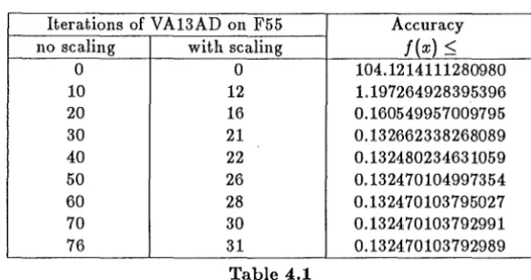
The next stage gave more interesting results because automatic scaling was introduced at every iteration in the modified code as described in Section 3.2 above. Analytic gradients were still used in the calculation of the search direction and the line search algorithm of VA13AD was unchanged. The effect of automatic scaling on VA13AD is considerable; the results of Table 4.1 show that more than twice as many iterations are required without automatic scaling for full accuracy in

f (

x"').

Iterations of VA13AD on F55 Accuracy

no scaling with scaling

f(x)

~

0 0 104.1214111280980

10 12 1.197264928395396

20 16 0.160549957009795

30 21 0.132662338268089

40 22 0.132480234631059

50 26 0.132470104997354

60 28 0.132470103795027

70 30 0.132470103792991

76 31 0.132470103792989

Table 4.1

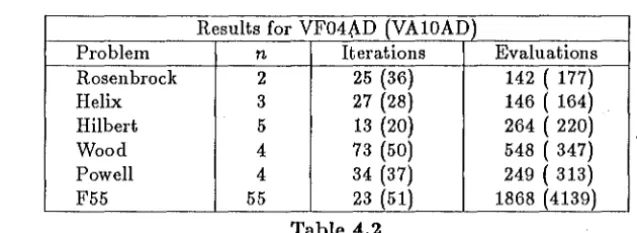
[image:10.600.150.443.397.551.2]

it should be remembered that, with automatic scaling, twice as much information is being used to modify the estimated second derivative information at each iteration. Of course, 2n extra function evaluations must be made at every iteration in order to estimate the second derivative information and we have already pointed out that this is wasteful unless these evaluations are necessarily made when estimating the first directional derivatives using formula (1.10). Therefore, the final stage in the construction of the new algorithm was to implement the remaining features as described in Section 3. The results on some standard (and well-known) test functions are presented in Table 4.2 which gives the number of iterations and evaluations of

f(x)

required to obtain an accuracy

f(x) - f(x*)

<

10-14_•

Results for VF04.{\D (VAlOAD)

Problem n Iterations Evaluations

Rosen bro ck 2 25 (36) 142 ( 177)

Helix 3 27 (28) 146 ( 164)

Hilbert 5 13 (20) 264 ( 220)

Wood 4 73 (50) 548 ( 347)

Powell 4 34 (37) 249 ( 313)

F55 55 23 (51) 1868 (4139)

Table 4.2

The Harwell library routine VAlOAD was also applied to the same test problems and results are included in parentheses in Table 4.2. VAlOAD is also a finite difference Quasi-Newton algorithm but second derivative information is represented by Choleski factors and sometimes the DFP updating scheme is used instead of the BFGS scheme [4]. This algorithm uses a more accurate line search than VF04AD and uses a different strategy to choose between forward and central difference formulae.

The results for Table 4.1 were obtained on the IBM 3084

Q

mainframe computer at Harwell and those in Table 4.2 were obtained on a SUN 3/160 micro-computer system at the author's own institution.

5. DISCUSSION

[image:11.602.131.450.316.432.2]

further investigation here. However, the results of the previous section show that even for the simplest of implementations the conjugate direction approach can give considerable advantages even on serial machines.

REFERENCES

[1] K. W. Brodlie, A.R. Gourlay, J. Greenstadt, Rank-one and rank-two corrections to positive definite matrices expressed in product form, J. Inst. Maths. Applies. 11 (1973), 73-82.

[2] C.G. Broyden, The convergence of a class of double rank minimization algorithms. 2. The new algorithm, J. Inst. Maths. Applies. 6 (1970), 222-231.

[3] W.C. Davidon, Optimally conditioned optimization algorithms without line searches, Math. Prog. 9 (1975), 1-30.

[4] R. Fletcher, A new approach to variable metric algorithms, Computer Journal 13 (1970), 317-322.

[5] D. Goldfarb, A family of variable metric methods derived by variational means, Maths of Comp. 24 (1970), 23-26.

[5a] D. Goldfarb and A. Idnani, A numerical stable dual method for solving strictly convex quadratic programs, Math. Prog. 27 (1983), 1-33.

[6]

S-P. Han, Optimization by updated conjugate subspaces, Report DAMTP 1985/NA9 (1985),

University of Cambridge.

[7] M.R. Osborne and M.A. Saunders, Descent methods for minimization, in "Optimization," Eds. R.S. Anderssen, L.S. Jennings, D.M. Ryan, University of Queensland Press, St Lucia, 1972, pp. 221-237.

[8] M.J.D. Powell, Updating conjugate directions by the BFGS formula, Report DAMTP 1985/NAll {1985), University of Cambridge.

[9] M.J.D. Powell, Subroutine VA1SAD, Harwell Subroutine Library (1975), U.K. Atomic Energy Research Establishment.

[to]

U. Schendel, "Introduction to numerical methods for parallel computers," Ellis Horwood,

Chichester, 1984.

[11]

D.F. Shanno, Conditioning of quasi-Newton methods for function minimization, Maths of

Comp. 24 {1970), 647-656.

Keyword.'l. conjugate directions, unconstrained optimization, BFGS, automatic scaling, finite differences, parallel pro-cessing.

1980 Mathematics subiect classifications:

APPENDIX

Test program used to validate VA13AD

DOUBLE PRECISION F,G,SCALE,W,X,XD,YD

COMMON /VA13BD/IPRINT,LP,MAXFUN,MODE,NFUN

COMMON/XXX/XD,YD

DIMENSION XD(61),YD(61),X(66),G(55),SCALE(66),W(1870)

EXTERNAL F55

DO 1 I=1,51

SCALE(I)=0.1DO

XD(I)=0.126664DO*DBLE(I-1)

YD(l)=SIN(XD(I))

1 X(I)=(1.0D0+0.5DO*YD(I))*XD(I)

DD 2 I=52,56

SCALE(I)=0.1DO

2 X(I)=O.ODO

IPRINT=1

MAXFUN=100

ACC=1.0D-14

CALL VA13AD(F65,66,X,F,G,SCALE,ACC,W)

STOP

END

SUBROUTINE F66(N,X,F,G)

DOUBLE PRECISION C,F,G,X,XD,YD

COMMON /XXX/ XD,YD

DIMENSION XD(51),YD(61),X(65),G(55)

F=O.ODO

DO 1 !=52,55

1 G

(I)

=O. ODO

DO 2 I=1,51

c~x(52)+X(I)*(X(53)+X(I)*(X(54)+X(I)*X(66)))-YD(I)

F=F+C*C+(X(I)-XD(I))**2

G(I)=2.0DO*

$

((X(63)+X(I)*(2.0DO*X(54)+3.0DO*X(I)*X(55)))*C+X(I)-XD(I))

DO 2 J=52,65

G(J)=G(J)+2.0DO*C

2 C=C*X(I)