Seismic Vulnerability Assessment from Earthquake Damages Historical Data Using Constrained Optimization Technique

(1)

ISSN Online: 2327-4344 ISSN Print: 2327-4336

DOI: 10.4236/gep.2018.62007 Feb. 28, 2018 89 Journal of Geoscience and Environment Protection

Seismic Vulnerability Assessment from

Earthquake Damages Historical Data Using

Constrained Optimization Technique

Abed Benaïchouche

1

_{, Caterina Negulescu}

1*

_{, Olivier Sedan}

1

_{, Zohra Boutaraa}

2

1_{BRGM (French Geological Survey), Orléans, France}

2_{Materials Sciences and Environment Laboratory, Hassiba Ben Bouali University of Chlef, Chlef, Algeria}

Abstract

This present work falls within the context of efforts that have been made over the past many years, aimed in improving the seismic vulnerability modelling of structures when using historical data. The historical data describe the in-tensity and the damages, but do not give information about the vulnerability, since only in the ’90 the concept of vulnerability classes was introduced through the EMS92 and EMS98 scales. Considering EMS98 definitions, RISK-UE project derived a method for physical damage estimation. It intro-duced an analytical equation as a function of an only one parameter (Vulne-rability Index), which correlates the seismic input, in term of Macroseismic Intensity, with the physical damage. In this study, we propose a methodology that uses optimization algorithms allowing a combination of theoretical-based with expert opinion-based assessment data. The objective of this combination is to estimate the optimal Vulnerability Index that fits the historical data, and hence, to give the minimum error in a seismic risk scenario. We apply the proposed methodology to the El Asnam earthquake (1980), but this approach remains general and can be extrapolated to any other region, and more, it can be applied to predictive studies (before each earthquake scenarios). The ma-thematical formulation gives choice for regarding, to the optic of minimizing the error, either for the: 1) very little damaged building (D0-D2 degree) or 2) highly damaged building (D4-D5 degree). These two different kinds of optics are adapted for the people who make organizational decisions as for mitiga-tion measures and urban planning in the first case and civil protecmitiga-tion and urgent action after a seismic event in the second case. The insight is used in the framework of seismic scenarios and offers advancing of damage estima-tion for the area in which no recent data, or either no data regarding vulne-rability, are available.

How to cite this paper: Benaïchouche, A., Negulescu, C., Sedan, O. and Boutaraa, Z. (2018) Seismic Vulnerability Assessment from Earthquake Damages Historical Data Using Constrained Optimization Tech-nique. Journal of Geoscience and Environ-ment Protection, 6, 89-111.

https://doi.org/10.4236/gep.2018.62007

Received: December 20, 2017 Accepted: February 25, 2018 Published: February 28, 2018

(2)

DOI: 10.4236/gep.2018.62007 90 Journal of Geoscience and Environment Protection

Keywords

Seismic Damage Scenario, Damage Database, Vulnerability Assessment, Inverse Optimization, Model Calibration, El Asnam Earthquake, RISK-UE

1. Introduction

Optimization algorithms have started to be widely used in the field of earth-quake engineering because of their capability to calibrate the model when no data are available for important parameters associated to behavior of the system (e.g. a system can be a building, a bridge, a network…). The first utilization of the optimization algorithms has been at the scale of one structure generally for fitting the model parameters (e.g. as the Young modulus, reinforcement bar di-ameter, compression resistance…). Several studies have also focused on effective computational methods of cost optimization for bridges [1] [2] [3] and struc-tures in general [4]. Recently, [5] used optimization process for the design of structures. The application of the framework proposed by them is illustrated in a bridge design optimization problem where the column reinforcement bar di-ameter and concrete cover are considered as design pardi-ameters. [6] presents a hybrid optimization methodology for the probabilistic finite element model up-dating of structural systems. In paper [6], the model updating process is formu-lated as an inverse problem, analyzed by Bayesian inference, and solved using a hybrid optimization algorithm.

Even if the optimization process is widely used at the scale of one structure, it is less common to apply it at the scale of a group of buildings, networks or the scale of town analysis. More recently, the optimization algorithms were also used for the natural hazard studies at large scales, and more particularly, for manage the decision after the catastrophic event. [7] proposes a simulation model to find out optimum evacuation routes, during a tsunami using Ant Colony Optimiza-tion (ACO) algorithms. [8] proposes a framework that clarifies the interrela-tionships between notions of coping capacity, preparedness, robustness, flexibil-ity, recovery capacflexibil-ity, and resilience, previously espoused as independent meas-ures, and provides a single mathematical decision problem for quantifying these measures congruously and maximizing their values. [9] proposes a fuzzy mul-ti-criteria model to deal with “qualitative” (unquantifiable or linguistic) or in-complete information and illustrates it within the post-earthquake reconstruc-tion problem in Central Taiwan, including the restorareconstruc-tion concerning the safe and serviceable operation of “lifeline” systems, such as electricity, water, and transportation networks, immediately after a severe earthquake.

(3)

on this subject, which demonstrate the demand of stakeholders and first res-ponders (e.g. civil protection) to have a better understanding and evaluation of damages and the various outcomes from these kind of studies. Different metho-dologies are applied for the assessment of the earthquake damages, which are generally based on two mandatory terms: the level of hazard and the level of vulnerability of the exposure (i.e. element at the risk). A very complete state of art of the development of seismic vulnerability assessment methodologies for va-riable geographical scales over the past 30 years is presented in [14]. Different methodologies are facing over the years: the widest used methodologies based on a vulnerability index [15] [16] [17] [18]; pushover-based vulnerability analysis

[19]; displacement-based vulnerability assessment procedure [20] and buildings’ vulnerability assessment using the parameter less scale of seismic intensity [21].

[22] [23] provide a detailed description (Summary of Software, Methodology, IT Details, Exposure Module, Hazard Module, Vulnerability Module and Output) of the existing software for seismic risk assessment that is either open source or has been made available to the GEM Risk Team. Here we are dealing with em-pirical methodologies based on the vulnerability index obtained from observa-tional data after earthquakes events. These methods are very useful for the re-presentation of the vulnerability at large scale (see [13] for more details of the used methodology).

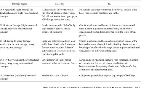
Concerning empirical methods, starting from the first “Earthquake damage probability matrices” derived by [24] after the saint Fernando earthquake and presented to the “Fifth World conference on earthquake engineering”, all the empirical methods for assessment of the seismic damage of structure are based on the relation between the observed intensity and the observed damage. One key moment in the collecting and the utilisation of the Earthquake damage data is the development of the European Macroseismic Scale—EMS98 [25] which is the first intensity scale that clearly defines the concept of vulnerability. Table 1

gives the classification of damage in EMS98 according to masonry and rein-forced concrete buildings. Before this scale, the previous scales Mercalli-Cancani Sieberg Scale—MCS [26], Modified Mercalli scale (MM-31 and MM-56) [27]

(4)

[image:4.595.62.539.87.383.2]

Table 1. Classification of damage to masonry and reinforced concrete buildings (according to EMS98).

Damage degree Masonry RC

D1 Negligible to slight damage (no structural damage, slight non-structural damage)

Hairline cracks in very few walls. Fall of small pieces of plaster only. Fall of loose stones from upper parts of buildings in very few cases.

Fine cracks in plaster over frame members or in walls at the base. Fine cracks in partitions and infills.

D2 Moderate damage (slight structural damage, moderate non-structural damage)

Cracks in many walls. Fall of fairly large pieces of plaster. Partial collapse of chimneys.

Cracks in columns and beams of frames and in structural walls. Cracks in partition and infill walls; fall of brittle cladding and plaster. Falling mortar from the joints of wall panels.

D3 Substantial to heavy damage (moderate structural damage, heavy non-structural damage)

Large and extensive cracks in most walls. Roof tiles detach. Chimneys fracture at the roofline; failure of individual non-structural elements (partitions, gable walls).

Cracks in columns and beam column joints of frames at the base and at joints of coupled walls. Spalling of concrete cover, buckling of reinforced rods. Large cracks in partition and infill walls, failure of individual infill panels.

D4 Very heavy damage (heavy structural damage, very heavy non-structural damage)

Serious failure of walls; partial

structural failure of roofs and floors. Large cracks in structural elements with compression failure of concrete and fracture of rebars; bond failure of beam-reinforced bars; tilting of columns. Collapse of a few columns or of a single upper floor.

D5 Destruction (very heavy structural

damage) Total or near total collapse Collapse of ground floor or parts (e.g. wings) of buildings.

framework of some European Commission projects, but their accessibility, espe-cially to original “raw” data, is fastidious.

[32] systematically compared statistical modelling techniques for different empirical datasets and explored many of the issues raised regarding the treat-ment of uncertainty.

Database typologies and their typical issues depend on the manner on which the observations were obtained they were been obtained: for Detailed “Engi-neering” Surveys and Surveys by Reconnaissance Teams the main issue is the possibility of unrepresentative samples; for the Rapid Surveys methods, generally the evaluation concern the habitability or the safety not the evaluation of the damage; while for remotely sensed survey method, which is quite new and not already able to efficiently evaluate other damage degrees than the collapse or very heavy damage [33]. For all these cases it is quite rare to have the three es-sential terms at the scale of the building or census block: intensity measure, building typology, and hence it vulnerability, and damage degree. Moreover, once this “original/unchanged” dataset is defined, usually data manipulation and combination were done in order to associated to some related parameters and develop new method for vulnerability assessment.

(5)

the best vulnerability index and its characteristics to be use in the seismic risk scenarios using optimization procedure.

2. Historical Case Study and Available Observed Data on

Damages

A retro-scenario of the October 10, 1980 El Asnam earthquake was performed by the authors [34] [35] using Armagedom tools [13] developed by the French Geological Survey (BRGM). In this paper, we are just using the intensity and damage observations in order to find the vulnerability index that will give the smaller error between the observed damage and the damages calculated numer-ically with Armagedom software.

Chlef city (formerly named El Asnam) situated 200 km west of the capital of Algeria Algiers, is an area that suffers of important seismic activities due to the interaction of the two Eurasian and African plates. Major earthquakes rocked the city during the last century, the last event that caused major damages being the one of October 10, 1980; known as El Asnam earthquake and killed around 3000 persons. This event was qualified as the largest earthquake ever known in the west-Mediterranean region. Different international studies [36] [37] [38]

[image:5.595.258.490.458.661.2]

were performed based, or in collaboration, with the Algerian Technical Inspec-tion of ConstrucInspec-tion (CTC) that conducted a large field investigaInspec-tion and dam-age inventory in El Asnam city on 5131 buildings. Figure 1 presents the ten sec-tors in which the city was divided after the CTC’s survey (adapted from [37]). Based on this data, [36] established a buildings damage classification, in which the damage levels are: Green—very little damage. Can be occupied immediately; Orange: needs further study before it can be either occupied or condemned; Red:

(6)

[image:6.595.208.539.130.351.2]

Table 2. Damage classification of El-Asnam buildings by [36]. ID: district Id. I: EMS98 intensity. Ntot: total number of buildings in percentage. Gr: green damage grade (D0 to D2). Or: orange damage grade (D3). Re: red damage grade (D4 to D5). Un: undefined damage grade.

ID I Damage classification

Gr (%) OR (%) Re (%) Un (%)

1 IX 19.08 60.24 20.49 0.17

2 IX 31.11 45.55 22.22 1.11

3 IX 21.53 45.03 33.28 0.13

4 IX 37.89 38.28 23.82 0.00

5 IX 31.92 36.88 31.19 0.00

6 IX 44.50 35.16 18.19 1.14

7 IX 46.93 38.48 11.07 3.49

8 IX 42.50 42.77 10.89 3.81

9 IX 27.75 49.59 20.20 2.44

10 IX 38.02 28.38 33.59 0.00

Total 33.48 42.06 23.39 1.07

condemned and should be demolished. Table 2 presents the number of build-ings and the damage classification (number of red, orange and green) performed by [36] in each of the ten sectors of the city. The seismic vulnerability assessment of the existing buildings has never been done either.

The data given in Table 2 represents the collected observational dataset. This representation of information is the very common for post-earthquake damages assessment after seismic event. This concern ancient’s earthquake as well as the most recent earthquake (Aquila 2009), for which intuitively we can imagine to have more detailed information’s, but in reality, this is not the case.

3. Model Calibration

3.1. Model Description

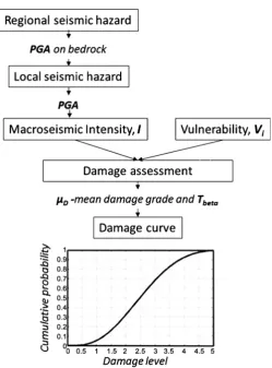
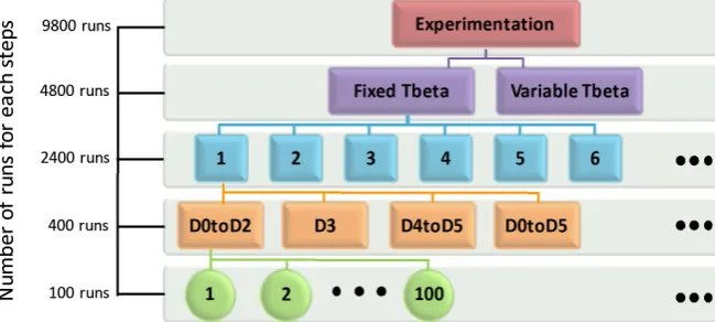
Figure 2 schematize the general methodology for seismic damage calculation. It presents each of the most important phases necessary for creating an earthquake scenario: regional seismic hazard, local seismic hazard, etc. In the case of El As-nam, the hazard modules (module 1, 2 and 3) are not performed, since we got the observed macroseismic intensity. Here all performed simulations (9800 runs) were executed on the Armagedom tools [13] developed by the French Geological Survey (BRGM) and used for simulation of the damage scenarios.

(7)

[image:7.595.251.501.63.401.2]

Figure 2. General methodology and modulus in Armagedom software for seismic dam-age calculation.

highly vulnerable). Depending on the buildings proprieties (materials, age of construction, height…), these last are regrouped in categories; commonly known as typologies (see [40] for more details). Therefore, a value of Vi is

as-signed to each building typology. For each typology, the mean damage degree (µD: between zero and five) is estimated based on a vulnerability function:

6.25 13.1 2.5 1 tan i D

I V

h

µ

φ

  + ⋅ − 

= ⋅ +_ _ __

 

 

(1)

I represent the seismic hazard described in terms of macroseismic intensity (EMS98 scale), Vi the vulnerability index, and φ the ductility index, which is

evaluated taking into account the building typology and its constructive features ([39]); it controls the slope of the curves and assumes different values to fit the data obtained through damage surveys. For residential buildings, it takes a value of 2.3.

Finally, the damage distribution is derived using beta probability density function (Equation (2)) and the beta cumulative density function (Equation (3)).

( )

₍

₎

(

) (

)

(

)

1 1

1 Γ

Γ( ) Γ

r t r

t

t x a b x

P x

r t r b a

β

− − −

−

− ⋅ −

= ⋅

(8)

( )

a

( )

x

P_β x =

∫

P_β

ε

⋅d

ε

(3)

With 𝑎𝑎 < 𝑥𝑥 < 𝑏𝑏 and

(

3 2

)

0.007 D 0.052 D 0.287 D

r=t µ − µ + µ . The parameters a,

b, t, and r are the parameters of the distribution and Γ is the gamma function. The parameter r is the variance and controls the shape of the distribution.

The parameter t (named after Tbeta) resulting from the probability calculation

by the law β determines the dispersion of the values; it therefore represents the propagation of uncertainties that can come from different sources as the input data, or the variable behaviour of the same typology structure to the seismic ha-zard. In the Risk-EU method, this one is fixed to t = 8 which represent the best fits for the European buildings [40]. However, the study posits to leave it varia-ble in a range of values, hence the optimal value for each typology can be found numerically.

In order to use the beta distribution, it is necessary to refer to the damage grades Dk (k = 0 to 5) defined by EMS scale; for this purpose, it is advisable to

assign value 0 to the parameter a and value 6 to the parameter b [18].

The outcome is the distribution in terms of the six levels defined in EMS98: D0 (undamaged), D1 (slight damage), D2 (moderate damage), D3 (heavy dam-age), D4 (partial collapse) and D5 (total collapse) for each location that is sepa-rately considered, given by the equation (Equation (4)).

(

k

)

1

( )

P D≥D = −P_β k (4)

To perform seismic damage scenarios, very often, many typologies of build-ings exist in the same studying area. Therefore, to run the simulation model (Armagedom software) we need to describe:

• _{the total number of typologies;}

• _{the vulnerability indices (}_V_i_{) and}_T_beta_{parameters for each typology;} • _{the spatial distribution of the typologies in each district (polygon) of the}

af-fected area vulnerability (nbBat).

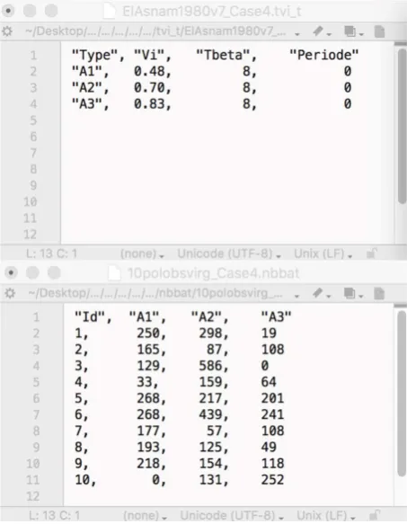
In Armagedom software, these parameters are stored in file (*.txt) as follows:

• _the_V_i_and_T_beta_{are regrouped in the same file (}_{Figure 3}_{) called *.tvi_t. The}

file is structured in four columns;

• _{type of building as character, vulnerability index as float,}_T_beta_{parameters as}

float and period as float. Each line represents a specific typology;

• _{the nbBat are stocked in another file (}_{Figure 3}_{) called *.nbbat. This file is}

given as table in which, each line represents the area, the number of columns represent the number of typology and the value the number of buildings. Examples of *.nbbat and *.tvi_t files for the case with three typologies (A1, A2, A3) are illustrated in Figure 3.

3.2. Vulnerability Assessment Using Inverse Optimization

(9)

[image:9.595.260.487.71.363.2]

Figure 3. Required file for Armagedom software for the case with three typologies (A1, A2, A3): top—the *.tvi_t file containing the vulnerability index Vi and bottom—the

*.nbbat file containing the distribution of the typologies in each polygon.

damages to the observed ones?” This question is the main issue for all the seis-mic risk analysis either produced for prediction without a situation of seisseis-mic event or produced in quasi-real time situation during a seismic crisis.

The observed data in Table 2 give two major information:

i) the macroseismic EMS98 intensity, which is uniform (IX) for all the city; ii) the observed damages, regrouped on three classes: green (regroups D0, D1 and D2), orange (represents D3) and red (regroups D4 and D5).

Our problem is clearly considered underdetermined (for number of typologies higher than 1) because there is fewer equations than unknowns. Here, the total number of parameters needed to run the model depends on the total number of typology. Therefore, for 𝑁𝑁PQRS the number of parameters to determine is

(

)

PQRS PQRS V WC

2×N + N − 1 ×N _< . Therefore, for this ill-posed problem, the

opti-mization algorithm leads to local solutions. This limitation, often problematic for solving optimization problem is very interesting for us. Where, not only one final solution is obtained but all solutions minimizing the objective function are retained. The final decision comes to the expert to choose/validate the most ap-propriate one.

(10)

exam-DOI: 10.4236/gep.2018.62007 98 Journal of Geoscience and Environment Protection

ples of questions than can be answered by experts:

• _{What error needs to be reduced?}

1) Uniform error on all damage degree D0 to D5;

2) Error on D4 to D5 damage, useful for civil protection in case of seismic ca-tastrophe;

3) Error on D0 to D2 damage, useful for mitigation and planning.

• _{Which parameters can be fixed?}

1) Number of typology and its corresponding Vi and Tbeta;

2) The nbBat parameters; repartition of number of buildings per typology in each area.

• _{Which parameter can be constrained?}

1) Number of typology between 1 and 6;

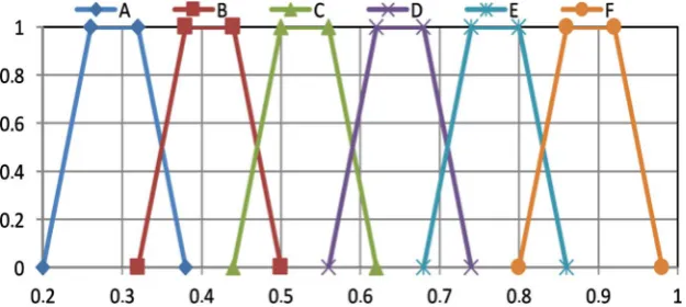
2) Values of Vi, not varying from 0 to 1 but constrained by the fuzzy function

(Risk-UE) method (Figure 4); 3) Tbeta between 4 and 16.

In our study, we have explored a large number of solution in order to evaluate the impact of expert’s constraints on the final solutions. Finally, validate the most appropriate one. We underline that, the range of variation of the vulnera-bility index is governed by the fuzzy function method (Figure 4), which adapt with the number of typologies [18] [40] [41].

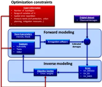
For our simulations, we used Armagedom for the forward modelling and the augmented Lagrange multiplier method described in [42] for the inverse one.

Figure 5 illustrate the conceptual scheme followed for solving the problem. The proposed methodology was implemented in R programming language and environment [43] using the SOLNP algorithm available in “Rsolnp” package

[44]. This process was repeated 100 times to generate 100 values of Vi, Tbetaand

[image:10.595.218.531.547.687.2]

nbBat values. These solutions represent potential solution, which will be ana-lyzed by the expert in order to select the most appropriate one. We will show in the next section, that all the 100 solutions present a very little difference. The algo-rithmic parameters used are as follows: population size = 50, generations = 200, crossover fraction = 0.8, and stall generations = 100. In fitting convex function

(11)

[image:11.595.207.538.69.352.2]

Figure 5. Conceptual scheme for optimization process.

models for the data, we use ellipsoidal, super-ellipsoidal, and Nataf transforma-tion based methods.

For each observed damage grade, we compute the misfit error between ob-served and estimated damage (Equation (5)). In order to have a uniform distri-buted damage grade error for all polygons we define for each damage grade the entity defined in Equation (6). Finally, the objective function to minimize can be defined as a weighted sum of the theses entities (Equation (7)).

0 1 2

3

4 5

D D D 0 1 2 0 1 2 0 1 2

D 3 3 3

D D 4 5 4 5 4 5

D D D D D D D D D

D D D

D D D D D D

Est Obs Obs

E E E = − = −   =  −   

(5)

(

)

(

)

( )

(

)

(

)

0 1 2 0 1 2 0 1 2

3 3 3

4 5 4 5 4 5

1 D D D D D D D D D

2 D D D

3 D D D D D D

ˆ max min ˆ max min ˆ max min

J E E E

= − + =     − + = − +  

(6)

1 1 2 21 3 3

J=ω ⋅ +J ω ⋅J +ω ⋅J

(7)

The choice of the weights ω ω ω1, 2, 3 depends on the application and should

be fixed by the expert. For example, for people who make organizational deci-sions J1 must be important for them, therefore ω1 should be greater than ω2

and ω3. In the other hand for civil protection and urgent action after a seismic

(12)

In this study, we have tested 4 hypotheses:

1) Case 1: error on D4 to D5 useful for civil protection in case of seismic ca-tastrophe; in this case, we take

(

ω ω ω1, 2, 3

) (

= 0.01, 0.0 ,1 1 .

)

2) Case 2: error on the damage degree D0 to D2, useful for mitigation and planning; in this case, we take

(

ω ω ω1, 2, 3

) (

= 1, 0.01,0 0. 1 .

)

3) Case 3: error on damage degree D3 the most complicated to evaluate; in this case, we take

(

ω ω ω1, 2, 3

) (

= 0.01,1,0 0. 1 .

)

4) Case 4: uniform error on all damage degree; in this case, we take

(

ω ω ω1, 2, 3

) (

= 1 ,,1 1 .

)

Figure 6 illustrates the organigram of explored solutions.

The number of simulations runs needed was determined in order that pro-viding stable predictions for numerical results. The choice of 100 was guided by two raisons:

-The variability of 100 estimated Vi indices values is very low. This is shown in

section 4 (Figure 8(a1) and Figure 8(a2)).

-We first execute 10, 20, 50 then 100 model runs during the experimentation phase. We clearly observe that first (mean) and second (variance) moment-order for 50 and 100 models run were similar. As optimization process is not time-consuming process, we fix to number of model runs to 100.

4. Results and Comments

In this section, we present a synthetic analysis of obtained results. We remember that our main objective here, is the determination of optimal vulnerabilities pa-rameters (Vi, Tbeta and nbBat) fitting at best the historical observed damages. The

[image:12.595.210.535.551.697.2]

originality of the method relies on practical and operational aspects. Indeed, the method gives a panel of optimal solutions (ill-posed problem), and final choice return experts. For clarity of exposition, we will first present the typical results obtained for a specific hypothesis (here case 4; uniform distributed error for all damages) and for a fixed number of typologies (here 4 typologies). Then, syn-thetic results for two cases (from D0 to D2 in Figure 9 and, from D4 to D5 in

Figure 8) of all executed simulations (2400 for each case).

(13)

Figure 7 represents an example of obtained results for a number of typologies fixed to 4 for the case 4. The optimization process provides 100 possible solu-tions to experts for the vulnerability index (Figure 7(a)), the Tbeta parameters

(Figure 7(b)) and nbBat to choose/validate the most appropriate one. In Figure 7(a) (respectively Figure 7(b)), different colors (blue, green, red and black col-or) of the points represent vulnerability index (respectively Tbeta) for the 4

typol-ogies. Its show that:

• _V_i_{’s values are very close even the variation range are very high (fuzzy}

func-tion in Figure 4). For example, blue points (first typology) in Figure 7(a)

gives values of Vi around 0.8 and can take values between 0.785 and 0.965. • _{Even if, the values of V}_i_{present a small variability, the value of T}_beta

parame-ter (Figure 7(b)) have a high dispersion (between 4 and 16).

Figure 7(c) and Figure 7(d) present the errors on the number of structures given in the number and in percentage for two arbitrary solutions (samples 17 and 61). The barplots presents the error on the damages degree D0 to D2 (green color), D3 (orange color) and D4 to D5 (red color) for the 10 districts. It shows that the distribution is very different for the two case, in the other hand the error

Figure 7. Mathematical solutions for the vulnerability parameters (Vi and Tbeta) for case 1

(

ω1=1,ω2=1,ω3=1

)

with 4 typolo-gies: (a) 100 possible solutions for Vi; (b) 100 possible solutions for Tbeta; (c) Damages errors on the number of buildings

(14)

remains distributed uniformly. This can be explained by the fact that the prob-lem is ill posed and infinity of local minima are possible, and very different solu-tion can satisfy the same optimizasolu-tion criteria. However, this limitasolu-tion is very interesting in our study, were experts must validate the optimal solution. These results emphasise the idea of global consideration of results, by looking to the error at the scale of the city and in all the districts of the studied area. Looking separately at a zoomed area the interpretation of results can be inexact, since, for example for the solution 17, for the district five the error is very reduced, and vice versa, for example for the district one of the solution 61.

In follow, we will present the obtained results for two practical cases.

• _{The first one, very useful for crisis management. Where, the authority is}

in-terested by the number of highly damaged buildings; here named as D4 to D5. All other categories, remains less important in this case.

• _{The second one, very useful for mitigation and planning. Where, concerned}

authority need information about habitability.

For each case presented below, we have executed 2400 simulations in order to test some hypothesis and it allows to answer to two important questions:

1) Does higher number of typologies implies lower misfit error?

2) In the Risk-UE method, Tbeta parameter was calibrated according to the

European buildings and fixed to 8. So, changing its value improves the accuracy of the model predictions?

4.1. Case1: Crisis Management

In this section, we will summarize the obtained results for the 2400 executed si-mulations. In Figure 8, the graphics in the left column show results for fixed Tbeta

parameters (equal to 8) according to the European buildings, and the right one for optimal Tbeta. We present the results for the three sets of observational

dam-ages grade described below (D0 to D2, D3, D4 to D5).

In Figure 8(a1) and Figure 8(a2), boxplots represent results for possible val-ue for vulnerability indices (y-axis) for each number of typologies (x-axis). Each boxplot contains 100 values. We observe that the variability of Vi indices values

is very low for the two cases; fixed and optimal Tbeta. In Figure 8(a1) for one

ty-pology, the Vi value is always the same because the optimization process

con-verges for the global minimum. In this specific case, the well-posed problem has a unique solution, which is Vi equal to 0.70; Tbeta is fixed to 8 and nbBat is equal

to total number of buildings.

In Figure 8(b1) and Figure 8(b2), boxplots represent results for possible val-ue for Tbeta parameters (y-axis) for each number of typologies (x-axis). Each

boxplot contains 100 values. In Figure 8(b1), all Tbeta values are equal to 8

be-cause it is fixed input parameter; the graphic plotted only to show for comparison with Figure 8(b2). This last, show clearly that for all number of typologies, the Tbeta

(15)

[image:15.595.54.539.47.647.2]

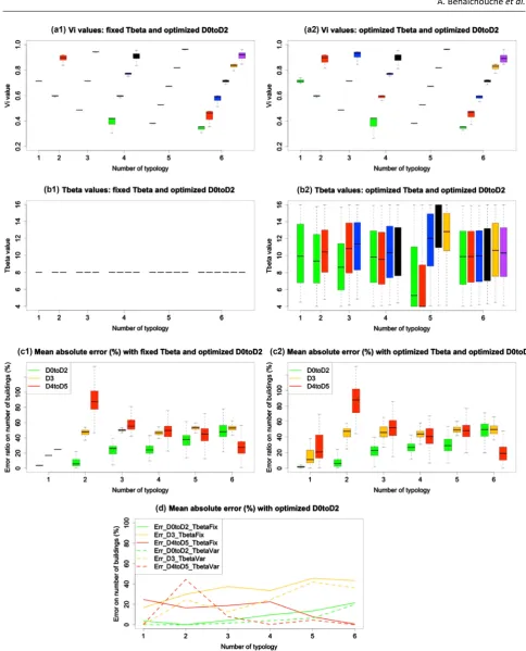
Figure 8. Results for crisis management case: (a1) the value of Vi indices for different typologies with fixed Tbeta, (a2) the value of

Vi indices for different typologies with optimal Tbeta, (b1) the value of Tbeta parameters for different typologies with fixed Tbeta, (b2)

the value of Tbeta parameters for different typologies with optimal Tbeta, (c1) the mean absolute error in percentage for different

typologies with fixed Tbeta, (c2) the mean absolute error in percentage for different typologies with optimal Tbeta, (d) Comparison

(16)

absolute error (y-axis) for each number of typologies (x-axis). Each boxplot contains 100 values. Here, we have compare the results for three indicators: mean absolute error on D0 to D2 (green), on D3 (orange) and on D4 to D5 (red). We remember that here, we are minimizing according to high weight on D4 to D5. Therefore, we expect a best performance on D4 to D5 (red) and less on the other one. The two graphics Figure 8(c1) and Figure 8(c2) confirm that error on D4 to D5 is very small (less than 10%) for the 2 cases; with fixed and optimal Tbeta comparing to the error on D3 and D4 to D5.

Figure 8(d) reports the lowers band in Figure 8(c1) (continues lines) et Fig-ure 8(c2) (dashed lines) in the same graphics. Each plot represents the mini-mum error (among the 100) for the considered indicator for each number of ty-pologies. Bottom and top of the boxplot in Figure 8 are the 25th_{and 75}th

percen-tile, the ban near the middle of the box is the median and the ends of the whisk-ers are the minimum and maximum. This graphics allows the comparison be-tween the two cases (fixed and optimal Tbeta).

We observe that for:

• _{D4 to D5 indicator that for fixed and optimal T}_beta_{the misfit error on D4 to}

D5 is less than 2%, except for the case with one typology. Moreover, the in-crease of the number of typologies does not improve the model’s results. This can be explained by the fact that increasing a number of typologies, the Vi

index have more constraints for variation range given by the fuzzy function. And the second one that Tbeta fixed to 8 was accurately calibrated in the

Risk-UE project [15] and it is representative of European buildings.

• _{D0 to D2 and D3 indicators, we show that considering T}_beta_{variable and}

in-creasing the number of typologies reduce the misfit error (up to 20%). How-ever, it’s meaningless because, the optimization criterion is highly weighted on D4 to D5.

For El Asnam area, for the crisis management situation, after the analysis of the mathematical solutions, we suggest to use for the predictive damage scenario five or six typologies, with the Vi equal to the values presented in the Figure 4

and the Tbeta fix equal to 8. The variation of the Tbeta do not ameliorate the results

and the use of less typologies give less information for the same error (less than 2%). The choice of the expert is constantly balanced between the acceptable er-ror and the needed information. In the case of El Asnam, if we are looking only to the D4 to D5 damages, as is generally the case for crisis management, we pre-fer to choose more typologies (that will represent better the geographical distri-bution of the damage) for the same error. However, if for one reason, we are also interested by D3 damages, in this case the error increase at around 30% for five typologies and hence, we recommend using two typologies for which the error is less than 10%.

4.2. Case 2: Mitigation and Planning

(17)

[image:17.595.55.540.38.650.2]

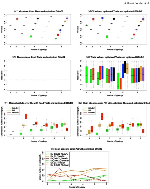
Figure 9. Results for mitigation and planning case: (a1) the value of Vi indices for different typologies with fixed Tbeta, (a2) the

value of Vi indices for different typologies with optimal Tbeta, (b1) the value of Tbeta parameters for different typologies with fixed

Tbeta, (b2) the value of Tbeta parameters for different typologies with optimal Tbeta, (c1) the mean absolute error in percentage for

different typologies with fixed Tbeta, (c2) the mean absolute error in percentage for different typologies with optimal Tbeta and (d)

(18)

same manner as Figure 8. In Figure 9(a1) and Figure 9(a2), boxplots represent results for possible value for vulnerability index (y-axis) for each number of ty-pologies (x-axis). Each boxplot contains 100 values. We observe that minor dif-ferences in the Vi indices value variability exist for the two cases; fixed and

op-timal Tbeta. In Figure 9(a1) for 1, 3 or 5 typologies, the Vi value always converge

to a global minimum. This is very specific to study case and cannot be genera-lized. The same analysis can be reported in Figure 9(a2) for 5 typologies.

In Figure 9(b1) and Figure 9(b2), boxplots represent results for possible val-ue for Tbeta parameters (y-axis) for each number of typologies (x-axis). The same

analysis can be done here as in Figure 9(b1) et Figure 9(b2); the values of Tbeta

parameters are highly dispersive.

In Figure 9(c1) and Figure 9(c2), boxplots represent results for mean abso-lute error (y-axis) for each number of typologies (x-axis). Each boxplot contains 100 values. Here, we have compare the results for three indicators: mean abso-lute error on D0 to D2 (green), on D3 (orange) and on D4 to D5 (red). We re-member that we are minimizing with high weight on D0 to D2. Therefore, we expect a best performance on D0 to D2 (green) and less on the other one. The two graphics seems giving equivalent results in order of magnitude for D0 to D2 errors. In addition, we observe that this error grow with the increase of the number of typologies.

Figure 9(d) reports the lowers band in Figure 9(c1) (continues lines) and

Figure 9(c2) (dashed lines). Each plot represents the minimum error (among the 100) for the considered indicator for each number of typologies. This graph-ics allows the comparison between the two cases (fixed and optimal Tbeta). We

observe that:

• _{For D0 to D2 indicator that for fixed and optimal T}_beta_{the misfit error on D0}

to D2 is less than 20%. We observe that the increase of the number of typolo-gies increase the misfit error. This can be explained by the fact that increasing a number of typologies, the Vi index have more constraints for variation

range given by the fuzzy function. And the second one that Tbeta fixed to 8

was accurately calibrated in the Risk-UE project (Mouroux et al., 2004) and it is representative of European buildings.

• _{For D0 to D2 and D3 indicators, we show that considering T}_beta_{variable and}

increasing the number of typologies reduce the misfit error (up to 2%) for D4 to D5 indicator. We also notice, that, for 2 typologies the result for D4 to D5 indicators with fixed Tbeta is better than with optimal one. These results

de-pend on the study case and it’s meaningless to extrapolate the results except for D0 to D2 indicator in this case.

For El Asnam area, for the mitigation and planning situation, after the analy-sis of the mathematical solutions, we suggest to use for the predictive damage scenario two typologies, with the Vi equal to (0.6 and 0.87) and the Tbeta fix equal

(19)

ame-DOI: 10.4236/gep.2018.62007 107 Journal of Geoscience and Environment Protection

liorate the results (from Figure 9(d). we can see that the error is quite stable for 3, 4 and 5 typologies with optimal Tbeta, but increase for the same number of

ty-pologies with Tbeta fixed to 8).

In Figure 9, the bottom and top of the boxplot are the 25th_{and 75}th_percentile,

the ban near the middle of the box is the median and the ends of the whiskers are the minimum and maximum. From the results of the two cases, we can de-duce that the methodology is calibrated for table the important damage degrees, that can be managed by the optimization process as can be noticed in the Figure 8(d), where the error is less than 2% for any number of typology. This is more hardly to manage for the error relative to the case 2: mitigation and planning, for which, the error, although stable for 1, 2 and 3 typologies, grow up for the situa-tions with 4, 5 and 6 typologies.

The fact that we use different typologies introduces more error, but that also gives supplementary information relative to the location of the damages. If the question of the user is just to know the total error without knowing the distribu-tion by districts, in this case the use of only one typology can be useful. However, generally, even in crises management situation, in addition to this question, the second question is the identification of the most affected districts in order to send the rescue. In this case, the geographical description of the error is re-quired.

5. Conclusions

We have aimed in this work to develop unified computational method for as-sessment of vulnerability of structures, to be used for seismic risk scenarios at the town scale, when the underlying uncertainties are modelled using random variables, interval analysis, and (or) fuzzy variables. The developed approach is based on the minimization of the error between observed and estimated damag-es and it allows the determination of the number of typologidamag-es classdamag-es, the damag- esti-mation of their vulnerability index and associated Tbeta value as well as the spatial

distribution in the studied area (nbBat). This method remains general and can be applied for any observed dataset, for which generally the information related to the typologies and their vulnerability are not available. The main insights after the analysis of the results are:

• _{The Risk-EU methodology and the model that it proposed fit very well the}

damages D4 to D5. When the attention is played to the damages D0 to D2 the estimation is correct but damage D3 remains the most difficult to be as-sessing because the diagnosis experts on this category remain very subjective and the description remains very vague.

• _{The results of our work corroborate the affirmation on the Risk-EU}

metho-dology, where the Tbeta was fixed equal to 8, based on the statistic treatments

(20)

variability on the results and the choice of Tbeta = 8 must be respected. • _{Contrary to the expectance, increasing the number of typologies does not}

reduce the error for the results. Indeed, the fact of constraining by the expert the Vi by the fuzzy function restricts the search space. Therefore, the total

error is increased but, by increasing the number of typologies, the geographic description of the vulnerability in the studied area is improved and brings supplementary needed information (e.g. the hierarchizing of the most dam-aged areas).

The two cases (crisis management and planning and mitigation) have two different trends response: i) for mitigation case, increasing the number of typol-ogy increases the misfit error; ii) on the other hand in the case of crisis manage-ment increasing the number of typology improves the model prediction. In some cases, the optimization algorithm can detect the number of classes that minimize the error, that means on one hand that, a smaller number of classes are insufficient (small number of degree of freedom), and on the other hand that, spending time for dividing and refining the number of classes is useless. In the case of El Asnam situation, the optimum number of typologies was not clearly identified. The mathematical formulation of the objective function gives the opportunity to have a perfect fit of the vulnerability parameters (error that tends to zero) by minimizing the error for a specific damage grade (e.g. a mini-mization related to D4 to D5 damage gives the most accurate vulnerability pa-rameters for civil protection for urgent action after a seismic event). Hence, the approach can answer to different actors that work at the scale of the town in dif-ferent situations (e.g. planning, mitigation action, retrofitting, crises manage-ment). Of course, the total error (total number of building as a sum of building in each area) is much less big than the error related to each area. This observa-tion should be considered in the studies in which only the total error is com-puted, which have certainly big utilities in certain almost “real time crises situa-tion” when the first question is the rough estimate of number of victims; but quickly after, the spatial localization of damages is asked, in order to know where to send the first aids, and hence the error at the area level become very impor-tant. The method that we propose presents a better integration of the vulnerabil-ity and loss results could allow cvulnerabil-ity councils or regional authorities to plan in-terventions based on a global view of the site under analysis, leading to more accurate and comprehensive risk mitigation strategies that support the require-ments of safety and emergency planning.

References

[1] Adeli, H. and Ge, Y. (1989) A Dynamic Programming Method for Analysis of Bridges under Multiple Moving Loads. International Journal for Numerical Me-thods in Engineering, 28, 1265-1282.https://doi.org/10.1002/nme.1620280604 [2] Adeli, H. and Mak, K.Y. (1990) Interactive Optimization of Plate Girder Bridges

Subjected to Moving Loads. Computer-Aided Design, 22, 368-376.

(21)

DOI: 10.4236/gep.2018.62007 109 Journal of Geoscience and Environment Protection [3] Sirca Jr., G.F. and Adeli, H. (2005) Cost Optimization of Prestressed Concrete

Bridges. Journal of Structural Engineering, 131, 380-388.

https://doi.org/10.1061/(ASCE)0733-9445(2005)131:3(380)

[4] Adeli, H. and Balasubramanyam, K.V. (1988) Expert Systems for Structural Design: A New Generation. Prentice Hall, Upper Saddle River.

[5] Bisadi, V. and Padgett, J.E. (2015) Explicit Time-Dependent Multi-Hazard Cost Analysis Based on Parameterized Demand Models for the Optimum Design of Bridge Structures. Computer-Aided Civil and Infrastructure Engineering, 30, 541-554.https://doi.org/10.1111/mice.12131

[6] Sun, H. and Betti, R. (2015) A Hybrid Optimization Algorithm with Bayesian Infe-rence for Probabilistic Model Updating. Computer-Aided Civil and Infrastructure Engineering, 30, 602-619.https://doi.org/10.1111/mice.12142

[7] Forcael, E., González, V., Orozco, F., Vargas, S., Pantoja, A. and Moscoso, P. (2014) Ant Colony Optimization Model for Tsunamis Evacuation Routes. Comput-er-Aided Civil and Infrastructure Engineering, 29, 723-737.

https://doi.org/10.1111/mice.12113

[8] Faturechi, R. and Miller-Hooks, E. (2014) A Mathematical Framework for Quanti-fying and Optimizing Protective Actions for Civil Infrastructure Systems. Comput-er-Aided Civil and Infrastructure Engineering, 29, 572-589.

[9] Opricovic, S. and Tzeng, G.H. (2002) Multicriteria Planning of Post-Earthquake Sustainable Reconstruction. Computer-Aided Civil and Infrastructure Engineering, 17, 211-220.https://doi.org/10.1111/1467-8667.00269

[10] Strasser, F.O., Bommer, J.J., Şeşetyan, K., Erdik, M., Çağnan, Z., Irizarry, J., Crow-ley, H., et al. (2008) A Comparative Study of European Earthquake Loss Estimation Tools for a Scenario in Istanbul. Journal of Earthquake Engineering, 12, 246-256. https://doi.org/10.1080/13632460802014188

[11] Molina, S., Lang, D.H. and Lindholm, C.D. (2010) SELENA—An Open-Source Tool for Seismic Risk and Loss Assessment using a Logic Tree Computation Procedure.

Computers & Geosciences, 36, 257-269.https://doi.org/10.1016/j.cageo.2009.07.006 [12] Hancilar, U., Tuzun, C., Yenidogan, C. and Erdik, M. (2010) ELER Software—A

New Tool for Urban Earthquake Loss Assessment. Natural Hazards and Earth Sys-tem Sciences, 10, 2677-2696.https://doi.org/10.5194/nhess-10-2677-2010

[13] Sedan, O., Negulescu, C., Terrier, M., Roullé, A., Winter, T. and Bertil, D. (2013) Armagedom—A Tool for Seismic Risk Assessment Illustrated with Applications.

Journal of Earthquake Engineering, 17, 253-281.

https://doi.org/10.1080/13632469.2012.726604

[14] Calvi, G.M., Pinho, R., Magenes, G., Bommer, J.J., Restrepo-Vélez, L.F. and Crow-ley, H. (2006) Development of Seismic Vulnerability Assessment Methodologies over the Past 30 Years. ISET Journal of Earthquake Technology, 43, 75-104. [15] Mouroux, P., Bertrand, E., Bour, M., Le Brun, B., Depinois, S. and Masure, P. (2004)

The European RISK-UE Project: An Advanced Approach to Earthquake Risk Sce-narios. The 13th World Conference on Earthquake Engineering, Vancouver, 1-6 August 2004, Paper No. 3329.

[16] Petrini, V. (1993) Rischio sismico di edifici pubblici, Parte I Aspetti metodologici. GNDT-CNR Report, Tipografia Moderna.

[17] HAZUS99, F.E.M.A. (1999) Earthquake Loss Estimation Methodology: User’s Ma-nual. Federal Emergency Management Agency, Washington DC.

(22)

DOI: 10.4236/gep.2018.62007 110 Journal of Geoscience and Environment Protection Seismic Risk Analysis. PhD Thesis.

[19] Borzi, B., Pinho, R. and Crowley, H. (2008) Simplified Pushover-Based Vulnerabili-ty Analysis for Large-Scale Assessment of RC Buildings. Engineering Structures, 30, 804-820.https://doi.org/10.1016/j.engstruct.2007.05.021

[20] Crowley, H., Pinho, R. and Bommer, J.J. (2004) A Probabilistic Displacement-Based Vulnerability Assessment Procedure for Earthquake Loss Estimation. Bulletin of Earthquake Engineering, 2, 173-219.https://doi.org/10.1007/s10518-004-2290-8 [21] Orsini, G. (1999) A Model for Buildings’ Vulnerability Assessment using the

Para-meterless Scale of Seismic Intensity (PSI). Earthquake Spectra, 15, 463-483.

https://doi.org/10.1193/1.1586053

[22] Crowley, H., Colombi, M., Crempien, J., Erduran, E., Lopez, M., Liu, H., Milanesi, M., et al. (2010) GEM1 Seismic Risk Report: Part 1. Technical Report, GEM Foun-dation, Pavia, 5.

[23] Crowley, H., Colombi, M., Crempien, J., Erduran, E., Lopez, M., Liu, H., Milanesi, M., et al. (2010) GEM1 Seismic Risk Report: Part 2. Technical Report, GEM Foun-dation, Pavia, 5.

[24] Whitman, R.V., Reed, J.W. and Hong, S.T. (1973) Earthquake Damage Probability Matrices. In: Proceedings of the 5th World Conference on Earthquake Engineering, Vol. 2, Palazzo DEI CONGRESSI (EUR), Rome, 2531-2540.

[25] Grunthal, G. (1998) European Macroseismic Scale 1998. Cahiers du centre Européen de Géodynamique et de Séismologie, 15, 1-99.

[26] Sieberg, A. (1930) Geologie der Erdbeben. Handbuch der Geophysik, 2, 552-555. [27] Wood, H.O. and Neumann, F. (1931) Modified Mercalli Intensity Scale of 1931.

Bulletin of the Seismological Society of America, 21, 277-283.

[28] Medvedev, S.V., Spohneuer, W. and Karnik, V. (1965) Seismic Intensity Scale Ver-sion MSK 1964. Akad. Nauk SSSR, Geofiz. Kom., 10. (In Moscow)

[29] Colombi, M., Borzi, B., Crowley, H., Onida, M., Meroni, F. and Pinho, R. (2008) Deriving Vulnerability Curves Using Italian Earthquake Damage Data. Bulletin of Earthquake Engineering, 6, 485-504.https://doi.org/10.1007/s10518-008-9073-6 [30] Lambert, J., Levret-Albaret, A., Cushing, M. and Durouchoux, C. (1996) Mille ans

de séismes en France. Ouest Editions, Nantes, 79.

[31] SisFrance (2005) Catalogue des séismes français métropolitains, BRGM, EDF, IRSN.

http://www.sisfrance.net

[32] Rossetto, T., Ioannou, I. and Grant, D.N. (2013) Existing Empirical Fragility and Vulnerability Functions: Compendium and Guide for Selection. GEM Technical Report, GEM Foundation, Pavia, 65.

[33] Rossetto, T., Ioannou, I., Grant, D.N. and Maqsood, T. (2014) Guidelines for the Empirical Vulnerability Assessment. GEM Technical Report, GEM Foundation, Pa-via, 65.

[34] Boutaraa, Z., Negulescu, C., Arab, A. and Sedan, O. (2018) Buildings Vulnerability Assessment and Damage Seismic Scenarios at Urban Scale: Application to Chlef City (Algeria). KSCE Journal of Civil Engineering.

[35] Boutaraa, Z., Negulescu, C., Arab, A. and Sedan, O. (2015) Scénarios de risque sismique pour la ville de Chlef (Ex El Asnam) Algérie. 9eme Colloque AFPS, Marne la vallée. (In French)

(23)

DOI: 10.4236/gep.2018.62007 111 Journal of Geoscience and Environment Protection Strengthening of Damaged Buildings in the Region of El Asnam: Engineering Ge-ology, Geotechnical and Geophysical Characteristics of the Town of El Asnam and Other Sites. Report IZIIS, 82-55.

[37] Bertero, V.V. and Shah, H.C. (1983) El-Asnam Algeria Earthquake Oktober 10, 1980: A Reconnaissance and Engineering Report. EERI.

[38] EERI, Database of Concrete Buildings Damaged in Earthquakes.

https://www.eeri.org/2013/11/onlinedatabase-of-concrete-buildings-damaged-in-ea

rthquakes/

[39] Lagomarsino, S. and Giovinazzi, S. (2006) Macroseismic and Mechanical Models for the Vulnerability and Damage Assessment of Current Buildings. Bulletin of Earth-quake Engineering, 4, 415-443.https://doi.org/10.1007/s10518-006-9024-z

[40] Milutinovic, Z.V. and Trendafiloski, G.S. (2003) Risk-UE An Advanced Approach to Earthquake Risk Scenarios with Applications to Different European Towns. Contract: EVK4-CT-2000-00014, WP4: Vulnerability of Current Buildings.

[41] Demartinos, K. and Dritsos, S. (2006) First-Level Pre-Earthquake Assessment of Buildings using Fuzzy Logic. Earthquake Spectra, 22, 865-885.

https://doi.org/10.1193/1.2358176

[42] Ye, Y. (1987) Interior Algorithms for Linear, Quadratic, and Linearly Constrained Non-Linear Programming. PhD Thesis, Department of ESS, Stanford University, Stanford.

[43] Team, R.C. (2015) R: A Language and Environment for Statistical Computing. R Foundation for Statistical Computing, Vienna.