University of Warwick institutional repository: http://go.warwick.ac.uk/wrap
A Thesis Submitted for the Degree of PhD at the University of Warwick
http://go.warwick.ac.uk/wrap/35769
This thesis is made available online and is protected by original copyright.
Please scroll down to view the document itself.
Polyphonic Audio Analysis
Edward R. S. Pearson B.Sc.
Department of Computer Science
A thesis submitted to
The University of Warwick
for the degree of
Doctor of Philosophy
Contents
1 Introduction 2
1.1 Artificial Hearing 2
1.2 The human auditory system 3
1.3 Objectives of this work 6
1.4 Automated Transcription 7
1.5 Previous Work 11
1.6 Mathematical Notation 12
1.7 Equipment Used 13
1.8 Thesis Organisation 13
2 Representations of Audio Signals 17
2.1 Introduction 17
2.2 Some commonly used representations 18
2.2.1 Linear Transforms 19
2.2.2 Non-Linear Transforms 23
2.2.3 Multiscale Techniques 24
2.3 The Multiresolution Fourier Transform 27
2.3.1 Linearity and Invertibility 27
2.3.4 Representation Requirements 40
2.3.5 MET Definition and Properties 41
2.3.6 Oversampled Transform 46
2.3.7 Inverse Transform 46
2.3.8 MFT Interpretation 47
2.3.9 Summary 48
3 MFT Implementation and Initial Results 49
3.1 Introduction 49
3.2 Selecting the MET Parameters 49
3.3 MFT Implementation 60
3.3.1 Analysis Vector Generation 60
3.3.2 Forward Transform Implementation 61
3.3.3 Inverse Transform Implementation 66
3.4 Some Examples 68
3.4.1 Introduction 68
3.4.2 A Simple Sinusoid 68
3.4.3 A complex tone 70
3.4.4 A Violin Note 72
3.5 Summary 72
4 A Model of Note Structure 74
4.1 Introduction 74
CONTENTS iii
4.2.1 Note Structure 75
4.2.2 Note Juxtaposition 76
4.2.3 Other Signal Features 79
4.3 A Feature Hierarchy 80
4.4 A Signal Model 82
4.4.1 Notes 83
4.4.2 Partials 84
4.5 Summary 89
5 Feature Detection 91
5.1 Detection Overview 91
5.2 Feature Detection 92
5.2.1 Partial detection 95
5.2.2 Partial Onset Detection 97
6 Transcription 106
6.1 Introduction 106
6.2 Transcription Data Structures 108
6.2.1 Partial Bank 109
6.2.2 Partials 109
6.2.3 Note Bank 111
6.2.4 Note Hypotheses 111
6.2.5 Accepted Note List 112
6.3 Transcription Algorithms 113
6.3.1 Generating Onset Events 113
6.3.5 Note-bank iteration 120
7 Results 123
7.1 Introduction 123
7.2 Phase Differencing 124
7.3 Two Piano Notes 126
7.3.1 The MFT Levels 126
7.3.2 Feature Detection 130
7.3.3 Multiresolution Processing 135
7.4 Bach Woodwind Trio 140
7.5 Schubert Piano Trio 146
7.6 Summary 149
8 Conclusions 151
8.1 Thesis Summary 151
8.1.1 Signal Representation 151
8.1.2 Signal Modelling and Analysis 152
8.1.3 Transcription 155
8.2 Concluding Remarks 157
List of Figures
1.1 The Human Auditory System as an Information Hierarchy 4
1.2 Magnitude of Two Piano Note Audio Signal 7
1.3 Score for Two Piano Note Signal 15
1.4 Magnitude of Fourier Transform of Two Piano Note Signal 15 1.5 A combined time-frequency representation of two piano notes 16
2.1 Wavelet Transform Lattice 26
2.2 Idealised representation of a two-feature signal 29
2.3 Finite resolution representation 30
2.4 Inappropriate representation 31
2.5 I Va (t, 0.7)1 (Infinite resolution) 32
2.6 IV.(to, 0-)1 (Scale 1) 33
2.7 I Va(to,0-01 (Scale 2) 34
2.8 I Vb (t, w ) I (Infmite resolution) 35
2.9 IVb(to, w)I(Scale 1) 35
2.10 IVb(to , 0-)1 (Scale 2) 36
2.11 117,(t, co) I (Infinite resolution) 37
2.12 1-d MFT structure 43
3.3 Analysis vectors (freq), a = 1 55
3.4 Analysis vectors (time),
a =
1 563.5 Analysis vectors (freq),
a =
2 563.6 Analysis vectors (time),
a =
2 573.7 Level tessellation, a = 1 57
3.8 Level tessellation, a = 2 58
3.9 Non-relaxed mFr synthesis vector (freq) 59
3.10 Non-relaxed mFr synthesis vector (time) 59
3.11 Analysis-Synthesis window products (frequency) 60
3.12 Algorithm for Efficient FPSS Generation 62
3.13 Forward Transform Implementation 64
3.14 'Blocked' Forward Transform Implementation 67
3.15 'Blocked' Forward Transform Window 68
3.16 'Blocked' Inverse Transform Implementation 69
3.17 4 Mn' levels of a sinusoidal tone 70
3.18 4 Mn' levels of a complex tone 71
3.19 4 Mn' levels of a violin note 72
4.1 Partial Meshing 78
4.2 Partial Coincidence 78
4.3 The Feature Hierarchy 82
4.4 Typical Synthesiser Envelope Model 85
LIST OF FIGURES vii
5.2 Piano note (C4) onset at MFT level 9 98
5.3 Piano note (C4) onset at MFT level 12 99
5.4 Violin note (C4) onset at MFT level 9 100
5.5 Violin note (C4) onset at MV!' level 12 101
6.1 Transcription Data Structure Hierarchy 108
7.1 Violin note showing forward phase-difference 124
7.2 Polar and magnitude only plots of tone with changing frequency 125
7.3 Two Piano Notes: MFT level 9, magnitude 127
7.4 Two Piano Notes: MFT level 10, magnitude 127
7.5 Two Piano Notes: MFT level 11, magnitude 128
7.6 Two Piano Notes: MFT level 12, magnitude 128
7.7 Two Piano Notes: mFT level 13, magnitude 129
7.8 Two Piano Notes: CC ik (9), magnitude 130
7.9 Two Piano Notes: c(11), magnitude 131
7.10 Two Piano Notes: CC ik (13), magnitude 131
7.11 Two Piano Notes: onset events, level 9 133
7.12 Two Piano Notes: onset events, level 10 133
7.13 Two Piano Notes: onset events, level 11 134
7.14 Two Piano Notes: onset events, level 12 134
7.15 Two Piano Notes: onset events, level 13 135
7.16 Two Piano Notes: Combined onset events, no transient detector 136 7.17 Two Piano Notes: Combined onset events, with transient detector 137
7.18 Two Piano Notes: Partial Positions 138
7.22 Bach Trio: level 11 magnitude 142
7.23 Bach Trio: level 13 magnitude 142
7.24 Bach Trio: onset events, level 9 143
7.25 Bach Trio: onset events, level 11 143
7.26 Bach Trio: onset events, level 13 144
7.27 Bach Trio: partials with tracking levels 145
7.28 Bach Trio: note allocation and partial positions 145
7.29 Schubert Trio: partials with tracking levels 147
7.30 Schubert Trio: note allocation and partial positions 148
Acknowledgements
This work was supported by UK SERC and Solid State Logic Ltd. It was conducted within the Image and Signal Processing Group in the Department of Computer Science at The University of Warwick, UK.
Many people have contributed to this work, in particular, the staff and students of the department. Special thanks goes to Jeff Smith, Rod Moore and Roger Packwood who gave invaluable software support and assistance with hardware construction.
Great thanks must go to my friends and colleagues for their stimulation and support — Abhir Bhalerao, Andrew Calway, Simon Clippingdale, Roddy McColl, Andrew Davies, Hayley Ryder, Martin Todd, Philip Underdown, June Wong, the members of Warwick University Caving Club and many others.
I am particularly indebted to my supervisor, Dr. Roland Wilson. Without his great knowledge, understanding and unending stream of ideas, this work would not have been possible.
Finally I would like to thank my mother for her endless love, support and patience, Catherine for giving me the inspiration to carry on when times were hard and Cho for making a dream come true.
Introduction
1.1 Artificial Hearing
Many people listen to, or at least hear, some form of music almost every day of their lives. However, only some of the processes involved in creating the sensations and emotions evoked by the music are understood in any detail. The problem of unravelling these processes has been much less thoroughly investigated than the comparable topics of speech and image recognition; this has almost certainly been caused by the existence of a greater number of applications awaiting this knowledge. Nevertheless, the area of music perception has attracted some attention over the last few decades and there is an increasing interest in the subject largely arising from the availability of suitably powerful technology. It is becoming feasible to use such technology to construct artificial hearing devices which attempt to reproduce the functionality of the human auditory system. The construction of such devices is both a powerful method of verifying operational theories of the human auditory system and may ultimately provide a means of analysing music in more detail than man. In addition to the analytical benefits, techniques developed in this manner are readily applicable to the creative aspects of music, such as the composition of new music and musical sounds.
CHAPTER 1. INTRODUCTION 3
1.2 The human auditory system
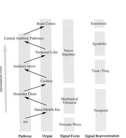
The human auditory system extends from the outer ear (pinna) through a complex and highly sensitive set of mechanical and chemo-electrical systems to the temporal lobe of the brain. The physical layout is normally divided into the outer, middle and inner ears; the auditory nerve and central auditory pathways. The ear itself, a highly complex system comprising many delicate components, not only serves to convert sound waves in the atmosphere to nerve impulses but also includes the sensory organs of balance. Though the processing performed by the ear on the acoustic signal has been the subject of a long, and sometimes heated, debate, it is now generally accepted that it operates as both a temporal and frequency analyser. The inner ear performs the conversion from mechanical vibrations to nerve impulses by means of the cochlea, a spiral tube divided in two along its length by the basilar membrane. The tube becomes smaller in diameter along its length so that, as sound waves pass along it, different frequencies resonate in different regions and excite tiny hair cells on the membrane. At low frequencies at least, these hair cells can respond fast enough to respond synchronously with the extreme excursions of the signal. This topic is the best documented area of hearing, having a large body of work associated with it, see [Ge18 1] or [Nor70] for thorough surveys. After the cochlea, the signal passes into the auditory nerve and our degree of knowledge of the physical aspects of its subsequent processing and interpretation starts to decrease fairly rapidly. Experimentation by many workers has, however, suggested the qualities of the signal which are measured and the types of features recognised by the subsequent processing stages.
Brain Cortex Emotional
Central Auditory Pathways
Symbolic
obe
Impulses
•
Auditory nerve
Ossicular Chain
Outer/Middle Ear
Time /
FreqMechanical Vibration
Temporal
Air
Pressure Wave
[image:14.595.108.523.172.628.2]Pathway Organ Signal Form Signal Representation
CHAPTER 1. INTRODUCTION 5
'events', some are perceived as having a distinct pitch and are commonly referred to as notes. The number of properties which may be attributed to notes, as demonstrated by the richness of language used to describe them, is vast. For the purposes of analysis, however, only four are typically discussed, namely: pitch, loudness, duration and timbre. In the case where a single note has been isolated, pitch and loudness are primarily functions of the frequency and amplitude of the signal, respectively. Duration is fairly simply related to the physical duration of the signal, though exactly which facets of the signal correspond to timbre is largely unknown. Part of this problem is that the term is fairly loosely defined; W. Dixon Ward in [Nor70] says that the term has become a 'wastebasket' category, "if two sounds are 'different' though having the same pitch and loudness, then they must differ in timbre". Classical (now obsolete) theory speculates that this quality is related to the spectral distribution of the note; while certainly contributing, the simple experiment of observing the great difference in timbre of playing a sound backwards, via a tape machine, suggests that temporal aspects of the signal also play an important role. J. M. Grey in [Gre75] devised a timbral space in which the distance between two points corresponded to the perceived difference in timbre between two notes. However, the space was produced by a multi-dimensional scaling algorithm run on the results of a set of listening tests and so, unfortunately, the relationships between the axes of the space and any physical attributes of the test signals could not be deduced.
hence the term virtual pitch. Many thorough surveys are available on this subject including [Sma70] and [Ge181], while a more musical look at the topic can be found in [War70].
Notes can be broken down into a set of partials, each a pseudo-sinusoidal function having a single frequency. For a note to have a clear pitch of N Hz. the partials with the largest magnitudes have frequencies of N Hz, 2N Hz, 3NHz. etc. These partials are normally referred to as the harmonics of the note, the others sometimes being referred to as the inharmonic partials. As the relative magnitude of the harmonics decreases with respect to the inharmonic-partials the pitch of the tone becomes decreasingly distinct. The tones produced by bells have inharmonic-partials with significant magnitude. For the notes analysed in this work, it is assumed that the magnitude of the inharmonic-partials is so small that they can be ignored. For this reason, the terms harmonic and partial are used interchangeably.
1.3 Objectives of this work
The work described in this thesis leads to a system which can interpret a limited set of signals and produce output at the level of symbols which correspond to the notes of a score. The term automatic transcription system 1 has become applied to such such systems, since the symbolic
representation produced is similar to the information represented on a musical score and the process can be considered equivalent to writing down the score on hearing a piece of music.
The main objectives of this work are:
1. Investigate some aspects of the nature of musical signals in the context of signal processing and pattern recognition.
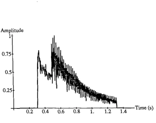
0.2 0.4 0.6 0.8 1. Amplitude
1-0.75
0.5
0.25
Time (s) 1.2 1.4
CHAPTER / . INTRODUCTION 7
2. Develop a signal representation suited to the analysis of musical signals.
3. Devise analytical techniques which make the best use of the devised representation.
4. Build an example application using the representation and the techniques in order to assess their potential.
1.4 Automated Transcription
In order to move towards a methodology for building an automatic transcription system, the problem is first discussed in general terms.
[image:17.595.163.426.424.632.2]Figure 1.2 shows the magnitude of a short segment of a musical signal with respect to time. Figure 1.3, which is the musical score which would have been performed in order to produce the
signal.
Figure 1.2: Magnitude of Two Piano Note Audio Signal
Figure 1.3: Score for Two Piano Note Signal
horizontal scale to measure time but represents frequency or pitch on its vertical scale; which is a far more perceptually important parameter of the music than its magnitude with time. In addition, the durations of the notes are represented by the form of the symbols used.
A note can be thought of as a special kind of sound, though it is not possible to define the precise point at which a sound becomes a note. Both are experienced as a single percept, but that described as a note, by a typical listener, will have a definite pitch associated with it as well as a clear starting time and, often less distinctly, a finishing time. A listener could judge which of two sounds started first but could only attempt to place them above or below each other in pitch if they were notes.
A simple working definition of the task to be implemented by a music transcription system can now be proposed:
Definition 1.1 The requirement of an automatic music transcription system is to produce a 'score-like' representation of a piece of music given only a description of the amplitude of its acoustic
signal with respect to time.
The minimum information required in the output data consists of estimates of the onset time, frequency and duration of each of the notes in the signal.
The techniques developed in this work are specifically aimed at polyphonic signals. A poly-phonic, rather than monopoly-phonic, signal is one where more than one note occurs simultaneously. Typically the classification is based on the number of instruments playing and how many notes they
Amplitude 1
0.75
0.5
0.25
500 1000 1500 2000 2500 300 eq (Hz)
CHAPTER 1. INTRODUCTION 9
Figure 1.4: Magnitude of Fourier Transform of Two Piano Note Signal
not restricted to the number of notes it can play at once; it is polyphonic. From a signal processing point of view, the situation is not quite as clear. The simple two note signal presented above would probably be classified as monophonic since only one note is 'played' at any time, however the first note is still decaying when the second starts (legato), and so must be considered polyphonic for the purposes of signal analysis. Much previous work has been applied to monophonic sources. While not without value, the techniques developed are often dependent on this monophonicity and so can never be applied in polyphonic situations. The work presented here has tried to avoid such limitations.
note, the signal is the sum of two component signals which would have to be separated from each other before such analysis could take place. Such separation of a signal into a set of component signals is know as signal segmentation; to perform this on a given class of signals requires the definition of a segmentation strategy which has been discussed in general terms by several authors including Harlick [Har83] Wilson and Spann [WS87b]. The deduction of a such a strategy for music transcription forms the basis of Chapter 4.
The problem of not having an explicit frequency scale for the raw data can be approached by applying some transform to the data which results in an alternative representation of it. This is discussed at length in the next chapter; for now observe Figure 1.4, which is the magnitude of the Fourier Transform (Fr) of the signal. This representation has axes displaying frequency and
amplitude. Clear peaks can be seen corresponding to the harmonics or partials of the notes. The frequencies of the notes could be obtained from these peaks but notice that there exists the problem that the harmonics are intermingled and need to be assigned to notes which is, again, a signal segmentation problem. However, the more fundamental problem with this form of the signal is that there is now no time axis; it is therefore no more use for deducing all of the parameters of the notes than Figure 1.2, since it is impossible to observe either the onset times or durations of the notes.
CHAPTER 1. INTRODUCTION 11
of ridges grouped by onset time. Each note corresponds to one of these sets. The first set of ridges (toward the front) is more widely spaced than the second, corresponding to the pitch of the first note being higher than the second. The basic parameters of the music can now be observed directly from the signal representation. There are clearly two sets of partials, they occur at different times and the first is higher in frequency than the second. The argument here, all be it fairly heuristic, is simply that this kind of time-frequency representation is clearly more suited to the analysis of musical signals than a representation describing it exclusively in terms of time or frequency. For these reasons, it has become a standard technique to use time-frequency representations (with the Short-time Fourier Transform being the most common) for the analysis of audio and many other signals. Various forms of time-frequency representations and their relative merits are discussed in Chapter 2.
1.5 Previous Work
CHAPTER 1. INTRODUCTION 13
Work by Charles Watson in [Wat86], using a variety of heuristic techniques, obtained accurate results from synthesised and natural signals. The algorithms developed need to be tailored interac-tively to suit the characteristics of the particular signal being analysed, it is not clear whether they could be generalised to cope automatically with a range of input signals.
A variety of techniques have been described by Chafe et al in [CMR82, CJK + 85] and [SS86] from the Centre for Computer Research in Music and Acoustics (CCRMA). These techniques have been used as tools forming part of an interactive signal editor, but it is not known if they have, to date, been successfully integrated into a fully-automated analysis system.
Of particular interest is a recent work by Serra [Ser89], though being oriented towards sound manipulation and resynthesis rather than transcription, it does demonstrate the power gained by using a feature based analysis method. Very briefly, the system generated a pseudosinusoidal expansion of the signal using a short-time Fourier transform. The representation could then be used to drive an additive synthesiser, the output of which could be combined with the residual of the original to produce realistic reconstructions. The system is oriented towards monophonic sound sources but can cope with the kind of 'overlap' polyphony described above. The user is required to know some of the parameters of the music as it is necessary to enter these before the analysis is performed. There is also an interactive stage after the automatic analysis when the accuracy of the partial tracks detected can be improved by the user.
vocal tract [RDP87], most notably as part of the CHANT project [Rod84, RPB84]. The models used
in this thesis are simple by comparison though there is no fundamental reason why more complex models could not be used within the analysis framework presented. The limitations of the signal model used are discussed in the final Chapter.
1.6 Mathematical Notation
The mathematical notation used in this thesis makes use of a great many superscripts and subscripts. In order to aid the reader, an attempt has been made to use this notation in a consistent manner. A particular letter is associated with each value to be represented e.g. t for a time. The letter is emboldened when it represents a vector e.g. t might be a vector of times. Elements of such vectors are referenced using a subscript e.g. for a single dimensional vector, ti would be the ith element of t. Elements of multidimensional vectors are referenced by means of a comma separated list of subscripts.
CHAPTER I. INTRODUCTION 15
1.7 Equipment Used
The experimentation and software development for this work was performed on several Sun Mi-crosystems computers. Analogue to digital and digital to analogue conversion of the audio signals was via equipment kindly supplied by Solid State Logic Limited of Oxford, U.K. who also partly funded the work. A sampling precision of 16 bits and a sampling rate of 48kHz was used for all signals. Test signals were synthesised using the CSound package from MIT, while natural sound sources were provided by the McGill University Master Samples Compact Discs and a variety of other prerecorded sources.
1.8 Thesis Organisation
Representations of Audio Signals
2.1 Introduction
This chapter comprises two main parts. After a brief discussion, there is a review of several signal representations which have been applied to the analysis of audio signals: the next section then introduces and defines the multiresolution Fourier transform (mFr) which forms the basis of the work presented in the subsequent chapters.
It is important to distinguish between a signal and a representation of that signal. The repre-sentation can be considered to be a view of the signal by some observer. A given signal may have many representations: many different views of the same data. For one dimensional signals, such as audio, the most common representation is that given by observing the signal in the time domain — other representations can be obtained by applying some signal transform. Different representations can give highly dissimilar views: some aspects of the signal may be revealed in one representation and hidden in another, as was demonstrated in Chapter 1.
Any system which processes audio signals must represent those signals internally in one or more ways. Simple systems which only perform modifications on an audio signal (e.g. an equaliser), may only use only the time domain description: the modifications they make are easily implemented
CHAPTER 2. REPRESENTATIONS OF AUDIO SIGNALS 17
in the time domain. An audio analysis system, which produces a symbolic output, rather than a modified signal, typically transforms the signal from the time domain into some more suitable representation, on which it then operates. The suitability of the representation depends upon the goals of the system. Where those goals are to produce a perceptually relevant set of symbols from the input signal, then it can be seen that the algorithms that the system must implement will be simplified by allowing them to operate on a signal representation which describes the signal in similar terms to those in which it is perceived. This similarity is of particular importance in an interactive analysis-synthesis system [CMR82, Ser89] where the transformed signal may be directly observed and possibly modified by the user. As was discussed in the previous chapter, it is generally agreed that the best representation for this type of work is one which incorporates aspects of both time and frequency and these are commonly referred to as combined or conjoint [Dau88b] representations.
2.2 Some commonly used representations
A wide variety of time-frequency representations have been investigated by many different workers and, as a result, there has been much literature published on the subject. Several comprehensive sur-veys of the topic have been published; a most exhaustive review has recently been given by [Coh89]
as a linear combination of signals,
v(t) = E kivi(t) (2.1)
1=1
where ki are constants, then its transform G(v) satisfies
G(v(t))
=
E kiqvi(t)) (2.2)1.1
The transform of the composite signal is the sum of the appropriately weighted transforms of the component signals. Equation 2.1 is a suitable model for musical signals, which, typically, consist of individual sounds 'mixed' together. A linear transform ensures that this form is retained in the transformed domain, clearly simplifying any analysis system based on it.
The Fourier Transform
The single most important transform in signal processing is the Fourier transform (Fr) which relates the time and frequency domains. The Fourier transform V(w) of a signal v(t) is defined by
V(w) = 1:v(t)e —.iw t dt (2.3)
The inverse transform is then defined as
lroo
V(t) = V(w)e3w t dco (2.4)
A similar transform can be defined for discrete signals and is referred to as the discrete Fourier transform (DFr).
(2.7)
(2.8)
CHAPTER 2. REPRESENTATIONS OF AUDIO SIGNALS 19
The Short Time Fourier Transform
The short time Fourier transform (STFT) is often called the 'phase vocoder' in speech [Por76] and music applications [Moo78, Can80]. The name arises from the fact that the transform coefficients are complex; previous vocoders had not included phase information.
The forward transform is defined as [Por80] 00
V2(t, co) = h(t — r)v(r)e-3"dr (2.5)
—00
The function h(t) is the analysis window and is chosen to be concentrated in both time and frequency. It is this localisation which means that V2(t, w) can be considered as a representation intermediate between v(t) and V(w). It can be seen from the STFT definition that it is a linear transform.
An inverse swr can be defined. The original signal can be recovered using [Por80]
cx)
v(t) f (t — 7-)v2(T,w)eiw t dr dt (2.6)
-00 -CO
The function f(t) is the synthesis window which, to ensure invertibility, must be related to the analysis window h(t) by
[00
h(t)f(—t)dt = 1
I -00
A discrete form of the STFT can be defined [Por80]. Given a time sequence, x(n), then
co
X2 (n,m) h(nR —
:=-00 0 < m < M
The indices n and m select the transform coefficients from a two-dimensional integral lattice covering the time-frequency plane. .R and 271M are the sampling intervals in time and frequency respectively.
As for the continuous case, with appropriate choices of sampling intervals and windows, this form of the transform is invertible [Por80].
M-1 00
1
x(n) =
-E
Ef
M , (n — m)X2(m,k)e3Tc4
•27r km sc=0 m=-00
E
f(n — sR)h(sR — n pM) = 5(p) (2.10)8=-00
for all n
Note that the representation has no redundancy when R = M.
The coefficients of the discrete STFT are best interpreted by considering rows and columns of
the representation individually. A single column, X 2 (no, m), can, from Equation 2.9, be seen to be the DFT of the time windowed signal h(noR — n)x(n). A single row is then a time sequence of
coefficients, one from each column, with m = mo.
00
X2 (n, mo) =
E
h(nR — (2.11)i=-00
which can be considered in terms of a convolution,
X2 (n, mo) = h(nR) * (x(nR)e rnonR ) (2.12)
This may be interpreted as the output of an analysis filter h(n) operating on a frequency shifted version of x(n) [Por801.
The summation limits in Equation 2.9 are given as ±oo, but in practice they depend on the analysis window, which is typically zero-valued outside some finite interval. This leads to the idea that efficient implementations of the STFT are possible using the fast Fourier transform (F,H) [Por76]
and this is the technique normally used in audio analysis [Moo78]. More recently, multirate filter bank implementations [SB87] have been used, which permit the application of quadrature mirror filter (QMF) techniques [ECG76]. Such a scheme removes aliasing in the analysis stage allowing the original signal to be perfectly reconstructed simply and efficiently.
CHAPTER 2. REPRESENTATIONS OF AUDIO SIGNALS 21
merits are not considered here. Note, however, that the Kaiser window [E74] is commonly used, e.g. [Ser89].
The Gabor Representation
Gabor (1947) did not agree with the prevailing idea that hearing was well represented by frequency based Fourier analysis, though the representation he proposed [Gab46] has more recently been
shown to be related to the STFT [Bas81]. Gabor stated "...it is our most elementary experience that
sound has a time pattern as well as a frequency pattern...". The Gabor representation is defined as an expansion of the signal
00
v (t) = E iai(t)
k,1=-oo
Cgk (2.13)
where Cm are the expansion coefficients and the basis functions, g ki (t) are time-frequency shifted versions of a Gaussian window g(t) = e.
gia(t) = g(t — kT)ej(int+0) (2.14)
TC2 = (2.15)
where T, 1, a and are all constants. Given the time and frequency dispersions of the basis functions and the sampling intervals T and LI, each transform coefficient Cki represents a region (Gabor called it a logon') of the time-frequency plane of size T x F, at time kT and frequency 1F. A drawback of the representation is that the basis functions g ki(t) are not orthogonal and so calculation of the expansion coefficients, Cki, is not straightforward, requiring either vast computa-tional resources or some iterative approximation. Recent work has lead to more efficient techniques [Bas81] but these are still computationally expensive compared to FFr based implementations of the
and frequency. This arises from Heisenberg's uncertainty principle [Pap77] which had previously been applied to quantum mechanics, but has become a fundamental result in signal processing. The principle implies that the time t and frequency f of some phenomenon cannot be measured simultaneously with arbitrary accuracy. The phenomenon must be considered to be somewhat dispersed in both domains and so degrees of uncertainty must be associated with those measurements. Specifically, if At and Af are the uncertainties in time and frequency respectively, then they are bound by
AtAf > 1 (2.16)
This relation is reflected in the limitation in Equation 2.15 on the relative concentrations in time and frequency of the transform basis functions. The uncertainty restriction is not, of course, specific to the Gabor transform — it applies just as much to the window functions used for the STFT.
2.2.2 Non-Linear Transforms
Various attempts have been made to overcome the limitations imposed on the linear transforms by the uncertainty principle. These representations forsake the linearity (eqn. 2.2) of the methods described in the previous section in order to increase time-frequency resolution.
The most widely used of these transforms is the Wigner distribution (WD) [CM80a, CM80b, CM80c]. It is defined for a continuous signal v(t) by
cc
Wv (t , = I v It + v*
(t —
—00
(2.17)
The correlation involved in the calculation of the WD means that it is bilinear; the WD of a linear
signal with just two components, v(t) = v i (t) v2 (t), is given by
CHAPTER 2. REPRESENTATIONS OF AUDIO SIGNALS 23
where [W1 ,2 (t, w)] is the real part of the so called cross Wigner distribution of the signals v i and
V2.
As discussed above, linearity of a signal representation is an important consideration for its applicability to polyphonic musical signals; the bilinearity of the vsrD is a potential drawback in this application.
The WD suffers from a number of other disadvantages. These are, most notably
1. The wi) cannot readily be inverted [CM80al. Thus it is not suitable as the basis of analysis-synthesis systems which are typically required by computer musicians.
2. The definition of the WD must be somewhat compromised for discrete signals [CM8013]; this
has lead to several different interpretations, most of which suffer from a certain amount of aliasing [CM83].
3. The infinite integration in equation (2.17) means that, for a practical implementation of the
WD, some window function must be introduced [CM80b]. These windows suffer from the
uncertainty problems described above, and so discrete forms of the WD provide little or no
increase in resolution compared with their linear counterparts.
These disadvantages have restricted the use of the WD, although it has been applied in some areas of audio analysis [JK83, VKDV88].
2.2.3 Multiscale Techniques
f
dw <_ oo
Jw (2.22)
"a ) (2.19)
where a > 0 is the dilation parameter and b is the translation parameter. These parameters are typically restricted to some discrete sublattice with steps ao and bo, giving
1
(t —nbo)
g t ) = aion m,n(
which leads to a definition of the discrete wavelet transform for some signal v(t)
1
00(t —aomnbo)
U(m,n) v(t)dt
(2.20)
(2.21)
There is great latitude in the selection of a basis function, g(t), and this is somewhat dependent on the application. Any well behaved, real or complex function may be used, as long as it satisfies
where G(w) is the FT of g(t). Recent work has concentrated on defining wavelets which form an orthogonal basis [AS87] and those which feature compact support [Dau88a].
Various forms of the wavelet transform have been used extensively in both image [Ma1891 and audio analysis [KMMG87, KM88]. Work on audio has been concentrated upon by the Marseilles group [KMMG87], and uses Gaussian wavelets of the form
g(t) If e —t2 12 ea'A't (2.23)
CHAPTER 2. REPRESENTATIONS OF AUDIO SIGNALS 25
Time
Figure 2.1: Wavelet Transform Lattice
giving a logarithmic frequency scale. The translation parameter corresponds directly to time in this application.
All of the representations discussed have inherent advantages and disadvantages. In order to design a combined signal representation to overcome their limitations, it is necessary to identify what features would be most desirable in such a scheme.
2.3.1 Linearity and Invertibility
As described above, linearity is a highly desirable attribute of a signal transform, particularly when the signal is composed of many parts. Linearity in the signal representation greatly simplifies the analysis algorithms which operate on it; for instance, it enables linear filtering operations to be defined in terms of the transformed signal [Por80] and allows the transform to be simply interpreted. If it is required that the signal be resynthesised, a common feature of musical systems and a necessary component of coding systems, then the transform should be readily invertible. Additionally, if the transform is to be of practical use, then its definition should lead to an implementation which is computationally efficient whilst not compromising the properties of the transform.
2.3.2 Scale
CHAPTER 2. REPRESENTATIONS OF AUDIO SIGNALS 27
Difficulties in the selection of a single analysis window can be accounted for by observing that to achieve results comparable to the human auditory system for an arbitrary audio signal requires simultaneous time and frequency resolutions far in excess of the bounds of the uncertainty principle, i.e.
AtAf < 1 (2.24)
Feature 1
d2
Time
Figure 2.2: Idealised representation of a two-feature signal
What is scale?
The term 'scale' has seen much use in recent years by the signal processing community primarily as a result of the increase in interest in multiscale (wavelet) techniques. In these representations the scale of the analysis windows varies with frequency and scale is often used simply as an analogue of frequency.
By contrast in this work the term 'scale' is used independently of time or frequency suggesting that it must have an axis of its own, along which there are many representations of the time-frequency plane with differing time and time-frequency resolutions. It should then be possible to select the representation scale for each point on the time-frequency plane, whatever its position. Unlike wavelet transforms, this structure allows analysis algorithms to operate in a 'scale space' independent of time and frequency.
CHAPTER 2. REPRESENTATIONS OF AUDIO SIGNALS 29
Time
Figure 2.3: Finite resolution representation
Consider the idealised representation of the continuous time-frequency plane in Figure 2.2. The signal shown contains two features, each of which is localised in both time and frequency with the durations and bandwidths shown. The features are also distinct: there is no overlap between the areas they occupy. This representation is idealised in the sense that it does not take into account the restriction on simultaneous time-frequency resolution imposed by the uncertainty principle, it assumes arbitrary resolution.
Figure 2.4: Inappropriate representation
analysis window. This will reduce the accuracy with which the feature parameters can be measured. Figure 2.4 shows a different case: at this scale the feature regions are no longer distinct resulting in interference between the features [WK88]. It may not be possible to identify and parameterise the two features using this representation. Indeed they could be classified as a single feature. Given that the signal model defines two features in the signal, such a classification would be incorrect and this
leads to the observation that this scale is somehow inappropriate for the analysis of such a signal.
Finding the correct scale
0
o-CHAPTER 2. REPRESENTATIONS OF AUDIO SIGNALS
31Time
Figure 2.5: I Va (t , w) I (Infinite resolution)
A Single Feature. A simple example signal consists of a single complex sinusoid
va (t) = ejwat (2.25)
where wa is the constant frequency of Va. This signal is infinite in time, having no beginning or end. The idealised representation of this signal is shown in Figure 2.5, its energy is entirely concentrated in frequency at wa and distributed evenly across all time. The STFT representation of va can be found
Va(t,w) -
E
w(r — t)e—i"va(r)▪ EW(T - eiwar
1•
=
E
w(r)e—i(w—wa)(r+t)• W(co — wa)e—i(w—Wa)t (2.26)
where w(t) is the analysis window and
W(w)
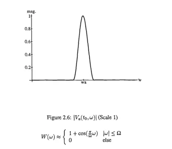
is its FT. The local magnitude spectrum at any time is thus the FT of the analysis window shifted in frequency to wa. The limit on frequency resolution1 0.8 0.6 0.4 0.2
[image:42.595.122.463.150.446.2]wa
Figure 2.6: 1Va (to, w)1 (Scale 1)
w(w) { 1 + cos(Ew) < C2
0 else (2.27)
where Si controls the window bandwidth. The relationship between such a representation and the idealised model is still clear, however. There is still a single stationary band of energy running across time. An appropriate choice of analysis windows and sampling intervals will lead to accurate estimation of the single signal parameter, its frequency. Suppose now that the scale of the representation is changed: the altered window function is more concentrated in time and correspondingly wider in frequency giving increased temporal resolution. The resulting local magnitude spectra of the representation are naturally more dispersed (Figure 2.7) but the form is the same as before: a single peak. Provided that the sampling intervals of this new representation are modified appropriately then the signal frequency may still be obtained without ambiguity. It seems that this signal is accurately represented irrespective of the analysis scale used.
Two Features. Consider now a signal comprising two complex exponentials
= e
jwi t emtCHAPTER 2. REPRESENTATIONS OF AUDIO SIGNALS 33
wa
Figure 2.7: Va (to , w)I (Scale 2)
with frequencies w i and 0)2 . The frequencies and particularly their separation, 0, 2 — wi , could be chosen so that a listener would be able to hear two distinct tones when presented with two sinusoids at these frequencies, for example. In such a case, the desired segmentation of the signal will isolate the two components and estimate their frequencies. Figure 2.8 shows an idealised time-frequency representation of this signal, two distinct bands of energy which is easily related to the listener's perceptions. Forming windowed transforms of this signal at the two scales used before gives the pair of local magnitude spectra in Figures 2.9 and 2.10. Given that the representation is linear these may be obtained from Equation (2.26), giving
Va (t, w) = W(w — 0.4)e_2(w_(1)t m u, _ 0.,2)e—j(w-0,2)t (2.29)
›,.. C..)C
a) a a)
LL LL
i
Time
Figure 2.8: 1Vb(t, (.0)1 (Infinite resolution)
mag.
1- 0.8- 0.6- 0.4-
0.2-w
wl w2
CHAPTER 2. REPRESENTATIONS OF AUDIO SIGNALS 35
Figure 2.10: I Vb(to w) I (Scale 2)
Figure 2.11: I Vc (t, co) I (Infinite resolution)
Scale Restriction 1 The frequency separation of some pair of features will restrict the choice of
analysis scale by defining a frequency resolution below which the probability of successful detection,
with a given window, is unacceptably low.
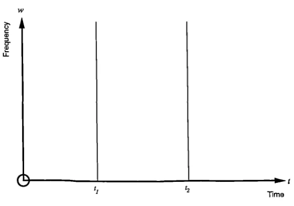
The same effect can be observed in the time domain by considering a signal
7),(0 = 6(t — t i ) O. (t — t2) (2.30)
CHAPTER 2. REPRESENTATIONS OF AUDIO SIGNALS 37
is now finite in time).
Scale Restriction 2 The temporal separation of two features will restrict the choice of analysis
scale by defining a temporal resolution below which the probability of successful detection, with a
given window, is unacceptably low.
Feature Localisation. The signals discussed in the previous discussion were each localised in
only one domain. Clearly such features are idealised and do not occur in natural signals. This work seeks to describe musical signals in terms of a set of features localised, to some degree, in both time and frequency. The localised nature of these features causes them to be 'spread out', making it possible to describe them in terms of their widths (duration and bandwidth) in these domains. A common requirement of feature detection algorithms is that the feature to be detected should fall entirely under at least one of the analysis windows in one or both dimensions. The idealised features examined above are unrealistic: local structure variation is common in natural signals and so the detection algorithms require an analysis window with sufficient width to span the feature. Such local structure decreases the certainty with which the feature's parameters can be determined and gives rise to a further two scale restrictions required to guarantee an appropriate analysis scale.
Scale Restriction 3 For a given detection strategy, the local bandwidth of the target feature restricts
the highest frequency resolution which may be used to detect it reliably.
Scale Restriction 4 For a given detection strategy, the local duration of the target feature restricts
the highest temporal resolution which may be used to detect it reliably.
The General Case Returning now to the more general segmentation problem for the signal shown
in Figure 2.2, it can be seen that all four restrictions can be determined for each feature e.g. Feature 1:
0
<
f2-h
(2.31)I' < t2 — t1 (2.32)
0 > b
1
(2.33)F >
d1
(2.34)Unfortunately the situation is not so simple because the maximum time and frequency resolutions available simultaneously are also bounded by the uncertainty principle (eqn. 2.16) i.e. the four scale restrictions are not independent.
The second pair of restrictions is independent of the signal context, depending only on the extent, in time and frequency, of the feature in question and this can be determined by interactive analysis of various examples of the feature represented over a range of scales. Signal context does, however, determine the first pair of restrictions. Knowledge of the nearest neighbouring features in time and frequency is required before suitable scales can be selected which isolate the feature under investigation. However, the determination of the signal context requires the parameterisation of the neighbouring features which also requires knowledge of their context. This dilemma can be resolved at least partly by careful ordering of the analysis steps, see Chapter 6.
CHAPTER 2. REPRESENTATIONS OF AUDIO SIGNALS 39
one feature from a local data set. Such a scheme for determining the frequencies of two unresolved partials within a duet signal has been described by Nah901 but it is too specialised for a general system. Investigations carried out during the preparation of this work have not revealed any suitable algorithms which reliably implement such multiple-feature detectors for natural signals. The large quantity of local structure variation in such signals (e.g. the beating of coincident partials) introduces a high degree of ambiguity to the data, giving poor results for the simultaneous detection of just two features.
2.3.3 Invariance.
It was mentioned in the introduction that it is desirable for an interactive analysis-synthesis system that the signal representation should be intuitively interpretable by a human observer, additionally this quality simplifies the development of analysis algorithms. Linearity contributes to this, but it is greatly enhanced if the transform shares invariances with the signal features being detected. To illustrate: a note may occur at any point in time; if it is delayed by some amount then none of its perceptual properties (other than onset time) is changed - it is time-shift invariant. It is desirable that the representation of such a note is also unchanged, apart from a time shift. Similarly, if a note's duration is altered or it is transposed in pitch then its representation should reflect this change while remaining unmodified in all other respects. Note that the structure of the wavelet transform gives rise to time-shift invariance but not frequency-shift invariance, so that a note and its transpose would be represented by differing numbers of coefficients. Time and frequency invariances can be satisfied by the use of a regular tessellation of the time-frequency plane i.e. regular sampling intervals of both time and frequency, as is used in the STFT.
2.3.4 Representation Requirements.
3. A choice of resolution at each point on the time-frequency plane.
4. Invariances which correspond to a listener's perceptions.
5. Simple and efficient implementation.
In order to satisfy these demands the approach taken in this work is to use a transform based on the STFT, but which provides multiple representations of the signal, each of which has a different
time-frequency resolution. The transform is referred to as the multiresolution Fourier transform
(mFT) and is a one dimensional form of a scheme recently developed for image analysis [Ca189]. An alternative description of the MFT, including the 2-d form, can be found in that work and [WCPon].
2.3.5 MFT Definition and Properties
The mvr is best introduced by considering again the continuous STFT, but now introducing a scale
parameter a such that
00
f)(t, CO, a)= - Wa(t — r)v(r)e —i"dr (2.35) 03
The scale parameter affects the size of the analysis window which is related to a basic analysis window w(t) via
w(t) =
w(ta)
(2.36)Thus as a decreases, the duration of the analysis window increases, allowing it a greater concen-tration of energy in the frequency domain. As
a —>
0 then the window becomes infinitely long and Equation (2.35) reduces to the continuous Fourier transform.Using this structure the mvr can be considered to be a superset of both the wavelet and STET
(2.41)
CHAPTER 2. REPRESENTATIONS OF AUDIO SIGNALS
41(7), to various transformations. The analysis vectors are simply the appropriate time and frequency shifts of the analysis windows [Dau88a]
= wa (r — t)e
—i
" (2.37)The delaying of such a vector by time St gives
wa (r + St — t)e
—iw(r+6t)
= 7t+a,,,,,a(r)e—jwst
(2.38)a different analysis vector with an appropriate phase shift. Similarly the frequency shift of an analysis vector by S f transforms to another analysis vector.
w,(r —
t)e — (w+ f )1- = 'Y t,((.0 +8 .f),0-(7)
(2.39)These invariances are similar to those of the
sm.
Additionally the MFT'S analysis vectors areinvariant to a dilation by a factor . Using Equation (2.36), such a dilation gives
wa (5,7- — t)e —i" = -yt 6g,scr,,,5,,(7) (2.40)
which corresponds directly to the same operation in the wavelet transform.
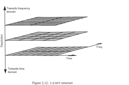
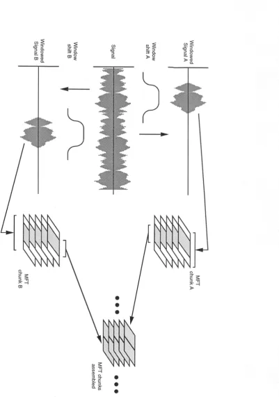
The discrete form of the MFT can now be defined. The overall structure is shown in Figure 2.12. The representation is indexed by three independent parameters: time, frequency and time-frequency resolution. The resolution parameter n selects one of a number of transform levels, each of which is a complete invertible description of the signal, with a structure identical to that of the discrete STET.
Resolution varies uniformly between levels, with the lowest and highest levels being the original signal and its DFT respectively. The level n relates to the scale parameter of the continuous form via
where a is the MFT scale constant. This multiplicity of representations allows the analysis algorithms
Freq.
Time
[image:52.595.111.536.116.397.2]Towards time domain
Figure 2.12: 1-d MET structure
For a finite input signal sequence {x i } : 0 < i < M the transform coefficients are given by M-1
ik( n ) =- (i—ir(n))(n)x le 51(n)kl (2.42)
1=0
where g(n) is the analysis window for level n, F(n) and CI (n) are the time and frequency sampling intervals and all index arithmetic is calculated modulo M. The indices i and k on each level select coefficients from a regular lattice covering the time-frequency plane. There are different numbers of coefficients on each axis for each level, with
0 < i < N(n) (2.43)
and
0 < k < N k (n) (2.44)
For each level to be a complete description of the original sequence, the sampling theorem states that there must be at least the same number of coefficients per level as there were samples in the sequence i.e.
CHAPTER 2. REPRESENTATIONS OF AUDIO SIGNALS
43Choosing the scale constant, p = 2, and constraining the signal sequence length
M
to be a power of two, leads both to efficient computation via the 1-VI and an obvious choice for the number of sample points to satisfy the equality in Equation (2.45)Ni (n) = 2N ' Nk (n) = 2 M =
2
N 0 < n <N
(2.46)and so, for regular sampling, the time and frequency sampling intervals,
F(n) = Nk (n) S2(n) = N2(n) (2.47)
Thus each MET coefficient 2k( n ) represents a rectangular region or 'cell' of the
M
XM
time-frequency plane, of size F(n) x 0(n) and position iF(n), 142(n). These cells are arranged as a uniform time-frequency plane tessellation. Note that each coefficient on level n 1 represents a region of size 21-(n) x 10(n), giving a doubling (a = 2) of frequency resolution and corresponding reduction of temporal resolution; consequently the coefficient pair[k (n), (i_f-i)k(n)] (2.48)
represents the same area of the time-frequency plane as the pair
[(i/2)(2k)(n + 1 ), '(i/2)(2k-E1)(n + 1)] (2.49)
on the level above.
The MET definition leads to the requirements for the analysis windows g(n), clearly they must
be localised in both time and frequency, and ideally should be zero outside a time-frequency region of size F(n) x S2(n).
g(n) = 0 if i <0 i > F(n) (2.50)
(n) = 0 if i < 0 i > S2(n) (2.51)
put in terms of a solution to an eigenvector problem, using linear operator notation
B(S2(n))T(F(n))g(n) = Aog(n) (2.52)
where T(F) is the index limiting operator, an M x M matrix with elements
Oik Ikl <F/2
Tik(F)= 1 0 else The DFT operator F can be similarly defined with elements
1 '21*
Fik = v M
(2.53)
(2.54)
The operator B(S2) in Equation (2.52) is the bandlimiting operator, the frequency domain counterpart of T, which can be defined as
B(52) = F*T(L-2)F (2.55)
where F* is the adjoint of F and is thus the inverse DFT operator. The scalar Ao is the largest
eigenvalue of the combined operator B(F(n))T(S2(n)) and g(n) is the associated eigenvector. In other words an FPSS is a sequence which is unchanged, apart from a linear factor, by the application of time-truncation and bandlimiting operations. The resulting sequences do satisfy the requirements of the MET analysis windows: it can easily be seen from the definition of the combined operator that
these sequences are exactly bandlimited in the interval C2(n), and it has been shown that they have their energy optimally concentrated in the time interval F(n) [WS87a]. The use of bandlimited analysis windows allows efficient computation of the MET using the FFT algorithm.
Extending this linear operator notation, each level of the MET can be defined as
CHAPTER 2. REPRESENTATIONS OF AUDIO SIGNALS 45
F(n) is the nth level MET operator. The parameters of the MFT levels in Equation (2.46) lead to the
observation that the lowest level is simply
F(0) = I (2.57)
the identity operator. At the other extreme, the highest level is the DFT of the original sequence
F(N) = F (2.58)
2.3.6 Oversampled Transform
The above discussion is based on an MET where the number of coefficients on each level is the
min-imum required to satisfy the sampling theorem. However, Equation (2.45) suggests that alternative structures are possible in which a certain degree of oversampling is incorporated. Discussion of the issues behind this type of MET is postponed until the next chapter, where they may be considered
alongside the implementational details of the transform.
2.3.7 Inverse Transform
The overcompleteness of the MET leads to a number of possibilities when defining an inverse transform. Each level of the MET contains enough information to reconstruct the original signal exactly. Thus an inversion operator, F — ' (n), may be defined for each level, such that
x = F 1 (n)k(n) (2.59)
The observation that, since the MET analysis windows are bandlimited to the frequency domain
sampling interval, then the rows of the transform are linearly independent, leads to a definition of the inverse transform's synthesis windows g -1 (n) via the frequency domain relationship [Ca189]
.4,c(n)lign) lki <2(n)/2
within the interval of its support.
An alternative strategy is to devise some sort of inverse operator which uses a set of coefficients selected from more than one level. Clearly there are many possible schemes for the selection process and the choice may be dependent on the application. Some examples have been considered for image reconstruction in [Ca189], but this theme is not pursued further here.
2.3.8 MET Interpretation
Interpretation of the MFT coefficients is analogous to that for the STFT. The analysis window is
localised in both time and frequency, the magnitude of the coefficient thus represents the amount of energy present in a particular region of the time-frequency plane over which the signal is expanded. The uniform time-frequency plane tessellation of each MET level leads directly to the local spectrum and filter bank interpretations suggested for the STFT [Por81].
An MET level can be considered an implementation of a filterbank structure by observing that
each row in Equation (2.42) can be interpreted as a subsampled convolution of an analysis filter g(n) with a frequency shifted version of the signal sequence x i e —jwki , where wk = DSA(n)k. The filters in the bank will have an impulse response similar to the analysis window in the time domain [Por81].
Alternatively, by selecting one column i = io of a level, Equation (2.42) can be written as
= E xi(io)e-MI (2.61)
1=0
which is the DFT of the windowed sequence
CHAPTER 2. REPRESENTATIONS OF AUDIO SIGNALS 47
through the analysis window.
The importance of the use of phase derivatives with respect to both time and frequency in feature identification is discussed in chapters 4, 5 and 6. These partial derivatives must be approximated, in the case of a discrete transform, by the corresponding phase differences which may be obtained via
Pik ( fl ) argPik(n)4(k—i)) (2.63)
vik (n) arg(ik(n)i—i)k) (2.64)
where * indicates the complex conjugate. It can be seen that the desired choices of sampling intervals and analysis window would allow these values to be determined unambiguously from the MFT coefficients. However the choice of window was compromised in that it did not satisfy
Equation (2.51) resulting in a certain amount of leakage between time frames. A means of reducing these errors is discussed in the next chapter.
mFr interpretations involving coefficients from more than one level are fully discussed in Chapter 6, for now it can be seen that the MET definition leads to simple inter-level relationships
such as that between coefficients in equations (2.48) and (2.49). Such simplicity encourages the development of multiresolution models and algorithms using the MET.
2.3.9 S
ummaryMFT Implementation and Initial Results
3.1 Introduction
The previous chapter gave a definition for the MFT and described its properties: the purpose of this chapter is to give a more practical discussion of the mFr and its application to audio analysis. The first section discusses the form of MFT best suited to this application, this is followed by a description
of the actual implementation used in this work. The second half of the chapter presents examples of the MFT applied to some simple signals and discusses their properties.
3.2 Selecting the MFT Parameters
The mFr described in the previous chapter consisted of N transform levels ranging in resolution from the original signal sequence up to its DFr. It has been indicated in several places above that the kinds of signal features of interest to an analysis system are best localised at a scale some way intermediate between these two extremes, suggesting that the extreme levels may be of little use for analysis work. It then follows that this may also be true for other levels close to these extremes, which leads to the conclusion that it may not be necessary, or desirable for storage considerations,
CHAPTER 3. MIT IMPLEMENTATION AND INITIAL RESULTS
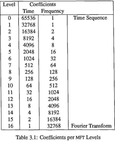
49Level Coefficients Time Frequency
0 65536 1 Time Sequence
1 32768 1
2 16384 2
3 8192 4
4 4096 8
5 2048 16
6 1024 32
7 512 64
8 256 128
9 128 256
10 64 512
11 32 1024
12 16 2048
13 8 4096
14 4 8192
15 2 16384
[image:59.595.166.395.134.417.2]16 1 32768 Fourier Transform
Table 3.1: Coefficients per MFT Levels
to generate all N levels of the MET. Clearly, for a given application, there will be some useful range of levels, nt . .
.nh,
such that0 < ni < nti < N (3.1)
The parameters which serve to characterise each level are:
1. The width of the analysis vector in the frequency domain.
2. The temporal duration of that vector within which its energy is concentrated.
3. The frequency sampling interval, i.e. the distance between the centres of adjacent frequency bins.
4. The temporal sampling interval; this is commonly referred to as the hop-size.
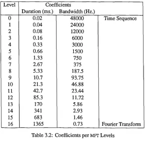
Example values for these parameters are given in tables 3.1 and 3.2 for all the levels of an MET
1 0.04 24000
2 0.08 12000
3 0.16 6000
4 0.33 3000
5 0.66 1500
6 1.33 750
7 2.67 375
8 5.33 187.5
9 10.7 93.75
10 21.3 46.88
11 42.7 23.44
12 85.3 11.72
13 170 5.86
14 341 2.93
15 683 1.46
[image:60.595.135.431.132.421.2]16 1365 0.73 Fourier Transform
Table 3.2: Coefficients per MFT Levels
resolutions desirable for audio analysis; Serra in [Ser89] uses the sTFr with window sizes
as
small as 25 ms. and hop-sizes down to 6 ms, while Watson [Wat86] chooses a hop-size of 10 ms. The frequency resolution required depends heavily on the application; for the purposes of polyphonic music transcription we note that there is 1.64 Hz separating the lowest two notes on a piano and that this represents a fairly extreme case.The mFr considered up to this point has minimum redundancy, each level contains just enough coefficients to be a complete description of the original signal. Section 2.3.6 introduced the idea that alternative structures are possible in which this optimality is relaxed by introducing some degree of oversampling. It has been found, both in this work and in [Ca1891 that these modified forms have a number of advantages over the original definition.
Figure 3.1: Time-Frequency plane FPSS 16 x 32
-32
Time 16
0.75 Amplitude
0.5 0.25
$0'
1,10011L,' •
4.4 S OVIMfz.
V I '
" i I POO'
‘
‘
o
-32
-16
-16
o
32 -48
0.75 Amplitude
0.5 0.25
0 -32
48 32 16
Frequency
-32 Time
16
-16
o
32 -48
CHAPTER 3. MFT IMPLEMENTATION AND INITIAL RESULTS
53Lobe Magnitude (dB)
1 -15.6
2 -20.2
3 -23.0
4 -25.2
Table 3.3: Time Domain Sidelobe Magnitudes for FPSS 16 x 32
Lobe Magnitude (dB)
1 -26.9
2 -32.8
3 -37.1
4 -40.0
Table 3.4: Time Domain Sidelobe Magnitudes for 'relaxed' FPSS 16 x 32
Increasing the truncation width in the frequency domain should result in a vector which is better behaved in both domains. The effect of doing this is shown in Figure 3.2 for an increase by a factor of two. The vector is smoother in the frequency domain and more localised in time, while the sidelobe magnitudes are reduced to the figures shown in Table 3.4. It is related to the original analysis vector by
g'(n) = B(212(n))T(F(n))g(n) (3.2)
and has been termed a 'relaxed' FPSS owing to the relaxation of the frequency domain constraint. In
order to use this modified analysis vector the sampling theorem dictates that, to retain invertibility and the phase relationships in equations (2.64) and (2.64), it is necessary to introduce a corresponding amount of temporal oversampling. The number of coefficients on each level becomes
Art = 2N2 (n) = 21v—n+1 N = N k (n) = 2n N 1(n)nn) = 2M (3.3)
This modified structure has certain other advantages as well as increased temporal localisation. Figure 3.3 shows, for the original scheme, the frequency domain alignment of the shifts of the analysis vector required to generate an MFT level. The corresponding time domain relationship
0.75
0.5
0.25
-96 - -32 0 32 64 96 128
(3.4)
(3.5)
(3.6)
Figure 3.3: Analysis vectors (freq), a = 1
discontinuity. Contrast this with the corresponding relationships for the relaxed version in figures 3.5 and 3.6. Note that there is a loss of frequency resolution, (and corresponding increase in temporal localisation) but that this is accompanied by the avoidance of 'boundary' problems in the frequency domain; there is a smooth transition between adjacent frequency 'bins'.
The resulting tessellations of the time-frequency plane for some MFT level are shown in fig-ures 3.7 and 3.8. Note that in the relaxed version each point on the plane falls under four analysis windows. Each coefficient is now calculated via
M-1
' i.k (n) = z-i g (g(n)-0(n)xie-3171•27., - 14 ,
n
s)k1• 1=00 < i < 2N+1-n 0 k < 2n M = 2N
F(n) =
2
Nu(n)
= 2N—nIn the current MFT implementation, the windows are shifted from the origin in time and frequency
0.75
0.5
0.25
-96 -32 0 32 64 96 128
(
-96 - -32 1
0.75
0.5
0.25
\
CHAPTER 3. MFT IMPLEMENTATION AND INITIAL RESULTS
55Figure 3.4: Analysis vectors (time),
a = 1
Extent of one basis function (a .1)
t
a)
0--96 64 -32 0 32 64 96 128
Figure 3.6: Analysis vectors (time), a = 2
Time