BREVICEPS S'l'OKELL IN
A
S~~LLCANTERBURY LAKE.
A thesis presented for the degree of Doctor of Philosophy in Zoology
in the
University of Canterbury Christchurch, New Zealand,
by
Derek J. §.taples
CONTENTS List of Figures
CHAPTERS
I. INTRODUCTION
II. DESCRIPTION OF STUDY AREA AND GENERAL METHODS OF STUDY
i
v
1
STUDY AREA 6
Local climate 6
Morphometry 7
Water temperature 8
Chemical characteristics 8
Biological characteristics 9
GENERAL METHODS OF STUDY 11
Sampling methods 12
(a) Trap net sampling '12
Selectivity of trap nets 14
(b) Push net sampling 17
Measurement of length, weight and energy content 17
Marking 18
Sex determination 20
Age determination 20
(a) Age determination from scales 20
!
Time an~ periodicity of annulus formation 21 (b) Age determination from length frequency
distribution
(c1 Designation of age
III. LIFE HISTORY, FOOD, FEEDING AND ACTIVITY RHYTHMS
INTRODUCTION 1>1ETHODS
Life history
23
24
26
27
Food habits Feeding rhythms Locomotory activity RESULTS
LIFE HISTORY
Maturation of eggs in the ovary Time and place of spawning
Larval and juvenile fish Size and age at maturity FOOD HABITS
Diel changes in diet
29 30 32 33 33 33 34
35
3637
37
Differences in diet due to sex, season and age 39Differences in diet between sexes Seasonal and age differences in diet FEEDING RHYTHMS
Diel feeding rhythms. Seasonal feeding rhythms . LOCOMOTORY ACTIVITY
39 40 42 42 43 43
Diel activity rhythms 43
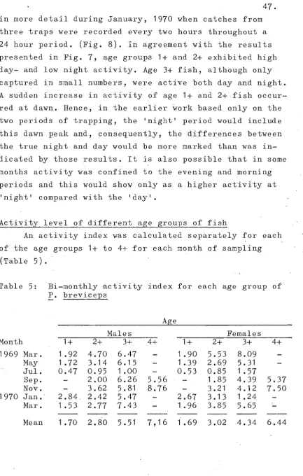
Activity level of different age groups of fish 47
Seasonal activity cycle 48
DISCUSSION
INTRODUCTION METHODS
IV. POPULATION DYNAMICS
opagation of 'error Movements and dispersion
Population estimates and mortality Population fecundity and recruitment Growth in length
RESULTS
MOVEMENTS AND DISPERSION
iii
POPULATION ESTIMATES AND MORTALITY 75
Mark-recapture experiments 75
Uni t volume sampling 78
Population numbers and mortality' 79
POPULATION FECUNDITY AND RECRUITMENT 81
Fecundity 81
Sex and age structure of the breeding
populat-ion 82
Population fecundity 83
Egg survival and recruitment 84
GROWTH IN LENGTH 87
DISCUSSION 89
Movements and dispersion 89
Recruitment 90
Accuracy of population estimates 92
Factors affecting population n.umbers 94
Factors affecting growth in length 98
V.
PRODUCTION, FOOD CONSUMPTIONAND EFFICIENCY OF FOOD UTILIZATION·
INTRODUCTION
METHODS
Production
Production due to growth
Production of sexual products
Food
consumption-Gross efficiency of food conversion
RESULTS
PRODUCT'ION
Length:wei~ht:energy relationships Growth in weight
Production due' to growth
Production of sexual products
Total production
FOOD CONSUMPTION
GROSS EFFICIENCY OF FOOD CONVERSION
DISCUSSION
Production
Factors affecting production Food consumption
Gross efficiency of food utilization
VI. GENERAL DISCUSSION
AND CONCLUSIONS
Suggestions for further workVII. SUMMARY
ACKNOWLEDGMENTS
REFERENCES
APPENDIX
122
125
125
126
127 128
133
135
136
141
LIST OF FIGURES
Following Page
v
CHAPTER II
Fig. 1. The Spectacles Zealand
Lakes, Canterbury, New Fig. 2(a).Rainfall data
(b) • ,vater depth
5 6
6
(c).Monthly water temperature 6
Fig. 3. Map of Spectacles ~akes 7
Fig. 4. Trap net 12
Fig. 5(a).Selectivity curve for trap nets 15 (b).Length frequency distribution corrected
for selectivity bias 15
Fig. 6(a).Scale from Philypnodon breviceps
Fig. Fig. Fig. CHAPTER Fig. Fig. Fig. Fig. Fig. • Fig. Fig. Fig.
showing annuli 21
(b).Scale from
f.
breviceps showing 7. 8. 9. III 1 • 2. 3. 4. 5. 6. 7. 8. 9.annuli and accessory check 21
Time of annulus Length frequency Length frequency age groups
formation
distributions dl.stributions of
22
2-3
23
Size distribution of eggs 33
Annual maturity cycle 34
Size and age at first maturity 36 Diet of Philypnodon breviceps ~n
Large Spectacles 40
Diel feeding periodicity of age 1+ fish 42 Age differences in diel feeding
periodicity 42
Seasonal changes in diel activity rhythms
Diel locomotory activity January, 1970
Seasonal locomotory act
locomotory rhythms, ln ty level
45 45
CHAPTER IV.
Fig. 1. Fig. 2. Fig. 3. Fig. 4.Seasonal dispersal potential Dispersion pattern
Distribution of different age groups Survival curves
Fig. 5. Instantaneous mortality rates Fig. 6(a).FecunditY:length relationship
(b).Fecundity:age relationship Fig. 7.
CHAPTER V.
Fig. 1. Fig. 2. Fig. 3. Fig. 4. Fig. 5. Fig. 6.Nest of Phil~nodon breviceps
Seasonal variation in length:weight relationship
Grow·th in weight
Instantaneous growth rate Monthly biomass
Monthly production
Food ration:weight relationship
68
·73
74
79 80
81 81 85
110
111
112
113
113
1 •
I. INTRODUCTION
The purpose of this thesis was to investigate the relationships between food intake, biomass and production of a population of the upland bully, Philypnodon
Stokell, in a small Canterbury lake.
Early studies of fish populations were confined essentially to descriptive aspects of a species ' biology
(food habits, growth, life history and reproductive
biology). However the inadequacy of this type of information for a complete understanding of the ecology of a fish
population, particularly with respect to management of fish-er s, was soon realised (Ricker, 1946), and in recent
years increasing emphasis has been placed on the more functional aspects of aquatic ecosystems. This approach has been stimulated by the early contributions of such workers as'Thienemann (1926) and Elton (1927), whq first introduced the concepts of trophic levels, ecological niches and ecological pyramids. With the application of the laws of thermodynamics to ecological theory at about the same time (for example, Lotka, 1925), it became poss-ible to consider the dynamic processes associated with the flow of energy through successive levels of a food chain. This trophic-dynamic approach was clearly outlined in the classic paper of Lindemann (1942), which provided a basic model for subsequent research in ecological energetics.
Fish population studies in this field have been
animal or a population can be expressed as:
C
=
P+
R+
F+
Uwhere C is the potential energy of food consumed, P is the energy of production, R is the energy of heat loss and work, F is the energy of unassimilable food passed from the body as faeces, and U is the energy of material lost in urine or through the body surface. Determination of such energy budgets involves a combination of laboratory studies of individual animals and detailed study of the dynamics of natural populations. The present study was confined to field population measurements involving two main categories of the energy hudget: energy intake as food and the production of body tissue and gonad products. With this information i t has been possible to determine
the gross efficiency of ut ization of food for production
(K
1 of Ivlev, 1945, or ecological efficiency of Odum,.
1959) iIi order to describe the amount by which the energy available is reduced at this particular step in the food chain.
In general, studies of production of fish populations have received more attention than consideration of food consumption, but there is still only a limited number of reliable production estimates available. Chapman (1967) has reviewed many of the production studies on freshwater fish and has concluded,tentatively, that production in standing waters in temperate regions ranges from 2 to 15 g/m2/year where a single species predominates. More recently, Elwood and Waters (1969), Walkey and Meakins
(1970), Egglishaw (1970),Libosvarsky and Lusk (1970) and Mathews (1971),have supported Chapman's conclusions.
R.H.K.
Mann (1971), however, recorded a production of"3.
to other aspects of the energy budget, particularly food consumption, (for example, Allen, 1951; Gerking, 1962; Mann K.H., 1965) valuable contributions have been made
to our understanding of the operation of natural eco-systems. It was therefore a primary aim of the present study to relate the production of Philypnodon breviceps to food consumption.
Philypnodon breviceps Stokell, a member of the family Eleotridae, was placed by Stokell (1939) in the Australian genus Philypnodon which is characterised by a scaleless head and ventral surface. Most of the other species of New Zealand Eleotri~ae have been considered to belong to the more fully-scaled genus Gobiomorphus. However, both Cranfield (1962, unpublished) and Woods
(1967, unpublished) considered that all New Zealand
species of this family belong to the genus Gobiomorphus. At present, the upland bully is still generally referred to as Philipnodon brevicepsi although Whitley (1968) in a recent checklist of New Zealand fish referred to the species as Gobiomorphus breviceEs based on a personal communication from ''loods.
The present knowledge of the biology of New Zealand freshwater fish has been reviewed by Hopkins and McDowall (1970). Little information, however, could be provided for ~. breviceps, although the species is common in most rivers and lakes throughout the South Island of New Zealand and the southern region of the North Island. Recent ecological observations of P. have been included by
production dynamics of the population could be con-sidered.
The study of a small fish with a short life
history such as P. breviceps, confined to a small lake system, provided a means of overcoming many of the difficulties inherent in studying natural fish pop-ulations. Many production studies, often because of economic considerations, have been restricted in scope to a consideration of certain age groups of the pop-ulation or have been limited by assumptions concerning the distribution of growth and mortality, especially
for the less-readily captured younger fish. The situation examined in the present study is effectively a simple, small-scale model population with no exploitation by man, few predators, little interspecific competition
and a simple population structure. Under these conditions, the contribution of different age groups to the total
population 'production, the proportion of energy used for reproduction, and the efficiency of food utilization
for production should form an interesting comparison with larger and more complex natural ecosystems.
Because of the small size of the lake, however,
several environmental factors, especially those associated with ~he water-level of the lake, changed abruptly during the study. Consequently, some of the conclusions obtained may be relevant only to the 13-month period of study. On the other hand, the changes that did occur were of suff-icient magnitude to enable detection of associated changes in the fish population, and therefore gave more insight into the factors limiting and regulating production of the study population. ,
5 •
fish uninfluenced by exotic spec s. The results should provide a basis for comparison with populations of bullies in association with salmon (Oncorhynchus tshawytshaGENERAL METHODS
OF
STUDY.
" 1"
I
STUDY AREA
A series of kettle-hole ponds of glacial origin extends across the Lake Coleridge basin, Canterbury, New Zealand (latitude 43018 ' S. longitude 170034 ' E.).
6.
Two of the largest and more permanent ponds occur in close proximity at an altitude of 610 m and are known collectively as the Spectacles Lakes. The general area surrounding the lakes is predominantly tussock grassland interspersed with matagouri scrub (Discaria toumatou) (Fig.1).The lakes are closed, ,with no inlets or outlets, and generally remain separate from each other for most of the year. However, at high water levels, usually in spring, they join across a narrow neck and the fish pop-ulations are then free to interchange.
An investigation into the population ecology of Philypnodori breviceps Stokell was carried out in,the
smaller of the two lakes (Small Spectacles) from February 1969 to March 1970.
Local climate
The climate at this altitude is marked by seasonal extremes, especially in air temperature. Air temperature, recorded on a maximum-minimum thermometer 50cm above
ground level, ranged from a winter minimum of _12.2oC in July 1969 to a summer maximum of 34.4oC in January 1970. A marked diel variation in air temperature was also
recorded, and even in summer night temperatures frequently dropped to 3-4oC.
eight-1
(11)
10
a
8
E
u
... 6
(ij
"l-e ro 4
a::
2
0
3 b
E
2
\
.c
-
e _ _Cl.
...
(J)
...
Cl
'"
0
22
.
, . ... C-',
, , , ,
,
./ t '''
\ ,
18 '-,
' -t
()
'.""'\
,..-,
..
_/'
/
\
0
(J) .... 14
:::J
...
\. f "'-
----
j/ ;'
ro "
....
10 , ,
(J)
Cl.
E
~ 6 , '~/ /
\ ,,'-"--- t
./
2
"""", .. !-t-
/,/,'----OL-~--~---L--_____ ~~~ __ ~· __ ~~~~ __ ~ __ ~ __ - L _ _ - L _ _ ~
F M A M J J A S 0 1\1 D J F M A
1969 1970
7.
month period in the following year 78.5cm were recorded, 50.9cm of which fell during the spring period fromAugust to November.
The prevailing winds are from the north-west, and although shelter for the lakes is afforded by the high rim of the lake basins, considerable mixing of the lake waters occurs. The wind generally increases in frequency and velocity during the spring and autumn
equinoxial periods and is an important aspect of the local climate during these periods.
Morphometr~
Both lakes are situated in steep-sided basins (Fig. 3), with the point of maximum depth at approxi-mately the centre of each lake. The greatest maximum depth recorded for Small Spectacles was 3m and the sur-face area at this time was 9,400m2• The two lakes were joined £or'the first two weeks of the study perio4; the water levels then decreased steadily during the following
seven months, Small Spectacles reaching a depth of only 0.51m and a surface area of 5,790m2 (Fig. 2b). The level then remained constant for the remainder of the study period.
To prevent Small Spectacles from drying up completely after the unusually dry spring period, two pipes of 2.5cm diameter were connected between the lakes from November 1969 to February 1970, bringing a steady flow of water from the higher Large Spectacles to the smaller lake. A fish trap of 1mm2 mesh was used to prevent exchange of
fish between the two lakes during this time.
\
Large
Spectacles
Spectacles
igh water level
m
20 0 20
1 IeewI Iwew!
---lsobat hs
with the larger area exposed to the prevailing north-west wind.
Water temperature
Fig. 2c shows the mean noon water temperature taken at the point of maximum depth over a week period at the beginning of each month. Shore temperatures,
8.
taken at the same time, showed a similar annual cycle, but diel variations were much greater. Similarly, surface water temperatures fluctuated greatly over 24 hours comp-ared with bottom temperatures, and during the day pro-nounced stratification occured, especially in summer. Continous 24-hour temperature recordings on selected days throughout the year demonstrated that the noon tempera-ture approximated the mean daily temperatempera-ture at the lake bottom in winter and autumn but was slightly higher in spring and summer.
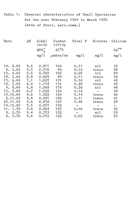
Ice was present on the lake intermittently from early June to August, 1969. Its maximum thickness was 6.Scm but the ice thawed quickly during periods of north-westerly winds. Consequently, little snow accumulated on the ice and light penetration was not severely impaired. Chemical characteristics
[image:22.518.50.472.99.703.2]for the year February 1969 to March 1970
(data of stout, pers.comm.)
Date
pH
Alkal
Conduc
Total
PNitrate Calcium
inity
tivity
HCO;
25
0q
Ca++
mg/l
{'-'mho s / cm
mg/l
mg/l
mg/l
14. 2.69
8.6
0.811
104
0 .. 11
nil
32
9. 3.69
9.3
0.710
99
0.10
trace
28
13. 4.69
9.5
0.707
102
0.07
nil
29
18. 5.69
8.8
0.689
89
0 .. 11
trace
30
1 5. 6.69
7 • 1
1.027
121
0.10
nil
42
12. 7.69
6.4
1 .154
131
0.28
trace
45
9. 8.69
6.8
1.268
139
0.20
nil
48
13. 9.69
6.7
1.028
124
0.14
38
15.10.69
9.6
1 .022
124
0.14
trace
40
2.11 .69
-8.8
0.991
12
9
0.11
trace
41
22.11 .69
9.6
0.858
125
0.40
trace
29
14.12.69
9.5
0.877
130
11. 1.70
9.6
0.804
127
0.04
trace
32
9. 2.70
9.4
0.753
122
nil
29
[image:23.518.32.503.22.696.2]9.
The water of Small Spectacles is relatively soft compared with values given in several other fish pro-duction studies, for example Le Cren(1969), ( [Ca++J ranging from 27 to 48 mg/l) and associated with this is the relatively low conductivity (89 - 139 fmhos/cm). pH was measured during the afternoon on most sampling days and values were high for most of the year (6.7 -9.6), whereas alkalinity values, measured as mg HC0
3-/I, were moderately low. The lake is moderately eutrophic with a high total phosphorus content but, in contrast, nitrate remained low throughout the year. Seasonal changes in pH, alkalinity, conductivity and [Ca++] , were
in-fluenced by three main factors: (1) lowering of the water level, (2) artificial confluence of the two lakes from November 1969 to February 1970, and (3) normal cycles of biological activity_ However, because at least two of these factors were acting concurrently, i t is difficult to assess their relative importance. The effects due to lowering of· the lake and consequent increase of dissolved SOlids, and due to normal seasonal fluctuations, are confounded for the first seven months of the study period. However, from September to March the lake level remained constant and during this period pH increased while both [Ca+1 and [HC0
3-] decreased. The use of CO
2 or HC03- during the day by both rooted plants and algae as soon as they become active in the spring is well documented and normally results in an increased pH and a decreased [Ca (HC0
3)2] through the precipitation of CaC0
3 (Ruttner, 1963).
Biological characteristics
zone around the shoreline. Elodea canadensis and
Myriophyllum propinquum dominated the rooted vegetation, with an occasional patch of Potamogeton cheesmanii
nearer the edge. In summer the growth of Elodea was luxuriant and at this time Elodea was the dominant macrophyte. In winter, however, Elodea died back and Myriophyllum became dominant. Large Spectacles also cont-ained these two weed species although Myriophyllum was more abundant in the larger lake. An extensive bloom of the filamentous green alga ~gnema • occurred in Small Spectacles during the spring but was not present in
Large Spectacles at this time. ,However, an algal bloom occurred later in summer in Large Spectacles.
Zooplankton in both lakes included Polyarthra
and Asplanchna~. (Rotifera) (Livingstone, pers.comm.),
Chydorus sphaericus, Ceriodaphnia dubia, Alona affinis, Alonella macrocopa and Simocephalus vetulus (Cladocera),
Cyclops~. and Boeckella triarticulata (Copepoda). The
weed and mud fauna was dominated by Chironomidae and Oligochaeta. Other insect larvae present included Xanthocnemis zealandica (Odonata), Nymphula nitens
~epidoptera), Paroxyethira ~. (Trichoptera) and
Ceratop-ogonidae (Diptera).
Apart from Philypnodon breviceps,no fish species were present in the lake. Because of the absence even
of eels, which are known to be able to disperse over land, i t is difficult to conceive that bullies were present in the lake through natural causes. Both trout (Salmo trutta) and weed have been released into the lakes by man within the last 30 years but no deliberate attempt to release
11 •
GENERAL METHODS OF STUDY
Monthly production and food consumption were cal-culated for the population of Phil~nodon breviceps in Small Spectacles using a combination of results obtained for fish from both lakes. Population dynamics data were obtained for the bullies in Small Spectacles only, and to avoid interference with these fish, supplementary results on feeding and breeding were obtained from sampl~s taken from LargeSpect~cles.
The sampling program was organised into monthly, bimonthly and seasonal sampling periods.
Monthly: Small Spectacles was sampled for growth estimates (change in mean length of each age group of fish) using trap nets for fish larger than 25mm, and push nets for smaller fish. -Scales were removed f:r:om a stratified subsample of ten males and ten females from each 2mm length-class for age analysis, and all fish
were returned to the population. A separate sample of five-males and five fefive-males in each 5mm length-class was taken from Large Spectacles using push nets. These fish were preserved in 10% formalin immediately after capture and provided material for len~th:weight:energy relation-ships and reproductive maturity analyses.
Bi-monthly: The population in Small Spectacles was estimated using mark-recapture techniques for larger fish and unit-volume sampling for smaller fish. Activity and dispe~sion of the larger fish could also be assessed from the same trap catches.
and food consumption rates of different age groups. '
In addition during the 1969 breeding season fecundity and egg survival were measured in Large Spectacles.
Only the methods common to the complete study will be considered in this section. More detailed methods concerning particular aspects of the study are given in each chapter.
Sampling methods
Two types of nets were used for sampling:
(a) Trap net sampling
Fish were captured using four trap nets modified from a design by Crowe (1950) (Fig. 4). Trap dimensions were: leader 7m x 1m, wings 1 .3m x 1m, pot 1 .2m x 10cm x 10cm, trap opening 1m x 1m, funnel opening 2.5cm in
dia-meter. The trap frame was covered with 1mm2 mesh fabric
netting. All nets were set with the leader perpendicular to the shore and could be operated effectively over the entire lake. During June and July, when ice covered the lakes, the nets were lowered through holes cut in the ice.
Table 2: Month 1969,Feb. Mar. Apr. May Jun. Jul. Aug. . Sep. Oct. Nov. Dec. 1970,Jan. Feb. Mar. 13. Sampling record of E.breviceps for the period February, 1969 to March, 1970 in Spectacles Lakes.
No. of samples 43ge 36gea
4
g 28geam9
g 49geam4
g 37gea4
g 31geam4
g 32geam 3g 27gea 311Trap nets Trap hours 237 203 36 306 110 426 40 307 39 262 31 173 18 190 2,378
No. of fish 13,446 18,738 1 ,046 1·1,653 903 5,032 4,642 13,312 1 ,392 16,382 3,349 16,351 1 ,198 12,279 119,723
Push nets No. of
samples 15gpe 2gp 42gpec 2gp 16gpe 33gpec 12gpe 3gpi 36gpec 2gp 1P 34gpec 2?P 2gp 203
No. of fish 6,276 307 5,092 282 2,869 1 ; 549 1 ,472 431 1 ,470 277 80 2,292 108 80 22,685 g: Samples used for growth estimates (Small Spectacles) e: Samples used for population estimates (Small Spectacles) a: Samples used for activity measurements (Small
Spectacles)
m: Samples used for movement experiments (Small Spectacles) p: Samples preserved for feeding, condition and maturity
analyses (Large Spectacles)
c: Diel samples for food consumption rates (Large Spectacles)
[image:30.518.27.488.82.672.2]Selectivity of trap nets
The significance of trap net selectivity in esti-mating population numbers has been recently considered
(Latta, 1959) but the effect of this bias on growth estimates has been largely ignored. Few accurate
mea-surements of selectivity of traps have been made, although this information is necessary for obtaining unbiased
estimates of both growth and mortality.
The selecti vi ty. of the trap nets in the present study was determined bimonthly from mark-recapture data. The proportion of marked fish captured to those released
(rim)
was calculated separately for each 5mm length-class of bullies (sexes considered separately) on each of the six days of trap sampling. These proportions estimate the probability of capture (p) of thediff-erent size classes
(1).
The relationship betweenprob-o abili ty' of capture and size' of fish was best expressed
after log transformation of both variables, and re-gression lines were fitted to results obtained for each sampling by the method of least squares. The mean and variance of the six successive daily probability values were used for each size class. An analysis of covari-ance comparison between the regression lines indicated that sexes were not being selected differentially at the 5% level of significance (F values for comparison of
slopes ranged from 0.0179 (d.f. ,11) for February 1969·
to 8.4398 (d.f.=1,13) for March 1969; F values for com~
parison of elevations ranged from 0.0055 (d.f.=1,13) to
3.5208 (d .• f. ,12) for May and February 1969,
15. not significant at the 5% level (F value for comparison
of slopes = 1.3631 (d.f.=6,44); F value for comparison
of elevations
=
2.999 (d.f. ,50)).The selectivity of the trap nets could therefore be described adequately by a common regression line based on the whole year's data (Fig.5a). The regression equation was:
log - 7.262
+
3.122 log I (1 )95% confidence limits of the slope were
±
0.440. Anunbiased length frequency distribution was derived from the observed length frequency distribution by correcting the distribution using the above relationship between probability of capture and length of fish, and an
est-imate of the mean probability of capture~ The mean
probability of capturing any fish on a particular day within the sampling period, 'assuming no selectivity effect can be, expressed as:
where
Ii
is the mean probability of capture, fit is themean number of fish caught per day, and
N
is the totalpopulation number. The total population number was
est-imated at bimonthly intervals and these estimates
(i)
are given in a subsequent chapter; hence an estimate of'
Ii
is:and the observed frequency (n.) of successive length
1
.0
ro
.0 0
... 0..
....
Q)
.0 E ::!
Z 0.05
0.04
0.03
0.02
0,01
020
1000
800
I-600
400
200
-0 20
30 40 50
Length (mm)
60 70
30 40 50 60 70
n. I
1
.Q
P
where p. is the observed probability of capture for a
1
given length class, obtained from equation (1).
Selectivity of traps biases the mean of the sample and also affects estimates of population numbers where mark-recapture techniques are being employed. For growth studies unbiased'mean lengths of the samples were est-imated after the described correction technique had been applied (Fig.5b) and for population estimates size
selectivity effects were reduced by stratification of the population into small length classes for analysis.
Patriarche (1968) has suggested that selectivity of trapping devices is caused by differential rates of escape of fish of different sizes from the traps. In the traps used in this study, the mesh size of 1mm2 pre- . vented bullies of all sizes 'from escapingthrough.the walls of the trap, and escape was possible only back through the small funnel opening. In an experiment con-ducted in a pond devoid of bullies in December 1970, 2% of fish escaped during a night setting of 12 hours and 15% during a day setting of 8 hours (sample sizes of 120 and 195 fish, respectively). As there was no significant. difference between the mean lengths of the samples before and after the experiment (t
=
0.06, P> 0.9), i t wasconcluded that fish of all sizes escaped randomly and, therefore, little size selectivity resulted from this cause.
presented in a subsequent chapter, indicates that the behaviour of the fish is the main cause of this size selectivity.
(b) Push net sampling
17 •
Two push nets with rollers, based on a design by strawn (1954), were used to supplement trap net samples. These nets could be used to capture fish of all sizes and also provided fresh material necessary for food
ana-2
lyses. The larger of the two nets had 5mm mesh fabric netting attached to a rectangu~ar frame measuring 120cm x 65cm, while the smaller net was fitted with 1mm2 netting on a frame of 110cm x 50cm.
Both nets could be used effectively under ice after channels had been cut. The number of samples and the
total number of fish collected by push nets each month are shown in Table 2.
A conical tow net of 1mm2 mesh fabric netting, similar to that descrived by Faber (1968), was also used to sample larval fish in the surface waters of Small Spectacles.
Measurement of length, weight and energy content
Length measurements only were taken in the field. Both M.S. 222 and benzocaine were used as anaesthetics but as fish were more tolerant of differing concentrat-ions and temperatures of benzocaine solution, this
material were measured in the laboratory to the nearest 1mg. Food was removed from the alimentary canal before weighing fish,and gonads were removed and weighed
separately to the nearest 0.1mg. Parker (1963) has shown that formalin changes the length and weight of preserved fish. This effect of formalin was determined in the present study from a sample of 40 fish which had been preserved in 10% formalin for one year. Length decreased and weight increased, the preserved values being directly proportional to the fresh values over the entire sire range. These relationships are given by:
Fresh length Fresh weight
1 .025 Preserved length 0.938 Preserved weight. All measurements of preserved fish were corrected by these factors before analysis.
W€t \\reights were subsequently converted to 4ry weights and calorific values. For the purpos€ of this
thesis, energy content was det~rmined for the October sample only, although recently workers have demonstrated marked seasonal cycles of calorific values; for example, values for Cottus gobio L. ranged from 5.5 kcal/g dry weight in spring to a minimum of 4.5 kcal/g dry weight
in winter (Able, pers. comm.). Samples taken of food, fish (without gonads) and gonads were dried at 700C and then reweigh~d to give dry weight values. The fish (wit~ out gonads) were homogenised and the calorific values of subsamples weighing approximately 0.02g were deter-mined using a Parr No. 1411 combustion calorimeter. Gonads and food samples were bombed intact. The total energy content of fish was determined for both sexes on the basis of gonad weight: body weight ratios.
Marking
19. clipping for population estimates and dispersal experi-ments. Different combinations of pelvic, anal, ventral lobe of caudal, and posterior corner of second dorsal fins were used for clipping throughout the study, while recaptured fish were remarked by removal of a coded fin ray from the second dorsal fin. Fin clipping was chosen as a marking method mainly because of the large number of fish which could be processed quickly by one operator. During marking operations a mean of 1,312 fish were
captured, sexed, measured and marked each day.
No mortality could be attributed directly to mark-ing.
A
laboratory experiment was carried out in which 50 fish were marked with all combinations of fin clips and 50 were left unmarked as controls. The mortality of marked and unmarked fish did not differ significantly( 'X-
2 0.36, P 0.6) over the course of the experiment •.An enclosure was also set up in the lake and a similar experiment ·conducted. In this case, over
a
three month period, only one marked and one unmarked fish died. Long term mortality effects were not important, as all mark-recapture experiments extended for a maximum period of 9 days.\'lhen fins were completely removed, as in the case of the pelvic and anal fins, little regeneration occurred during the year. Fish marked in February, 1969 were still recognizable in March, 1970. Partial fin clips, for ex-ample the removal of the ventral lobe of the caudal fin, regenerated within a few months however, and could be used only as temporary marks.
Small fish were marked by immersion ln a Bismarck Brown solution (concentration of 1 :24,000 -water) for four hours. The fish were stained brownish-orange,
Sex determination
Fish larger than 30mm were dimorphic and could be sexed externally all year round from the shape of the genital papilla. The papilla of the female was more obvious, being more bulbous in general shape compared with the triangular papilla of the male. The male papilla was also more heavily pigmented. On subsequent examin-ation of the gonads of a group of fish(50) which had been
sexed by this method, no inaccuracies were recorded. Fish up to 30mm in length were sexed by microscopic exam-ination of the gonads.
Age determination
A method of determining the age of individual
P. brevi~ was fundamental to the study of the product-ion biology of this species. The ability to be able to distinguish age groups of live specimens greatly facili-tates the computation of the production of the total population and the analysis of production processes. Woods (1967, unpublished), in his study of New Zealand Eleotridae, could not find a method for disting-uishing age classes of P. breviceps. However, Hopkins
(1970) isolated age classes of
f.
breviceps using size frequency analysis, and Parrott (1934) showed that the scales of Gobiomorphus (Cuvier and Valenciennes) could be used for ageing. A combination of both these methods was found to be satisfactory for ageingf.
breviceps in Spectacles Lakes.(a) Age determination from scales
21 • the past history of the fish.
Scales of ~. breviceps, taken from the middle region of the side of the body, were preserved dry in small paper booklets and later examined under a micro-scope (x50) using a temporary mount between two glass slides. Fig. 6a illustrates a scale from a 75.4cm bully taken in November 1969. This scale shows the charac-teristic alternate bands of widely-spaced and closely-spaced circuli; the boundary between the closely-closely-spaced and widely-spaced bands defines the annulus, which has been taken as a reference point for age determination. The annulus is also characteriE!ed by cutting-over of circuli at the ventro-Iateral and dorso-Iateral areas of the scale, where the wide circuli appear to cut over the narrow circuli.
Some confusion exists in the literature concerning the nomenclature of these scal~ structures, mainly be-cause of assumptions made concerning their time of for-mation. Following the system of Berg and Grimaldi
(1967), 'circuli' refers to the individual concentric ridges formed on the surface of the scales, and 'bands' refer to groups of similarly-spaced circuli. 'Annuli' are the outer boundaries of the main bands of closely-spaced circuli. lVhere small bands of closely-closely-spaced cir-culi are present, the outer boundaries are considered to be 'accessory checks' as distinct from annuli (Fig. 6b).
Time and periodicity of annulus formation
(
)
(b) 1
(
formula:
R
-r
n r n-1 where G
I is the marginal growth index, R is the total scale radius and r a n d r 1 are the radii of the
ulti-n
n-mate and penultin-mate annuli, respectively. 'Key scales' ( 4 scales away from the caudal fin and one row above the lateral line) were used and all measurements were taken along the maximum radius from the central focus to the tip of the anterior margin, each annulus being
measured to the outer edge of the last circulus of the closely-spaced circuli band. The mean growth index was determined monthly for fish having the same number of annuli, and the weighted population mean was calculated from the proportion of these groups in the population. The monthly marginal growth index of scales from March 1969 to Marcb 1970 1S presented in Fig. 7. As shown by
the sharp decrease in the marginal index, the annulus formed on the scales during August and September. With-in this period the exact time of formation varied between fish, and the midpoint of this period (1st September) was regarded as the mean time of ring formation.
Only one annulus formed during the year of obser-vation. The band of widely-spaced circuli formed during the spring and summer months when scale growth was rapid, and the band of narrowly-spaced circuli formed in autumn. Little growth occurred in winter.
annulus : formation:
I
I
I
I
,
,
1.0 CI,- . •
/
-...-.-.-;
x
~ 0.8
r::
.s:::.
i
0.6e
OJ
~ 0.4
OJ
...
!1l
:2
0.2
i I
I
I
I
I I
I
0~M--~-A--~M~~~J~~IJ~~A~~SS-~CO~~INN~-rD~~19~~~0~FF~
circuli. No other accessory checks could be detected from previous years.
To validate the method of ageing, i t is necessary
23.
to demonstrate that annuli also form in all years of a fish's life as well as during the short term of study. This can be achieved for a fish with a long life history by examining the pattern of annuli-formation of fish of all ages and lengths (Staples, 1971). However, for a fish with a short life history such as P. breviceps, i t was
sufficient to compare scale readings with the length frequency distribution of the fish concerned.
(b) ~determination from length frequenc~ distribution
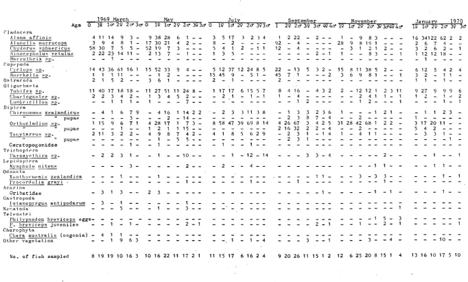
If fish hatch each year during a relatively confined breeding season and grow as a discrete group,* successive year 'classes will be indicated by modes in the length composition of the population. In Fig. 8 the number of
£ish in each 2mm length-class is shown separately for mal~s
and females for each alternate month of study. Three modes are apparent in all samples, indicating at least three age groups. As the whole population was represented in
these samples, the first group must represent fish in their first year of life. By intern~tional convention, these
fish are the age 0+ group, the next group are age 1+, and so on.
The age of a stratified subsample of 10 fish from each 2mm length-class was then determined from scales. The resulting length frequency distribution of each age group for March 1969 is given in Fig. 9 and can be compared with the total length frequency distribution. The modal
Mar.1969 Males Females
No. No.
500 4,938 2,973
'I' 'I'
0
May 1'1'
500 1'1'
2,390
2'1'
0 500
Jul. 1'1' 1,860
0
Sap.
2'1'
500 3,699
L-ID
.0 0
E
::J Nov.
z
1000 2'1'
500 3,830
3'1' 0
Jan. 1'1'
500 3,027
0+ 0
Mar. 1970
500 3,331
0
0 20 80
24. lengths correspond to the first three age groups. Fish known to be age 0+, 1+ and 2+ by length frequency ana-lysis show zero, one and two annuli, respectively. This agreement supports the hypothesis that annuli form re larly each year and that accessory checks were not being included for age determinations, thereby validating the use of scales for age determination. A small group of age 3+ fish were not discernable on the basis of total length, as age 2+ fish overlapped considerably with the age 3+ group. However, as no overlap in length dis
ribution of age groups occurred below 44mm in length, fish below this size limit could be aged simply on a size basis and the use of length frequency analysis appreciably reduced the number of scales which needed to be examined in anyone month.
In practice, smaller fish were aged each month from the length frequency distribution of the month's sample, and larger fish were aged from scales.
(c) Designation of age
estimates, their age designation changing in the middle of the study period. Table 3 gives the year classes involved and their age-group designation during the study.
Table 3: Year classes of
r.
breviceps and their age designation during the study period from February, 1969 to March, 1970.Year class 1969 1968 1967 1966 1965
February 1969-August 1969
0+ 1+
2+ 3+
Age
September 1969-March 1970
0+ 1+
2+ 3+
[image:51.518.33.502.38.698.2]III. LIFE HISTORY; FOOD, FEEDING
INTRODUCTION
Breeding of Philypnodon breviceps Stokell occurs in late spring and summer (Hopkins and McDowall, 1970) and eggs are laid in a ~ingle layer in a primitive nest under stones. The male guards the ne until the eggs hatch, after ,qhich the juvenile fish live in open shallow water and become more cryptic in later life. The seasonal cycle of egg maturation and the size and age at which the bullies first breed, however, have not previously been known,
partly because of a lack of an· adequate method of ageing the species. Recent ecological studies (Cranfield, 1962, unpublished; Woods, 1967, unpublished; Hopkins, 1970) have also given conflicting reports on several aspects of the life history, including the extent of the breeding season, presence of a pelagic larval stage and differences in growth rates between sexes. Other information on the species is widely scattered and is included in a bibli-ography of the indigenous freshwater fish of New Zealand compiled by McDowall (1964). This literature, however, provided little additional information on the species' biology relevant to the present study.
Hopkins (1970) showed that the diet of ~. breviceps in a stream was composed essentially of larval Ephemer-optera and Chironomidae and there appeared to be little competition for food between bullies, trout (Salmo trutta L.) or eels (Anguilla australis schmidti Phillips and
!.
dieffenbachi Gray). There has been little information published.on the feeding of bullies in lakes, and the population in Large Sp~ctacles presented an ~pportunity27. As the trophic relationships within an ecosystem are part of a dynamic, not static, process a descrip-tion of food habits must include diel, seasonal, sexual and age differences in feeding as well as the temporal distribution of feeding and locomotory activity. Many species of fish are known to exhibit periodicity in feeding. However, standard methods for determining feeding rhythms, which simply measure changes in the total weight of stomach contents, indicate only app-roximately the feeding chronology of fish (Darnell and Meierotto,1962). The rate of food passage must be mea-sured as well as stomach weight changes, in order to calculate the dynamics of food intake. As part of a larger experiment designed to measure daily food con-sumption of
f.
breviceps under natural conditions in Spectacles Lakes, food passage rates were measured over four-hourly intervals and, consequently, feeding period-icitiescould be described in terms of food actually ingested in each interval. Diel locomotory activity of fish was also investigated in an attempt to relate loco-motory activity rhythms to feeding periodicities.The aim of this chapter is therefore to (1) describe the basic 1 e history of
f.
breviceps in SpectacleLakes, (2) examine the food and feeding rhythms of the population, and (3) relate feeding rhythms to locomo-tory activity.
METHODS Life history
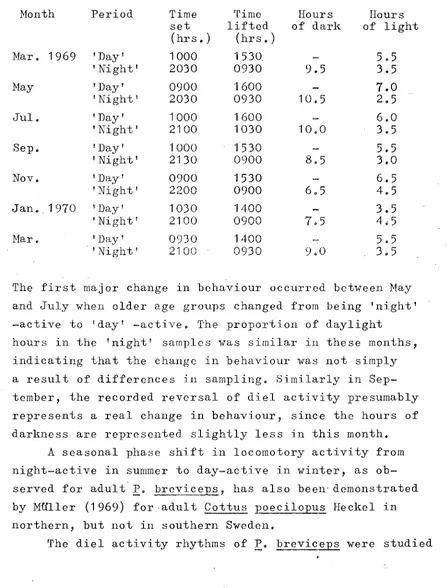
time and duration of the spa,ming season and size and age at first maturity. Fish were captured with a push net; the total length, body weight (minus gonad), gonad weight and the age were recorded for each specimen after preservation in formalin.
The development of gonads and the time of spawning were determined for both sexes and all age groups from changes in the maturity index, which was calculated as the gonad weight (x100) divided by the body weight. Ovaries were removed from the August to January samples and the maximum diameters of all eggs larger than 0.15mm were measured (bymicromeier eyepiece) from a subsample of the combined ovaries of all females larger than 30mm in length. From a monthly average of 340 eggs from 20 females, the size frequency distribution of eggs was
followed throughout the breeding season and the number of egg batches laid by each female derived. Macroscopic
examination of gonads from the October sample (n=97) ena~
hl~ddetermination of the size,and age of fish at first maturity. Gonads were classified as mature or immature on criteria similar to those described by McDowall (1965) for Gobiomorphus huttoni (Ogilby). The presence of secon-dary sexual characters in males (fully developed genital papilla and distinctive colouration) were found to be not necessarily indicative of sexual maturity.
larvae at various stages of development. Continuous temperature recordings were taken throughout the ex-periment.
29.
Other observations on later stages of the life history were made in conjunction with the study of pop-ulation dynamics presented in Chapter 4.
Food habits
Age 1+ fish collected as part of an experiment designed to examine feeding rhythms and daily rations at different times of the year, were also used to in-vestigate diel changes in food. habits from stomach ana-lyses. A total of 425 fish (sample numbers ranged from 9 - 31) collected every 4 hours over three seasonal 24-hour sampling periods were used. Fish were preserved in 10% formal immediately after capture and stomachs were later removed and food items identified and sorted using a dissecting microscope.
After examining diel changes in diet, seasonal changes as well as differences in diet between sex and age groups were examined from material collected at 1400 hours, bimonthly, from Large Spectacles. The fish were aged from scales, the stomachs removed and food items identified and sorted.
To facilitate food analysis, stomach contents of all fish of the same age and sex group were combined before sorting and counting. This procedure greatly reduced the time needed for food analysis, although individual vari-ation feeding could not be measured. However, information on the composition of the diet of separate age and sex
(RxC contingency test, G statistic,; Sokal and Rohlf, 1969). Because of the sensitivity of this test to the contribution of individual variation between fish to the sample differences being tested,analysis of vari-ance techniques were also used for determining differ-ences between sex, season and age. The main effects of these factors were examined by a four-way factorial test without replication. To satisfy the assumptions of normality and homogeneity of variances inherent in this test, the data was transformed by log (X + 1).
Dry weight composition of the major food items was calculated for all monthly samples from the mean dry weight for the different organisms obtained from a
single monthly sample taken in October 1969. Because of the possibility of older fish eating larger indi-viduals of the same food species, dry weight values of food organisms were determined separately for each age group of fish.
Feeding rhythms
Diel feeding patterns were examined for the 1967 year~
31 • gut contents were weighed to the nearest O.1mg in a
moisture-free atmosphere using stable aluminium tainers weighed at a constant temperature. All gut con-tents were expressed as mg per gram of fish.
The amount of food consumed over any four hour per-iod could be determined from the mean weights of gut con-tents of two successive samples
(G
1 and
G
2) and from th0 mean weight of gut contents remaining in the fish kept in the food-free tank over the same period(G
1b). The fish kept in the tank without food gave a measure of the amount
of food lost from the gut (either assimilated by the fish or passed out as faeces) over the four hour period (L):
(1 )
In the lake, however, where the fish could still actively feed, the difference in gut contents of two successive samples. was' a result of the ,relative amounts of food con-sumed (I) and food lost (L) over the period:
(2)
Substituting for L from equation (1), equation (2) be-comes:
Thus, the amount of food consumed over any four hour pe od is equal to the difference, at the end of the per-iod, between the gut contents of the fish feeding in the lake and the fish kept, for the same period in the food-free tank, providing that the rate of food passage through the gut is the same in both groups of fish.
indicated that use of stomach contents alone as first suggested by Bajkov (1935), underestimated the food in-take of bullies, as i t was found that food was capable of passing completely through the stomach in less than four hours. Total gut contents were therefore considered in all analyses.
Locomotory activity
Stratified random trap net sampl~s were taken in Small Spectacles over a 7-day period at the beginning of each alternate month. In the sampling program des-ignedprimarily to estimate population numbers using mark-recapture techniques, most of the trap net sampling was divided into tlvo periods. Nets were set each evening and lifted the following morning; they were then reset in a·new location and lifted again in the afternoon. Although the former period included the dawn and several . hours of daylight, i t lvas considered to be the 'night'
period as compared with the more strictly 'day' period. Since fish swam voluntarily into the trap nets, the· catch over any period reflects the locomotory activity for that period (stott, 1970). The catch per unit time was therefore used to estimate activity, but as changes in density throughout the year would also affect catch rate, an activity index (AI) was calculated as:
n
AI --
t
A
N
where n is the number of fish caught, t is the duration of the trapping period (in hours), A is the surface area
A
33. RESULTS
The section concerning life history includes a des-cription of arbitrarily-defined life history stages in chronological order. The more dynamic aspects of the life history concerning fecundity, growth and mortality are included in Chapter 4.
Examination of food habits and feeding rhythms of P. breviceps follows the life history section, while the last section deals with locomotory activity.
LIFE HISTORY
Maturation of eggs in the ovary
Three categories of eggs could be recognised in the ovaries of mature females just prior to the breeding season. Th~se were (1) small transparent eg~s wit~ dis-tinct granulated nuclei (0.00 to 0.18mm maximum diameter);
(2) creamy white, semi-opaque eggs (0.10 to 0.90mm ); (3) large, yellow, opaque, mature eggs which became more trans~ lucent at maturity (0.80 to 1.60mm ). The monthly size
(])
Ol
(\1
...-c
(])
<..l
I
-(])
a.
10 Aug. 1969
n:351
0
Sep·
10 n=323
0
10 OCt.
n=354
0
Nov.
10 n=375
0
20 Dec.
n:407
O~~~---~ __ ~Cl _ _ _ _ _ _ mdEm __ ~ ______________ ~
40
20
Jan.1970 n=224
. . mature eggs
OL~~~.-~~-,---.r---.---~-.---. ______ . -__ ~ ____ ~
o 0.5 1.0 1.5
For~. breviceps in Spectacles Lakes, the mature eggs of category (3) increased rapidly in diameter from August to October (Fig. 1) and, at a size comparable to eggs collected from nests in the field, decreased in numbers during October, November and December. The eggs of the median group, however, did not increase significantly in mean diameter even during the breeding season. They were
still present in the ovaries at the'beginning of December but were not evident at the beginning of January. As these eggs did not reach a size comparable to those in nests and as spawning activity during December was low (Fig. 2), i t was concluded that these eggs were resorbed rather
than shed during this month. The observation of collapsed eggs of ,this size group in some ovaries supports this con-clusion.
Time and place of spawning
The arinual reproductive cycle as indicated by the maturity index (gonad weight X 100 / body weight) is
..
( \ I1
14
12 Females
10
8
>. ctl x
"0 Q)
... "0
"0 c: 6 Year class
Q) III
E >.
/', I.
o 1968.... ...
• 1967
0 06 -.::
"4-::> III 1966
fJ)
....-... ctl 4
fJ)
~
Q)
z
•
111/
1 1 / - .
2 1 1 1 - 111
-::;::;-...-:::
__
-
IIIII~· III - ; : : ; .
•
0""--0 - 0
0
Males
2
./.---.
.
...-.\
111 111
-0
M A M J J A S 0 N D J F
1969
35. All spawning was confined to the shingly shore region of the lake and eggs were always found on the underside of rocks, usually with a male in attendance. \'/hen equal numbers of three size groups of rocks were provided in the spaw-ning study area, 70% of nests were formed under rocks larger than 15cm in diameter, compared with 28% under rocks 5-15cm in diameter and 2% under rocks less than 5cm in diameter. These larger rocks, however, which appeared to be preferred as nesting sites, were not
numerous in the lake. It is also interesting that two or three nests lvere often present under the same large rock rather than under an adjacent smaller rock. At the peak of the breeding season (November) 61 males occupied nest
sites in the spawning study area of 16.65m2, giving a
2 mean territory size per male of 0.27m •
Larval and juvenile fish
Eggs developed to hatching in a meant1me of 33 days in October (no. of nests =4) at a mean temperature of 14.4°C,whereas only 24 days were required in November
(no. of nests =5) when the mean temperature increased to
o
17.5 C. Hatching of eggs from a single nest extended over a mean period of 10 days in October and 8 days in November, the male remaining with the nest until all the eggs had hatched.
The newly-hatched alevin has a large yolk sac and
1S similar in general morphology to that described by
McDowall (1965) for Gobiomorphus huttoni (Ogilby). The
mean length of an alevin wi thin two days of hatching 'vas
5.05
±
0.04mm (n=53). Pectoral, but not pelvic, fins arepresent on hatchlng and the dorsal fin is broadly
contin-uous ,vi th the caudal _and anal fins. Fin rays are evident
then becomes completely absorbed, pelvic fins develop and the fry begins feeding in the open water of the lake. A gradual movement from a pelagic to a benthic habitat then occurs during the first six months of life.
Cranfield (1962, unpublished), in contrast, con-sidered that young ~. breviceps in Lake Georgina,
Canterbury hatch and commence eding in a habitat sim-ilar to that of adults. However, the open water of the lake was not sampled in his study, and the generali-zation made by Hopkins and McDowall (1970) that ~.
=..;;;;...;....;;;;.,;::...:;.,..t:;.,;:;;.' unlike other species of New Zealand
Eleo-tridae, has no pelagic larval stage needs further exam-ination. Woods (1967, unpublished) considers that all species of New Zealand Eleotridae are active immediately after hatching and maintain themselves near the water surface without resting on the substrate. His laboratory observations are supported by the present study in
Spectacles Lakes where juvenile fish remained pelagic for at least six months.
Size and age at maturity
For each age group, the percent frequency of mature fish in each 5mm length-class in October (just prior to breeding) is shown in Fig. 3. Maturation of both females and males was dependent on the size of fish rather than age, females maturing at a smaller size and less variable age than males. Only 3% of the 1968 year-class females
Females
80
60
40 (j) Age 1 +
III Age 2+
mAge 3+ Q)
20 .. Age 4+
"-:::J
-
t'\lE 0
Q) Cl t'\l
...
100
...
c::
Q)
Males u
"-III
0.. 80
60
40
20
00 10 20 30
37. males had matured by the third year, and 100% breeding for males was observed only in the four-year-old age group.
Males are larger than females at successive ages, and both sexes were found to live to a maximum of 4.5 years. Further aspects of the growth, mortality and sex ratio of the population are considered in greater detail in the following chapter.
FOOD HABITS
A variety of food organisms were eaten by P. breviceps ln Large Spectacles during the. year March 1969 to March 1970. However, within a particular age and sex group at any one time only a few species predominated. Chironomidae
( 3 species), Cladocera (4 species), Oligochaeta (2 species) and Copepoda (2 species) formed the most common constit-uents of the diet. Other food items included Trichoptera larvae (Paroxyethira • ), Odona ta larvae (Xanthoc.nemis z alandica , Lepidoptera larvae (Nymphula nitens and Oribatidae. Cannibalism occurred regularly, the younger members of the population becoming prey to the larger fish; Eggs of P. breviceps were also eaten, particularly by male fish during the breeding season. Bullies in Spectacles Lakes are therefore basically benthic carnivores. Most of the spec ies eaten are characteristica'lly weed and bottom dwelling species (Stout, 1969) and all are common in the weed and bottom mud of Large Spectacles (Livingstone,1970, unpublished).
Diel changes in diet
An average of 2,352 (range 1794-3574) food organisms were identified and counted each season from samples of
age 1+ fish taken every 4 hours throughout a 24-hour period. Each season, and in both sexes, there were significant