Machine Learning based Marks Prediction to Support
Recommendation of Optimum Specialization and Study
Track
Gibrael Abosamra
Computer Information Systems Department, Faculty of Computing and Information Technology, King Abdulaziz University, Jeddah, Kingdom of Saudi
Arabia
Ahmad Faloudah
Computer Information Systems Department, Faculty of Computing and Information Technology, King Abdulaziz University, Jeddah, Kingdom of Saudi
Arabia
ABSTRACT
Due to the spread of educational management information systems (EMIS), it become necessary to add intelligent layers to improve the educational process. One of the important tasks when the student moves from one stage to the other within the educational system of a university is the determination of the appropriate department if the transition is from the first level of a faculty to a certain department or the determination of the specialization track within a certain department in higher levels. These transition moments are crucial because they affect the degree of success of the student in the selected specialization and the quality of the educational process as a whole. In this research, different machine learning (ML) techniques have been tested to predict students' marks based on their marks in the preceded courses to guide them in the selection of the most suitable specialization or track. A variety of ML prediction models have been studied, experimented and evaluated on a propriety dataset, which resulted in the selection of a neural network (NN) architecture that gives an average root mean squared error of 6.26 and a mean absolute error of 5.74 based on a scale of 0 to 100. The accuracy is comparable to the state-of-the-art work and a practical example has been given that proves the ability of the proposed system to recommend certain tracks and/or specializations based on the marks of the already studied courses. Moreover, indirect prediction using cascaded networks has been proven to generate acceptable results that can facilitate building a hierarchy of networks using a short-term dataset to draw a weighted course road map that helps students to select the best path and help institutions to perform early measures to deal with weaknesses and anomalies.
General Terms
Data Mining, Machine Learning
Keywords
Marks prediction, neural network regression, linear regression, logistic regression, support vector machines.
1.
INTRODUCTION
Student’s performance is very important in any university because it affects its academic achievement, which is one of the major criteria in determining its overall quality [1]. Nowadays, there is a huge number of students’ data stored in electronic systems that can be used in the evaluation of students’ performance. The performance of a student depends on many factors through his study. Generally, most of higher learning institutions use the final grades to evaluate students’ performance. Final grades are based on course structure, assessment marks, final exam score and extracurricular activities. This research study benefits from a real prototype
dataset that includes student’s marks to build a ML model that can be used to predict future courses marks of a student based on previous courses marks to guide him in the selection of the majors and/or advanced tracks. The study will go into two different paths. One path is the selection of the best ML model that can be used in the prediction of the new course marks. The second path is the tuning and adaption of the selected ML technique to achieve our goal. The produced ML models can be linked to the EMIS to facilitate and help the student in the selection of his major and/or track based on the approved policy and criteria set by the collage.
The guideline of the research questions proposed in this study are:
Q1: What are the best ML techniques that can be used to predict student marks in a course based on his marks of previous courses?
Q2: What are the best configuration and best parameters to get the best benefits from the selected ML technique?
A predictive modeling is usually built to predict the student performance. In order to build the predictive model, there are two options either dealing with the problem as a classification problem or as a regression one. Most of the done research for predicting the student’s performance is based on classification [1]. There are many algorithms used in the classification task that have been used such as Decision Trees (DT), Random Forests (RF), Support Vector Machines (SVM), Neural Networks (NN), K-Nearest Neighbor (KNN), etc. In this research, the problem will be treated as a regression one to get numeric output that can be used more accurately in the comparison between different tracks or majors.
In addition, many ML techniques will be experimented through two major platforms specifically WEKA and R.
2.
THE RELATED WORK
The usage of EMIS and/or learning management systems (LMS) in education have been increasing in the last few years. This results in many applications that can be categorized into two (not necessarily separable) major fields: learning analytics (LA) and educational data mining (EDM) [2]. The areas of both fields can be summarized into 12 subfields as listed in [2] as follows: Performance Prediction, Attrition Risk Detection, Data Visualization, Intelligent feedback, Course Recommendation, Student skill estimation, Behavior Detection, Grouping & collaboration of students, Social network analysis, developing concept maps, Constructing courseware, Planning and scheduling.Since we are concerned with DM in educational systems, the major topics in which the researchers have concentrated in EDM are listed as follows: Behavior Detection, Skill Estimation, Game-based Learning, Student Modelling, Performance Prediction, Q-Matrix, Adaptive Learning, and Attrition Risk Prediction.Most of the above applications are based on the interaction of the student with the system or in the message boards or discussion forums where the student's activities are monitored, and the student's engagement score is used in either the analysis or prediction applications. As the focus of this research is on performance prediction and course recommendation based on performance prediction, a review of the work related to this subfield will be given in the next section. The given review will be based on two objectives: identification of the variables used in analyzing student’s performance and the existing prediction methods for predicting student’s performance.
2.1
The Important Attributes Used in
Predicting Student’s Performance
The most used attribute that has been used frequently is the cumulative grade point average (CGPA) as per researchers in [1] such as [3, 4, 5, 6, and 7]. Other reported important attributes are combined into one attribute named as internal assessment which includes: assignment marks, quizzes, lab work, class tests and attendance. In other studies, the most often attributes being used are combined into students demographic and external assessments. Students demographic includes gender, age, family background, and disability [5, 8, 9] while external assessments were identified as marks obtained in the final exam for other special subjects [4, 6, 9, 10].
Several researchers have applied the use of Psychometric Factor in predicting the performance of students [11]. A psychometric factor was defined as the student interest, study behavior, engage time, and family support. The last-mentioned attributes are rarely used by researchers because they are mainly qualitative data that can be hardly accurately collected from responders [1]. In this research, the concentration will be only on the obtained marks in the already studied courses since we believe that the marks for most of these studied courses imbed the effect of many attributes from the mentioned ones except the actual activities and engagement of the student when he is enrolled in a new course.
2.2
Techniques Used in Predicting
Student’s Performance
As stated before, in EDM methods, predictive modeling is usually used in predicting the student performance. In order to build the predictive modeling, there are several tasks used, which are classification, regression and clustering.
Classification is viewed as the most popular task in the prediction of the student’s performance. Several algorithms falling under classification have been employed in predicting performances of students. Others have used regression. A review of some of these techniques will be given in the following subsections.
2.2.1
Linear Regression
The problem of regression consists in obtaining a functional model that relates the value of a target response variable y with the values of input variables x1, x2,.., xn (the predictors).
Linear regression is the simplest statistical technique used to find the best-fitting linear curve between the response variable and its predictors for a given n instances dataset represented as:
y = a0 + a1xi1 +···+ ak xik (1)
The solution is reached by finding the parameter vector A (a0,
a1,..,. ak) that minimizes the following distance [12]:
D = (yi− (a0 + a1xi1 + a2xi2 +···+ ak xik ) )2 (2)
2.2.2
Decision Trees (DT) and Model Trees
Most researchers have continued to use DTs which are one of the most widely used techniques of prediction for several reasons among them the fact that they are simple to use and their ability to comprehensively cover both large and small sets of data to forecast values [8, 9]. Romero et al. (2008) attributed the simplicity of DT models to their reasoning procedure and the fact that they can be changed to a set of IF-THEN rules with ease [5]. Several DT algorithms have been used to predict test results to ascertain the likelihood of students to fail based on previous performance data records of students as well as their demographic data [13]. These algorithms include Investigational Device Exemption abbreviated as (IDE), C4.5 and CART (Classification and Regression Trees). Students can be classified based on a number of factors such as their age, level of education, ethnicity and gender as well as their learning environments. This classification can be done through a number of tree classification methods including Quick Unbiased Efficient Statistical Tree (QUEST) and Chi-Squared Automatic Interaction Detector (CHAID) [14].
The counterpart of DTs are Model Trees (MDT), which are used for regression tasks. MDTs are DTs with linear models at the leaf nodes. The most well-known MDT inducer is the M5 algorithm. Since If-Then rules--have the potential to be more compact and therefore more understandable than their tree counterparts, a rule based MDT implementation is currently used in regression tasks where it is called
M5rules[12].
2.2.3
Neural Network (NN)
2.2.4
K-Nearest Neighbor (KNN)
According to [1], KNN was found out to give the best and most accurate performance accuracy. The method also took minimal time to identify different attributes of students’ performance such as a student being an excellent, average or slow learner [6, 16]. This method also gave good accuracy in its estimates on how students advance in their tertiary education [2]. KNN has an implementation version in Weka called IBK (Instance Based Learning with K [17]) that can select the appropriate value of K based on cross-validation and can do distance weighting.
2.2.5
Support Vector Machine (SVM)
SVM technique was also employed to predict students’ performance. According to [18], this method was chosen because it is the best for small sets of data because it has the best generalization ability compared to other techniques. The sequential minimal optimization algorithm (SMO) has been shown to be an effective method for training SVMs on classification tasks defined on sparse data sets. SMO has been generalized so that it can handle regression problems [12]. Its regression version in Weka is called SMOreg.Based on a statistical graph of the different works utilizing the different techniques mentioned above, the used techniques have been ordered in [1] based on their accuracy as follows: ANN (98%), DT by (91%), SVM and KNN having same accuracy (83%).Features used during the prediction process play a role in determining the accuracy of the prediction. Highest prediction accuracy was given by Neutral Network methods. This was attributed to the use of external and internal assessments [4]. The external assessment, defined as the marks obtained in the final examination, is significant in the prediction of student’s performance. Least impact on student’s performance was given by Psychometric factors [11]. Further evaluation of other techniques is mentioned in detail in [1].
3.
DATA UNDERSTANDING AND
VISUALIZATION
3.1
The Study Dataset
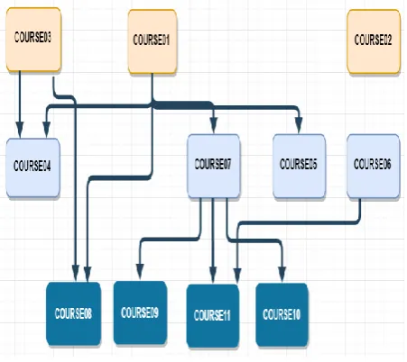
[image:3.595.318.544.72.273.2]A simple dataset, taken from the deanship of information technology at King Abdulaziz University, will be used in this study. The dataset includes marks of eleven courses for 651 students. For the sake of privacy issues, students’ names and courses names are encoded. In addition, the recorded marks are for succeeding students only meaning that all marks are above or equal to 60, which represents the threshold value below which the grade is F (Fail). The course dependency tree for the eleven courses is shown in Figure 1.
Fig. 1: Courses-and-pre-requisite-courses tree.
3.2
Calculating Pair-Wise Correlation
between Different Courses Marks
In this part, the eleven courses in the used dataset that are taught in three consecutive semesters 5, 6 and 7 will be used to discover the linear relationships between these courses using the correlation mechanism. Table 1 displays the correlation coefficients (CRC) between the eleven courses. From Table 1, it appears that some courses are well correlated with others such as COURSE11 with COURSE09 (CRC=0.61) that have a common course in their pre-requisite courses (COURSE07) and may be taught by the same instructor. On the other hand, there are some courses having very low correlation coefficients such as COURSE08 and COURSE09 (CRC=0.12) where there is no common pre-requisite course between them based on the prepre-requisite tree shown in Figure 1.
Table 1: The correlation coefficients between the eleven courses
COU
RS
E0
1
COU
RS
E0
2
COU
RS
E0
3
COU
RS
E0
4
COU
RS
E0
5
COU
RS
E0
6
COU
RS
E0
7
COU
RS
E0
8
COU
RS
E0
9
COU
RS
E1
0
COU
R
S
E1
1
COURS E01
1.00 0.41 0.45 0.49 0.48 0.34 0.37 0.19 0.37 0.31 0.29
COURS E02
0.41 1.00 0.40 0.34 0.38 0.38 0.24 0.21 0.31 0.28 0.32
COURS E03
0.45 0.40 1.00 0.49 0.43 0.48 0.40 0.30 0.42 0.29 0.39
COURS E04
0.49 0.34 0.49 1.00 0.53 0.42 0.40 0.35 0.44 0.47 0.45
COURS E05
0.48 0.38 0.43 0.53 1.00 0.44 0.46 0.43 0.42 0.47 0.38
COURS E06
0.34 0.38 0.48 0.42 0.44 1.00 0.44 0.24 0.41 0.38 0.41
COURS E07
0.37 0.24 0.40 0.40 0.46 0.44 1.00 0.32 0.36 0.48 0.34
COURS E08
0.19 0.21 0.30 0.35 0.43 0.24 0.32 1.00 0.12 0.30 0.24
COURS E09
0.37 0.31 0.42 0.44 0.42 0.41 0.36 0.12 1.00 0.50 0.61
COURS E10
0.31 0.28 0.29 0.47 0.47 0.38 0.48 0.30 0.50 1.00 0.48
COURS E11
3.3
Data Visualization Using Histograms
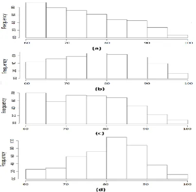
Figure 2 presents four histograms that show the distributions of students among the range of marks (from 60 to 100) for four courses in the current dataset.Fig. 2: Subfigures a, b, c and d represent histograms for the courses COURSE01, COURSE02, COURSE03 and
COURSE04 respectively.
From the shown histograms it appears that, some courses marks are approximately normally (Gaussian) distributed such as COURSE02 while others have non-Gaussian distribution such as COURSE01. In addition, it is noted that some courses have maximum density at the 60 mark because this mark represents the success threshold for a student to pass a course.
4.
DATA NORMALIZATION
Because the range of primary data values varies widely, in some ML algorithms, target functions will not function correctly without normalization. For example, most classifiers calculate the distance between two points according to Euclidean distance. If a feature has a wide range of values, this feature will control the distance. Therefore, all features must be normalized so that each feature contributes proportionally to the final distance.Another reason to apply the feature scaling is that the gradient descent converges faster with the feature scaling more than without it [19]. In the following subsections, the main normalization methods are described briefly.
4.1
Rescaling (Min-Max Normalization)
Also, known as min-max scaling or min-max normalization, it is the simplest method that is based on re-specifying the range of features to rescale the range in [0, 1] or [-1, 1]. The determination of the target range depends on the nature of the data. The general formula is given as follows:x’=(x-min(x))/(max(x)-min(x)) (3)
Where x is the original value and x ' is the normalized value.
4.2
Mean Normalization
In this method, the mean is calculated for an attribute and subtracted from each value and may be scaled by the maximum minus minimum range as follows:
x’=(x-mean(x))/(max(x)-min(x))
(4)
4.3
Standardization
In ML, there are different types of data, for example, audio signals and pixel values for image data, and these data can include multiple dimensions. The standardization of features makes the values for each feature in the data have zero mean (by subtracting the average in the numerator) and dividing by the standard deviation (std) to get a unit variance leading to the following formula:
x’=(x-average(x))/(std(x)) (5)
This method is widely used for normalization in many ML algorithms (e.g., SVMs, logistic regression, and ANN) [20].
In this research, a method appropriate to the type of the academic data will be used based on the selected ML technique. For example, the maximum mark will be assumed as 100 even if the training data does not contain such a mark because predictions will be done based on an unknown test dataset that may contain this full mark within it.
5.
OPEN SOURCE ML AND DM TOOLS
As stated previously, two ML tools (packages) will be used in this research, mainly Weka and R. In the following two sections, a brief description of each will be given.
5.1
Weka
Weka is a Java programming language that deals with the collection of ML algorithms for DM tasks. It is a software application for providing access to the SQL database. The Weka tool is associated with classification, regression, data pre-processing, clustering, visualization, and association rules. It is unable to connect with multi-relational DM, but there is a converter for linking the database tables into one single table [21].
5.2
R-Environment/Programming
Language
R is a programming language and a free software environment for statistical computing and graphics supported by R for statistical computing. R is widely used by statisticians and miners to develop statistical software and data analysis. Surveys, data extraction surveys and studies on scientific research databases show a significant increase in the popularity of R in recent years. Although R has a command line interface, there are several graphical user interfaces such as RStudio which represents an integrated development environment [22].
In the following experiments, Weka will be used first but due to the existence of more ML packages that can be run under R a switch to the R environment will happen where there are multiple-response NN implementations for regression problems that are not available in Weka. [21].
6.
THE ARCHITECTURE OF THE
PROPOSED SYSTEM
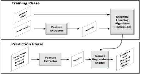
[image:4.595.64.266.125.323.2]Training Phase
Feature Extractor
Machine Learning Algorithm (Regression)
Prediction Phase
Feature Extractor
Trained Regression
Model
Fig. 3: The Architecture of the Proposed System
7.
EXPERIMENTATION AND RESULTS
In this research, experimentation will be based on the dataset described in section 3.1, which can be accessed through the web link [23]. As a general rule in all experiments, an instance is removed if it has any missing value for the specified attributes (courses).
7.1
Normalization
Since the data range is known to start from 0 and end with 100 as this is the traditional numeric range for course marks then a simple normalization method can be used and adjusted to give the best performance of the used ML technique.
In addition, because the dataset includes succeeded students only, hence the minimum value will be 60. In this case, the following formula can be used in normalizing the used dataset:
x’=(x-60)/100
(6)
This will make x’ has a range from 0 to 0.4.7.2
Experiments
In the following subsections, the first four experiments will be done using Weka and the fifth will be done using both R and Weka. All remaining experiments will be done using R only. In all experiments done in Weka, the algorithms will be used based on their default parameters while various parameter values for the ML algorithms used within R will be tried as will be mentioned in the relevant experiments.
7.2.1
Generation of the Learning Curve (RMSE
versus Training Set Size)
The effect of the size (Z) of the training data on the regression accuracy in terms of RMSE and Mean Absolute Error (MAE) will be experimented where Z will be increased by a step of 50 instances while the test sample size will be fixed to 50 instances. A simple linear regression ML algorithm will be used in this experiment. Table 2 presents the change of RMSE and MAE with Z where the dependent variable is the mark of course COURSE04 and the independent variable is the mark of the prerequisite course COURSE01.
Table 2: The Learning table using a simple linear regression ML algorithm.
Z 100 200 300 400 500 600
MAE 7.72 7.37 7.05 6.57 6.6 6 6.68
RMSE 9.34 8.87 8.58 8.15 8.2 3 8.22
[image:5.595.54.282.72.195.2]Figure 4 shows the learning curve as the variation of the MAE and the RMSE w.r.t. Z based on a fixed test set (50 students). From the shown curves, it is concluded that, increasing the training set size increases the system accuracy until reaching to a threshold size of 400 instances after which overfitting occurs.
Fig. 4: The Learning Curve (RMSE and MAE versus Z).
7.2.2
Testing Different ML Algorithms
[image:5.595.321.544.145.254.2]In this experiment, six ML algorithms available in Weka and mentioned in the related work Section will be tested for the same regressionproblem in experiment 7.2.1. Table 3 shows the RMSE and MAE values evaluated for the listed algorithms where 66% of the 651 data instances are used for training and the remaining 34% are used for testing.
Table 3: The output evaluation metrics versus six different ML algorithms in Weka.
ML Model
Linear Regression
M5
Rules
Decision Trees
KNN
(IBK) SVR
(SMOreg) MLP
MAE 6.19 6.19 6.25 6.39 6.14 6.33
RMSE 7.69 7.69 7.67 7.84 7.66 7.75
From Table 3, it appears that the best ML learning model is SVR based on RMSE and MAE. In addition, there are other algorithms, which gave nearly the same results such as the linear regression and M5Rules. Since only one input variable is used in this experiment, the selection of the best ML algorithm shouldn’t be done until doing more experiments that will be presented in the following subsections.
7.2.3
Testing the effect of the number of features
(input courses marks) on the accuracy of the ML
algorithm
In this experiment, experiment 7.2.2 will be repeated for the same output course mark (COURSE04) but with more input courses (3 courses: COURSE01, COURSE02, and OURSE03). Table 4 lists the evaluated metrics versus different ML algorithms in Weka for one dependent output (course) and 3 independent variables (courses).
Table 4: Evaluation metrics versus ML algorithms in case of 3 input variables.
Linear
Regression M5
Rules
Decision Trees
KNN
(IBK) SVR (SMOreg) MLP
MAE 5.09 5.09 6.58 7.87 5.15 5.08
[image:5.595.315.542.383.453.2]From Table 4, it is clear that the minimum RMSE is produced when using the MLP giving 6.55. By comparing this result with that in the previous experiment (7.75), it will be concluded that increasing the number of features to 3 courses reduces the MLP RMSE value by a percentage of 15%.
Figure 5 displays the RMSE and MAE versus the used algorithms in the current experiment.
Fig. 5: RMSE and MAE versus the used ML algorithms
7.2.4
Comparing the Results for Different Output
Courses Based on the Same Input Courses Using
the MLP.
[image:6.595.315.542.86.157.2]In this experiment, the MLP will be used to detect the marks of the four courses (COURSE04, COURSE05, COURSE06 and COURSE07) based on the same input courses used in the previous experiment (COURSE01, COURSE02, and COURSE03). The results are shown in Table 5.
Table 5: MAE and RMSE for 4 output courses based on 3 input courses.
Output Course
s
COURSE0 4
COURSE0 5
COURSE0 6
COURSE0 7
MAE 5.08 7.52 7.24 6.03
RMSE 6.55 9.67 9.11 7.73
From Table 5, it is obvious that COURSE04 has the best results because its marks are more correlated (CRC is 0.49 as shown in Table 1) with two of the input courses (COURSE01 and COURSE03) that are pre-requisite courses for it. The second-best results are for COURSE07 which has only one of the inputs as prerequisite (COURSE01) although its linear correlation coefficient is low as shown in Table 1(CRC=0.37) which means that there are other non-linear correlation relationships that the MLP has used in predicting the output.
7.2.5
Comparing the NN implemented in R with
the MLP implemented in Weka
In this experiment, the results of the MLP in Weka will be compared with the results of the NN in R based on the same input and output courses of the previous experiment. While the MLP in Weka has multi-input and single output architecture, the NN implemented in R has multi-input and multi-output which is configured in this experiment with one hidden layer that has 12 neurons. Tables 6 and 7 show the results in case of Weka and R respectively.
Table 6: Results when using MLP in Weka.
MLP
(Weka)
COURS E04
COURS E05
COURS E06
COURS
E07 Average
MAE 5.08 7.52 7.24 6.03 6.47
RMSE 6.55 9.67 9.11 7.73 8.26
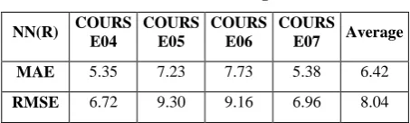
[image:6.595.56.282.151.323.2]In case of the NN in R, the following parameters are chosen: Activation function: logistic, error function: sum of squared errors, and resilient backpropagation algorithm [24].
Table 7: Results when using NN in R.
NN(R) COURS E04
COURS E05
COURS E06
COURS
E07 Average
MAE 5.35 7.23 7.73 5.38 6.42
RMSE 6.72 9.30 9.16 6.96 8.04
By comparing the two tables, it will be concluded that the results of both implementations are alternating; meaning that two courses have better results in Weka (COURSE04 and COURSE06) and two courses have better results in R (COURSE05 and COURSE07) but the average result of the four courses in R is better than that in Weka. Hence it can be concluded that modelling the relation between the three input courses and the four output courses using a single NN in R has the benefits of more generalizations, which cannot be achieved with the current Weka implementation that supports single output only.
7.2.6
Comparing Results Based on Different
Previous Terms
In this experiment, the predictions done for a specific term will be based on one or two previous terms. Specifically, marks for courses taught in term 7 will be predicted based on marks in term 5 and/or term 6. The NN will have one hidden layer with 12 neurons in the three cases below to do fair comparisons although different configurations may give better accuracies for each case. Table 8 shows the results of the prediction of marks of courses in term 7 based on courses taught in term 5. Training is done on 308 students and testing is done on 125 different students. Table 9 shows the results of the prediction of marks of the same courses in term 7 based on courses taught in term 6.
Table 8: Prediction of marks in Term 7 (COURSE08, COURSE09, COURSE10 and COURSE11) based on
marks in Term 5 (COURSE01, COURSE02, and COURSE03).
NN(R) COURS E08
COURS E09
COURS E10
COURS
E11 Average
MAE 7.08 6.34 5.96 7.49 6.72
[image:6.595.315.542.213.281.2] [image:6.595.56.279.464.538.2]Table 9: Prediction of the marks of the courses in Term 7 based on the marks of the courses in Term 6 (COURSE04,
COURSE05, COURSE06 and COURSE07)
NN(R) COURS E08 COURS E09 COURS E10 COURS
E11 Average
MAE 6.67 5.31 5.53 7.02 6.13
RMSE 8.33 6.45 7.06 8.31 7.58
Table 10 shows the results of the prediction of marks of the same courses in term 7 based on the courses taught in terms 5 and 6.
Table 10: Prediction of the marks of the courses in Term 7 based on the marks of the courses taught in Terms 5 and
6.
NN(R) COURS E08 COURS E09 COURS E10 COURS
E11 Average
MAE 6.5 5.34 5.33 6.51 5.92
RMSE 8.38 6.43 6.92 7.82 7.43
From Tables 8 and 9, it is concluded that the prediction errors are reduced if prediction is done based on the nearest term marks. In addition, from Tables 8, 9 and 10, it is noted that predictions are enhanced if more features (course marks) are used by including two term marks instead of one term as input to the NN. This can be justified by the fact that knowledge and skills needed for a certain course may depend on the knowledge and skills learned in multiple courses taught in different terms or levels.
7.2.7
Testing Other Normalization Methods
[image:7.595.314.543.71.140.2]In the previous experiment a simple and effective normalization method has been used, but to be sure, all methods mentioned in Section 4 will be tried with fixed statistical parameters to allow single instance prediction as follows: min(x):60, max(x):100, mean(x):80 and std(x):10. In addition, two activation functions, specifically the hyperbolic tangent (tanh) and the logistic sigmoid will be tried because the normalization methods and the activation functions have combined effects on the accuracy of the NN model. The results for the average MAE and RMSE after trying all the combinations available in the NN implementation in R including the final output activation (linear or non-linear) are shown in Table 11 for the same experiment presented in Table 10 using a single hidden layer with 20 neurons.
Table 11: Predicting marks for term 7 based on marks in terms 5 and 6 for different combinations of normalization
methods and activation functions.
O u tp u t La y er Ac tiv a tio n H id d en La y er Ac tiv a tio n Metr ics Re sc a li n g (3 ) Mea n No rm a li za tio n (4 ) S ta n d a rd iza ti o n (5 ) O UR S (6 ) Non-Linear
logistic MAE
6.1 6.14 6.46 6.09
RMSE 7.59 7.63 8.2 7.57
tanh
MAE 6.56 6.06 8.23 6.21
RMSE 8.88 7.7 10.52 7.74
Linear
logistic
MAE 6.28 6.69 7.75 6.38
RMSE 7.84 8.46 9.73 7.85
tanh MAE
6.31 6.41 7.99 6.04
RMSE 7.97 8.04 10.32 7.64
From Table 11, it is apparent that the proposed normalization method defined by (6) is the best regarding the minimum RMSE (7.57) when selecting the logistic function for the hidden layer and non-linear activation for the output layer. On the other hand, (6) is the best if we regard the minimum MAE (6.04) when using the tanh function for the hidden layer activation and linear activation for the output layer.
7.2.8
Testing the Effect of Adding Information
Other Than Mark Values
In this experiment a new attribute related to the campus will be added as an extra input which designates one of three campuses; Male, Female (A), and Female (B). Each campus will be represented with a numeric value as follows: Male (:1), Female (A: 2), Female (B: 3). Using trial and error, a good normalization method for the campus attribute is found by dividing it by 8.
[image:7.595.55.280.108.172.2]After training and testing, better results are produced as shown in Table12, for the same input and output courses shown in Table 10 when using logistic activation for the hidden layer (with 14 neurons) and non-linear activation for the output layer.
Table 12: Predicting marks for term 7 based on marks in terms 5 and 6 after using the campus attribute.
NN(R) COURS E08 COURS E09 COURS E10 COURS
E11 Average
MAE 6.28 5.03 5.14 6.49 5.73
RMSE 8.07 6.15 6.49 7.66 7.14
7.2.9
Testing Other NN Implementations with
More Hidden Layers
In this experiment, deep learning with R will be tested based on the same data used in the previous experiment. While in previous experiments, a single hidden layer was used, in this experiment the DeepNet package [25] with two hidden layers having 20 and 10 neurons respectively will be used. The results for both implementations are shown in Table 13.
Table 13: Output results based on two hidden layers using DeepNet and NN.
Metr
ics
CO
UR
S
E
0
8
CO
UR
S
E
0
9
CO
UR
S
E
1
0
CO
UR
S
E
1
1
Av
er
a
g
e
NN MAE 6.5 5.01 5.24 6.54 5.82
RMSE 8.21 6.16 7 7.8 7.33
DeepNet MAE 6.64 4.73 5.24 5.17 5.79
RMSE 8.57 5.94 6.61 7.8 7.16
Figure 6 displays the change of RMSE and MAE with the value of the momentum for the same problem with a learning rate of 0.6, tanh activation function for the hidden layers and linear activation for the output layer.
Fig. 7: RMSE and MAE versus Momentum in DeepNet for the same problem in Table 13.
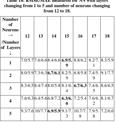
[image:8.595.314.544.194.320.2]By using a momentum of 0.8 and changing the number of layers from 1 to 5 and the number of neurons of all layers from 8 to 30, less values for the RMSE and the MAE can be found. Table 14 displays part of the results of this search that contains the minimum values of RMSE/MAE (with bold face).
Table 14: RMSE/MAE measured for NN with layers changing from 1 to 5 and number of neurons changing
from 12 to 18.
Number of Neurons
→ /Number of Layers
↓
12 13 14 15 16 17 18
1 7.0/5.7 7.6/6.6 8.4/6.6 6.9/5. 9
8.8/6.2 8.2/7. 1
8.3/5.9
2 8.0/5.9 7.3/6.3 6.7/6.1 8.2/5.
9
6.8/5.8 7.4/5. 9
9.1/7.7
3 8.3/6.5 8.4/7.4 8.0/5.8 8.1/6.
4
6.7/6.3 7.4/6. 5
8.6/6.5
4 7.6/6.3 6.4/5.6 6.8/7.2 6.3/6. 0
7.2/5.4 7.6/6. 2
8.1/6.7
5 9.3/7.6 10/7.7 6.9/5.9 9.1/7.
3
10.7/7. 8
7.9/5. 8
7.2/6.6
From Table 14, it appears that increasing the number of layers does not give significant enhancements in case of having layers of the same number of neurons. As a final test, the previous search for minimum RMSE will be repeated but with varying the number of neurons for different layers and only the optimum number of neurons will be reported for each layer (from 1 to 4 only) for the two implementations (DeepNet/NN) as shown in Table 15.
Table 15: The Optimum number of neurons in each layer of an N-layer NN (using DeepNet/NN) to get minimum
RMSE.
Optimum Number of
Neurons Metrics
Number of layers
Layer 1
Layer 2
Layer 3
Layer
4 RMSE MAE
1 15/8 6.9/7.3 5.7/5.8
2 22 /29 13/23 6.4/7.3 5.6/5.8
3 29/27 21/27 18/14 6.2/7.2 5.74/5.7
4 17/29 17/23 16/23 10/15 6.2/7.2 5.9/5.7
From Table 15, it is observed that, using three layers with DeepNet reduces the RMSE by about 0.7 compared to one layer. Increasing the number of layers than three does not give significant enhancements in the RMSE value but increases the corresponding MAE value. This means that more complex mapping (deeper network) will not give more significant enhancements because the relationship between the response variables and the input variables is partially represented by a linear relationship and a smaller fraction is due to some non-linear correlation that is partially related to the male/female campuses where differences may be due to differences in the instructors and/or the students. The differences in the instructors surely represent a major factor in the non-linear relationship portion because each instructor has his own way of teaching and evaluation as it concluded from the marks histograms shown in Figure 2. Comparing with a recent study [26] that used Restricted Boltzmann Machines (RBM), which gave the best result in this study, it is found that the minimum RMSE reported on a 0.0 to 4.0 scale was 0.3, which will be 7.5 when converted into 0.0 to 100.0 scale. This value (7.5) is greater than the overall RMSE value (6.2: using three hidden layers with DeepNet) shown in Table 15. Based on this study and on the performed experiments it can be concluded that using ANN in mark prediction is beneficial in recommender systems as will be emphasized by the final experiment.
7.2.10
Testing Indirect Prediction Using
Cascaded Networks
In this experiment, two different NN networks will be trained. The first neural network NN1 will be trained to predict the marks of courses in term (n) based on the marks of courses in term (n-1) and the second neural network NN2 will be trained to predict the marks of courses in term (n+1) based on the marks of courses in term (n). To predict the marks of courses in term (n+1) based on the marks of courses in term (n-1) the marks of term (n-1) will be fed into NN1 and the outputs of NN1 will be fed as inputs to NN2 and hence the predicted marks of courses in term (n+1) will be produced as the output of NN2 as shown in Figure 6.
4.00 6.00 8.00 10.00
0.00 0.10 0.20 0.30 0.40 0.50 0.60 0.70 0.80 0.90 1.00
Momentum
[image:8.595.54.283.285.416.2] [image:8.595.54.283.519.761.2]Fig. 7: Prediction of the courses marks at term N+1 based on the courses marks at term N-1 using two cascaded
networks.
[image:9.595.315.542.97.160.2]To test the proposed configuration, the predicted marks for courses in term 6 based on marks of courses in term 5 will be used to predict marks of courses in term 7 using NN1 followed by NN2. The results are shown in Table 16.
Table 16: Predicting marks for term 7 based on marks predicted for term 6 depending on actual marks in term 5.
NN(R) COURS0 8
COURS0 9
COURS1 0
COURS1
1 Average
MAE 6.62 4.49 5.55 6.54 5.80
RMSE 8.32 6.12 7.15 8.03 7.46
Comparing the results of Table 16 with that in Table 13, small differences are observed in the recorded errors although the prediction here is indirect using two normal NNs each having a single hidden layer with 14 neurons. Hence, by using indirect prediction, the required NN models needed for prediction and the size of the required dataset can be minimized where records for two years or less will be enough to build all needed models. Based on this experiment we can conclude that, indirect prediction using cascaded networks can generate acceptable results that can facilitate building a hierarchy of networks using a short-term dataset to draw a weighted course road map that helps students to select the best path and help the institutions to perform early measures to deal with weaknesses and anomalies.
7.2.11
Recommendation of Tracks and/or
Specializations Based on Studied Courses
The goal of this experiment, is the prediction of the marks of two different specializations, specifically Information Technology (IT) and Software Design (SD), where two suitable courses are selected for each specialization (COURSE04 and COURSE08 for IT and COURSE07 and COURSE10 for SD). A NN model with 2 hidden layers having 20 and 10 neurons respectively will be used with four inputs and four outputs. The predicted marks will be used to select the specialization for a certain student based on the average of the two courses in each path. The network model is built based on three primitive courses taught in the preceding term (mainly COURSE01, COURSE02, and COURSE03) and including the campus attribute as a fourth input. The results of this testing are shown in Table17.
Table 17: Prediction of 4 courses marks based on the marks of 3 previous courses.
NN(R) COURS0 4
COURS0 8
COURS0 7
COURS1
0 Average
MAE 4.95 6.92 5.32 5.86 5.76
RMSE 6.17 8.59 6.99 7.61 7.39
Table 18 presents the predicted marks for some of the students who are advised to take the IT path based on the calculated average for each path while Table 19 presents the predicted marks for students who are advised to take the SD path based on the calculated average for each path.
[image:9.595.315.540.318.489.2]Although the differences between the averages of the two paths are not so large, a ML based recommendation method is introduced for the student or the advisor to guide the student to the better path. Hence, the experimented model can be implemented and added as an important tool in the academic advising system.
Table 18: Sample of students who are guided to IT path.
Std
NO COURSE04 COURSE08 COURSE07 COURSE10 IT
path SD
path
363 97.91 90.29 92.17 92.92 94.10 92.55
339 96.92 89.26 91.07 92.04 93.09 91.56
377 92.19 88.321 88.21 90.24 90.26 89.23
423 92.946 87.46 88.49 89.97 90.20 89.23
367 91.66 88.74 88.16 90.33 90.20 89.25
416 93.09 87.64 88.73 90.12 90.37 89.43
428 93.59 89.63 89.98 91.38 91.61 90.68
420 91.53 87.58 87.62 89.65 89.55 88.63
Table 19: Sample of students who are guided to SD path.
Std
NO COURSE04 COURSE08 COURSE07 COURSE10 IT
path SD
path
334 73.21 76.09 76.34 79.364 74.65 77.85
376 74.48 77.61 78.22 80.26 76.05 79.24
323 76.25 78.92 80.11 81.40 77.59 80.75
353 74.26 77.04 77.36 80.01 75.65 78.68
320 74.58 77.92 78.14 80.35 76.25 79.25
[image:9.595.56.282.354.415.2]44.8 are advised to take the SD path which can be considered a balanced distribution. The selection between using standardization or not can be optional or imposed based on the policy of the institution. It can be also offered to the students to select either the path with maximum expected marks (or CGPA) or the path that gives relative Excellency (or better skills) within the selected specialization. This situation is like selecting a job that gives the maximum salary or the one that gives the maximum experience.
8.
CONCLUSION AND FUTURE WORK
In this research, many ML techniques have been tried to predict student’s marks. Although a small accuracy differences were noted between most of them, ANN was proven to give the best results because it can model both linear and non-linear correlation between independent and response variables. In addition, multi response output of available NN implementations make it easier to predict the marks of many courses at once which supports the targeted goal of giving an expected course marks road map for the student to select between the different tracks and/or specializations. Due to the continuous change of the educational environment with time, retraining of the used models is necessary every fixed period (may be one semester or two). Not only students will benefit from the prediction models but also the educational institutions can use them to discover anomalies and weaknesses of the courses, the prerequisite courses and the teaching style of the responsible instructors. Moreover, predictions of the higher-level courses can be done with a reasonable accuracy that can allow the educational institutions to perform early measures to treat weaknesses and guide students to their best tracks. A very impressive conclusion is that a huge multi NN can be built to predict courses marks at any level in a faculty or a university where each network is trained to predict the marks of level n based on level n-1 and when there are missing values for courses marks in a certain level, the missing marks can be deduced using lower level networks. Each network can be 2 to 3 layers and the inputs may be based on one or two previous levels. Experimentation of such a huge system needs a big data set and is left for future work.
9.
ACKNOWLEDGMENTS
Our thanks are to the Deanship of Information Technology at King Abdulaziz University, which supplied us with the elementary dataset used in this research. Also, the authors wish to thank all the FCIT members especially the Dean and the Head of the CIS department for the facilities provided to complete this research
.
10.
REFERENCES
[1] A Shahiri, W. H. 2015. A Review on Predicting Student’s Performance using Data Mining Techniques. Procedia Computer Science, Vol 72, pp.414-422.
[2] Sin, K., and Muthu, L. 2015. Application of big data in education data mining and learning analytics – a literature review. ICTACT journal on soft computing. Vol 5-No.4.
[3] Romero,C., Ventura, S., Espejo, P. G., and Hervas, C. 2008. Data Mining Algorithms to Classify Students. In Educational Data Mining 2008.
[4] Angeline, D. 2013. Association Rule Generation for Student Performance Analysis using Apriori Algorithm. The SIJ Transactions on Computer Science Engineering & its Applications (CSEA). Vol.1-No.1., pp.12-16.
[5] Naren J. 2014. Application of Data Mining in Educational Database for Predicting Behavioural Patterns of the Students. International Journal of Computer Science and Information Technologies, Vol.5-No.3, pp. 4649-4652.
[6] Mayilvaganan, M., and Kalpanadevi, D. 2014. Comparison of classification techniques for predicting the performance of students’ academic environment. Communication and Network Technologies (ICCNT), (pp. 113–118). Coimbatore: IEEE.
[7] Parack S., Zahid, Z., and Merchant, F. 2012. Application of data mining in educational databases for predicting academic trends and patterns. Technology Enhanced Education (ICTEE), (pp. 1–4). India: IEEE International Conference.
[8] Osmanbegovic, E., and Suljic, M. 2012. Data mining approach for predicting student performance. Economic Review - Journal of Economics and Business,Vol.10-No.1 pp.3-12.
[9] Natek, S., and Zwilling, M. 2014. Student data mining solution–knowledge management system related to higher education institutions. Expert Systems with Applications, Vol.41-No.14, pp.6400–6407.
[10] Arsad, P., Buniyamin, N., and Manan, J. 2013. A neural network students' performance prediction model (NNSPPM). Smart Instrumentation, Measurement and Applications (ICSIMA) (pp. 1–5). IEEE International Conference.
[11] Gray, G., McGuinness, C., Owende, P. 2014. An application of classification models to predict learner progression in tertiary education. International Advance Computing Conference (IACC), (pp. 549–554). Dublin, IEEE.
[12] Kotsiantis, S., and Pintelas, P. E. 2004. Comparing Regression Algorithms for Predicting Students’ Marks in Hellenic Open University. Accessed through http://www.etpe.gr/custom/pdf/etpe55.pdf
[13] Yadav, S., and Pal, S. 2012. Data Mining: A Prediction for Performance Improvement of Engineering Students using Classification. World of Computer Science and Information Technology Journal (WCSIT), Vol.51.
[14] Kovacic, Z. 2010. Early Prediction of Student Success: Mining Students’ Enrolment Data. Proceedings of Informing Science & IT Education Conference (InSITE) (p. 648). Informing Science Institute.
[15] Tu, J. V. 1996. Advantages and disadvantages of using artificial neural networks versus logistic regression for predicting medical outcomes. Journal of clinical epidemiology,Vol. 49-No.11,pp. 1225-1231.
[16] Minaei-Bidgoli, B., Kashy, D. A., Kortemeyer, G., and Punch, W. F. 2003. Predicting student performance: An application of data mining methods with the educational web-based system. Frontiers in Education, 2003. FIE 2003 33rd Annual,Vol.1, pp. T2A-13. 1, USA: IEEE.
[17] Aha, D. W., Kibler, D., and Albert, M. K. 1991. Instance-based learning algorithms. Machine learning, Vol.6-No.1, pp. 37-66.
Tutoring Systems (pp. 525-534). Springer, Berlin, Heidelberg.
[19]Wikipedia contributors. (2018, November 25). Feature scaling. In Wikipedia, the Free Encyclopedia. Retrieved
12:10, March 3, 2019,
https://en.wikipedia.org/w/index.php?title=Feature_scali ng&oldid=870599160
[20]Grus, Joel. 2015. Data Science from Scratch. Sebastopol, CA: O'Reilly. pp. 99-100. ISBN 978-1-491-90142-7.
[21]Predictive analytics today. (2017, March 18). http://www.predictiveanalyticstoday.com/top-free-data-mining-software/
[22]Wikipedia contributors. (2019, March 1). R (programming language). In Wikipedia, the Free Encyclopedia. Retrieved 12:14, March 3, 2019, form
https://en.wikipedia.org/w/index.php?title=R_(programm ing_language)&oldid=885639401
[23] G. Abosamra, A Faloudah. 2019, 02 28). EDdataset. Retrieved from King Abdulaziz University (Files/Other): URL:https://gabosamra.kau.edu.sa/Show_files.aspx?Site _ID=0052079&Lng=EN
[24] Fritsch,S., and Guenther,F. 2016. neuralnet: Training of Neural Networks. R package version 1.33. URL: https://CRAN.R-project.org/package=neuralnet
[25] Rong, X. 2014. deepnet: deep learning toolkit in R. R package version 0.2. URL: https://CRAN.R-project.org/package=deepnet Z.