http://www.scirp.org/journal/tel ISSN Online: 2162-2086
ISSN Print: 2162-2078
DOI: 10.4236/tel.2018.85065 Apr. 12, 2018 918 Theoretical Economics Letters
Conviction Function? A New Decision Paradigm
for Personal Financial Risk Management in the
Face of Large Exogenous Shocks
Michael Cohen
1, Munirul Nabin
1, Sukanto Bhattacharya
1, Kuldeep Kumar
21Deakin Business School, Deakin University, Geelong, Australia
2Bond Business School, Bond University, Queensland, Australia
Abstract
This paper contributes to the limited-information literature on savings in a stochastic environment. In particular, it contributes techniques and concepts to the question of state verification (or filtering), by including learning about aggregate income shocks, based on signals. As a seminal contribution to the extant literature, a “conviction function” is introduced, which takes into ac-count histories of past prediction errors in determining how rational agents internalize such information in taking personal investment decisions. For purpose of a more transparent illustration, a numerical rendition of the po-sited model is provided for five consecutive time periods. We also perform a series of Monte Carlo simulations to demonstrate how the posited approach could potentially outperform traditional forward-looking models in the pres-ence of sudden large extraneous shocks reminiscent of the recent Global Fi-nancial Crisis.
Keywords
Financial Risk, Stochastic Optimization, Conviction Function, Bayesian Learning, Large Shocks
1. Background and Motivation
In order to meet their retirement goals, savers need to react to adverse changes during the accumulation phase of retirement planning. One major cause of un-certainty during the accumulation phase is the stochastic nature of the returns on assets in a retirement portfolio. Thus many individuals, who had considered that their savings were adequate to meet their retirement needs prior to the
How to cite this paper: Cohen, M., Nabin, M., Bhattacharya, S. and Kumar, K. (2018) Conviction Function? A New Decision Para-digm for Personal Financial Risk Manage-ment in the Face of Large Exogenous Shocks. Theoretical Economics Letters, 8, 918-934.
https://doi.org/10.4236/tel.2018.85065
Received: January 31, 2018 Accepted: April 9, 2018 Published: April 12, 2018 Copyright © 2018 by authors and Scientific Research Publishing Inc. This work is licensed under the Creative Commons Attribution International License (CC BY 4.0).
DOI: 10.4236/tel.2018.85065 919 Theoretical Economics Letters global financial crisis (GFC), were rudely disappointed. In this article we ex-amine the nature of an optimal retirement savings plan and the resilience of such a plan to large external shocks.
A retirement savings plan can in essence be reduced to a dynamic portfolio insurance strategy that actively allocates funds to a risky asset (or pool of risky assets) when the market is expected to move in a positive direction, and divert-ing funds to a low-risk asset when market returns are expected to decrease. However, a major shortcoming of such a plan is the “forward-looking” nature of these decisions. A purely prediction-dependent plan is fraught with non-negligible costs of prediction error. While auto-corrections for very small errors in predic-tion can be built into predicpredic-tion-dependent models, the impact of large systemic shocks can jeopardize their predictive accuracy and render them unusable. Most significantly, if such shocks occur towards the end of the planning horizon (i.e. as an individual approaches retirement age) then the recovery time is often not adequate to allow the models to reach the target savings goal.
DOI: 10.4236/tel.2018.85065 920 Theoretical Economics Letters a simple one without Bayesian learning and an alternative one incorporating Bayesian learning. We compare the results for each version for two alternative scenarios one with a massive, systemic shock and the other without such shocks. A recent, real-life example of a massive, systemic shock is the of course the GFC. Many individuals who had previously thought that their savings were well on track to fund their (for some imminent) retirement, were subjected to great dis-appointment and distress.
An improved understanding of the process by which such shocks affect the accumulation of retirement funds would clearly be useful. A naïve solution to the dynamic retirement planning problem for an individual would be to redirect all savings to proxy risk-free assets. However because of the very low rates of re-turn and the threat of inflation this approach would not be favorable (or even practical). A better solution ought to involve a dynamic funds allocation strategy that takes into account the individual planners prediction of the state of financial markets as well as the effect of past errors in prediction. This is what we have posited and illustrated in this paper.
2. Brief Review of Extant Literature
Reference [2] recognized that finding a way around the first principle problem is a key issue that lies at the heart of a quintessential social security problem. Effec-tively the retirement planning problem can be viewed as a special form of the social security problem where targeting the saving goal at retirement age and subsequently determining how to achieve that target is a crucial factor in ad-dressing this problem. The extant literature has mostly addressed this problem via modern portfolio theory [3][4] or more recently via optimal stopping rule with state constraints [5]. The problem is typically formulated and solved with the help of optimal control theory in either continuous time space or discrete time space [6]. In the most cases, the continuous time space is much easier to solve than that of discrete time space. However, the latter technique is preferable in terms of a more transparent representation of the solution method; especially with regards to its actual application in funds management [7][8]. In a seminal work of reference [9], the classical dynamic programming approach is embel-lished by incorporating a suite of key behavioral and situational factors (e.g. an individual agents belief, age, nature of employment etc). However, these factors are incorporated via pre-set parameters and the only stochastic element in the model is the probabilistic equation of motion (i.e. the standard Markov process). Most of the later models were minor extensions of the reference [9]’s model [8].
As summarized by reference [10] any Finite Horizon Dynamic Programming (hereafter FZDP) problem is defined by a tuple
{
S A T v f, , ,(
t, t,Ωt)
}
, where S, Aand T are state space, action space and positive integer that incorporates the time horizon respectively. Here, v St: × →A is the reward function;
:
t
f S× →A S is the equation of motion and Ωt:S→P A
( )
correspondingaddi-DOI: 10.4236/tel.2018.85065 921 Theoretical Economics Letters tional assumptions are needed, among which the two main ones are: 1)
:
t
v S× →A is concave and 2) ft:S× →A S obeys a Lipschitz condition of contraction mapping.
The standard model of dynamic programming assumes that the knowledge of parameter is known, thus the learning is complete. Indeed, it is quite possible to argue that an individual agent does not know the true state of the market, but may receive a signal of the future direction (i.e. form a prediction about the fu-ture state of the market). Such a signal plays an important role in helping the in-dividual agent decide on an action. Given that an inin-dividual agent is rational, it may be assumed that he/she engages in Bayesian learning. In this respect, refer-ence [11] has demonstrated how Bayesian learning can be incorporated in dy-namic programming to make an optimal decision. Later, the reference [12] has incorporated bayesian learning to show how such learning affects asset prices empirically. In this paper, we are extending reference [11]’s paper by introduc-ing the conviction function. A “conviction function”, which is a function of past prediction errors, builds persistence, making histories of past shocks to affect the value function that agents use in order to make savings choices. Thus it is not just the signal (i.e. the prediction) but the conviction function in conjunction with the signal that ultimately determines the action. The conviction function is something that is not built into classical dynamic programming, thus we regard this as the most significant methodological contribution of our paper.
Note that, in a discrete-event case, the backward induction technique starts with the last period and works its way backwards period by period to the initial period to establish an optimal time path. However, in so doing, it ignores the forward looking induction. A key decision-making task precedes every state va-riable taking on a particular value before the true nature of a state is revealed; an individual agent has to decide whether or not to take a certain course of action given how he/she understands the signals, and also given his/her conviction function as determined by past prediction errors. This idea is similar to reference [13], who introduced the concept of forward looking induction in the context of sub-game perfect Nash equilibrium. However, unlike reference [13] we apply the forward looking induction in a recursive way through Bayesian learning.
3. Model
3.1. Utility, Strategy and Payoff
Consider an individual agent who lives for n+1 periods, where n≥2; and
dies at period n+2. Thus the terminal period is n+2. An individual agent’s
decision variable is ct at period t, where t=
{
0,1, 2,3,,n+1}
. This ct isin-terpreted as a choice of his consumption at period t so that he can achieve the targeted level of asset at at period t. We assume that an+2=0 (since agent dies
at N+2 period). Each individual agent starts with the initial asset level a at periods t=0 i.e. our initial condition. Like conventional literature of dynamic
DOI: 10.4236/tel.2018.85065 922 Theoretical Economics Letters separable (hereafter, TAS) and it is concave with respect to decision variable ct.
Without loss of generality, we assume that an agents’s utility function will be as follows: 1
( )
0
n i
t i βu c
+ =
∑
, where β is a discount factor. All individual agents arehomogenous in their preferences.
The state variable at evolves with the following equation of motion:
(
)
1 1
t t t
a+ = +R a −c i.e. the next period targeted asset level depends on the
pre-vious period’s asset level less the choice of consumption at period t, that is the net saving. Here, R∈
{
0,δ
r} { }
δ
s . Note that,{
0,δ
r}
and δs are the returnsfrom the risky and safe investments respectively such that 0<δs<δr. In our
set-up, we assume that an individual can choose either r t
d or dts i.e. to invest
his saving either in the risky asset or in the safe asset.1 In the case of risky asset
investment, we assume that the return of risky asset, R=
{
0,δ
r}
, (as we havementioned in the equation of motion) follows the Markovian probability
( )
(
t1 | t, t)
[ ]
0,1p a+ R a c = ∈α . In other words, in the case of risky asset, there is
probability α to obtain δr, if so then the probability to obtain 0 is
(
1−α
)
.However, the return of safe asset R=
{ }
δ
s follows the Markovian probability( )
(
t1 | t, t)
1p a+ R a c = i.e. the probability to obtain δs is always 1. Clearly, α is
very important for the risky investment and the nest two sections, we develop the conviction function in conjunction with Bayesian learning and define α in
terms of conviction function.
3.2. Signals and Bayesian Learning
Consider the following scenario. An individual agent does not know how well the economy will perform at the beginning of each period t+i, however, he/she knows with certainty that there are only two possible outcomes; Sg and Sb
(i.e. good and bad states respectively) with equal probability. This implies that an individual’s prior belief is
( )
( )
12
g b
P S =P S = . Furthermore, an individual
receives signals g and b at the beginning of each period. We assume that these signals are symmetric binary by nature. In others words, there is probability p that both the state and signal will be matched, otherwise there will be mis-matched outcome with the probability 1−p. Table 1 summarizes the
situa-tion:
It should be noted that in our model we consider two different types of states: one is the state variable that evolves from the equation of motion, and the other is the state of economy’s performance (which depends on the agent’s Bayesian learning). From the above table, one can calculate the following Bayesian Proba-bilities (P):
(
)
(
)
(
)
(
)
| ; | 1
| ; | 1
g g
b b
P S g p P S b p
P S b p P S g p
= = −
= = − (1)
1One can also consider the convex combination of r t
d and s t
d , however, this will not change the
DOI: 10.4236/tel.2018.85065 923 Theoretical Economics Letters Table 1. States and symmetric binary signals.
Signals
States g b
g
S p 1−p
b
S 1−p p
Equation (1) defines the following rules, which are crucial for agent’s decision making process:
Definition 1 Given the symmetric binary signal, the following defines the ex-ante rules for decision making process at period t:
1) If 1 *
2 t
p≥ ≡ p , an individual agent will form a posterior belief that there is a
match between his/her signal and the state of economy’s performance. In this case, he/she will follow his signal i.e. if he/she receives g, he/she will choose sig-nal r
t
d ; and if he/she receives signal b, he/she will choose dts.
2) If * t
p< p , an individual agent will form a posterior belief that there is a
mis-match between his/her signal and the state of economy’s performance. In this case, he/she will always play safe i.e. he/she will choose s
t d .
Definition 1 accords with our intuition. Suppose, an agent receives signal b. Given signal b, the state of economy’s performance is either Sg and Sb. From
the symmetric binary signal he/she knows that P S
(
b|b)
=p and(
b|)
1P S g = −p. He/she forms his/her posterior belief that his/her signal is
matched with the state of economy’s performance if
(
)
1 *1
2 t
p≥ −p p≥ ≡p .
3.3. Conviction Function
Although Definition 1 explains how a decision will be made given the signal for the current period, it does not tell how a decision is made when an agent has perfect recall of the success or failure of past predictions. Indeed, past history may affect agent’s belief and make him/her less confident about his/her current signal or the other way around. To make it clear, let assume that agent is at pe-riod t+1. He/she can observe whether his/her decision at period t was right or
wrong by observing the state variable at current period (i.e. in our model yt+1).
In so doing, he/she will follow the following steps:
At period t, ex-ante, an agent has received signal g with * t
p≥ p , thus
accord-ing to Definition 1, he/she thinks there is a match between his/her signal and state of economy’s performance i.e. P S
(
g|g)
=p and takes his/her decision accordingly.At period t+1, ex-post, an agent has realised whether he/she made a mistake
or not by observing the state variable yt+1. If he/she made a mistake that implies
that P S
(
g|g)
=0 and P S(
b|g)
=1. Thus, the magnitude of error at period t,denoted as
λ
t( )
E , is as follows:λ
t( )
E = −1 p. Note that, if the agent does notDOI: 10.4236/tel.2018.85065 924 Theoretical Economics Letters Suppose, an agent receives the same signal g at period t+1 and, like Step 1,
he/she calculates the same posterior belief. Thus ex-ante if an agent has received signal g with *
1
1
2 t
p≥ ≡ p+ , he/she might think that a match between his/her signal and the state of economy’s performance (following the Definition 1). However, this is true only if
λ
t( )
E =0 i.e. he/she did not make any mistake in last period. If an agent made a mistake in last period, the current signal is not enough to build his/her confidence level to choose the same action that he/she took in last period. In this case, an agent has to revise his/her confidence level. Thus if he/she receives g signal, the strength of the signal g at period t+1 ismeasured as follows:
(
)
(
)
1
| | 2 1
g b
t
P S g P S g p
+
− = −
. Agent will be
confi-dence enough that his/her signal is matched with the economy’s performance if the following is true:
(
)
(
)
( )
1
1
| |
2 1 1
2 3
g b t
t
c t
P S g P S g E
p p p p λ + + − ≥ ⇒ − ≥ − ⇒ ≥ ≡ (2)
This implies that an agent will be confident enough that his/her signal is matched with the current performance of an economy if his/her signal 1
c t p≥p+ .
It should be noted that 1
c c
t t
p <p+ when the agent made a mistake at period t.
Hereafter, c t
p refers to an agent’s confidence function about his/her signal at
period t+i.
Given condition (2) and the process describe in the above three steps, the same procedure can be generalized for n+1 periods, where n≥2. Suppose at
period n an agent receives signal g with probability p and revises his/her confi-dence level based on whether his/her signal is matched with current perfor-mance of the economy. From the history of past periods, the agent learns that his/her signals were correct for k periods, and thus n−k periods his/her sig-nals were incorrect. Therefore, at period n, condition (2) will be as follows:
(
)
(
)
( )
(
)(
)
(
)
(
)
1 1 | |2 1 1
1 2
n k
g b i
n i
c n
P S g P S g E
p n k p
n k p p n k λ − − = − ≥ ⇒ − ≥ − − − + ⇒ ≥ ≡ − +
∑
(3)Equation (3) leads to following proposition: Proposition 1
If k=n i.e. agent does not make any mistakes in any of the previous periods, then 1 2
1 2
c c c
n
p = p ==p = .
If 1< <k n i.e. agent makes mistakes for n−k periods then
(
)
(
)
1 2 1 1 2 2c c c
n
n k
p p p
n k
− +
= < < < =
− +
DOI: 10.4236/tel.2018.85065 925 Theoretical Economics Letters If k=0 i.e. agent makes mistakes for all n periods then
* * *
1 2
1 1
2 n 2
n
p p p
n
+ = < < < =
+
. And if n→ ∞ ⇒ pnc→1.
Proof. The proof follows from Equation (3) and the argument lies in those three steps.
Proposition 1 is explains how an agent learns from his/her past decisions and build his/her conviction function c
t
p . The important part is that by introducing c
t
p , we analyze the role of forward looking induction in the dynamic
program-ming which might lead to different dynamic paths as oppose to dynamic path suggested by Bellman equation.
We are now able to define α in terms of c t
p . Indeed, for any period t>0, α
is defined as follows:
α
= −1 ptc. Note that, if one has made a lot of mistakes inthe past, one will have higher value of c t
p (see Proposition 1(B)) in that case,
one will face lower value of α, i.e., the probability will be very less that one will
reach in the next state with the higher return δr. If one does not make any mis
take then 1 2
c t
p = (see Proposition 1(A)) in that case 1
2
α = (in other words,
the value of α is exactly equal to one’s Bayesian signal i.e. * 1
2
t
p = ). Although
the main contribution of our paper is Proposition 1, we also provide an example in Appendix illustrating the role of the conviction function in a finite horizon decision set-up.
4. Numerical Rendition
We present a numerical rendition of the dynamic optimization problem as po-sited and developed in the previous sections. For purpose of computational tractability, we have limited an individual agents planning horizon to five dis-crete time periods (six nodes) with a time-line going from t0 to t5.
At each node there are two possible, mutually exclusive events either the sig-nal matches the true state of the market (i.e. there is no prediction error) or the signal does not match the true state of the market (i.e. there is a prediction er-ror). Also, at each node the individual agent chooses a certain course of action and for the sake of simplicity, we limit the pertinent action space to a set of two mutually exclusive choices either the individual agent opts for a risky pool of as-sets or he/she opts for a riskless pool of asas-sets. The starting amount in the re-tirement fund (i.e. y0) is set as 1.0. Given the agent opts for the risky portfolio,
the payoff from a match is ∆ =h 0.10 while the payoff from a mismatch is 0.00
h
DOI: 10.4236/tel.2018.85065 926 Theoretical Economics Letters amounts should be above this baseline. Given our starting numerical values as stated above, the four potential targets are 1.50 (best of the lot; with no past er-rors), 1.45 (achievable with at most one past prediction error), 1.40 (achievable with at most two past prediction errors), 1.35 (achievable with at most three past prediction errors) and 1.30 (achievable with at most four past errors).
For each period therefore, there may be a match or a mismatch of signal and true state for one, some or all previous periods and a corresponding outcome depending on whether a risky or a riskless portfolio was chosen by the agent in each of those previous periods. This effectively results in an event-action matrix of dimension 2n×2n, which as one may construe, could become inordinately large even for a moderately large value of n and quickly approach the limits of computability. For a fairly small n = 5, we have constructed a 32 32× matrix
representing all the possible time paths from y0 to y5 that the individual agent
could follow.
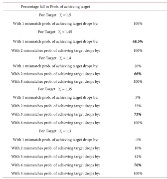
[image:9.595.201.537.339.699.2]The results obtained from the 32 × 32 event-action matrix are summarized in Table 2.2
Table 2. Numerical output obtained from the posited theoretical model for n = 5.
Percentage fall in Prob. of achieving target For Target Y5=1.5
With 1 mismatch prob. of achieving target drops by: 100% For Target Y5=1.45
With 1 mismatch prob. of achieving target drops by: 48.5% With 2 mismatches prob. of achieving target drops by: 100%
For Target Y5=1.4
With 1 mismatch prob. of achieving target drops by: 20% With 2 mismatches prob. of achieving target drops by: 66% With 3 mismatches prob. of achieving target drops by: 100%
For Target Y5=1.35
With 1 mismatch prob. of achieving target drops by: 5% With 2 mismatches prob. of achieving target drops by: 35% With 3 mismatches prob. of achieving target drops by: 73% With 4 mismatches prob. of achieving target drops by: 100%
For Target Y5=1.3
With 1 mismatch prob. of achieving target drops by: -1% With 2 mismatches prob. of achieving target drops by: 10% With 3 mismatches prob. of achieving target drops by: 42% With 4 mismatches prob. of achieving target drops by: 76% With 5 mismatches prob. of achieving target drops by: 100%
2Note: All numbers are hypothetical and intended for illustration only no primary or secondary data
DOI: 10.4236/tel.2018.85065 927 Theoretical Economics Letters The percentage figures (in bold italicized font) represent the percentage drops in likelihood of achieving the best outcome for the particular time path for the highest number of past errors for which that best outcome is achievable. So, for example, for a targeted best possible outcome of 1.45 (i.e. the maximum amount an individual agent can expect to have accumulated at the end of the given plan-ning horizon), the probability of achieving the target drops by 48.5% for a single past prediction error. For two past prediction errors, this probability drops by 100% i.e. the target no longer remains achievable (and would have to be revised downward to the next highest number of 1.40). Again; for a targeted best possi-ble outcome of 1.40, the probability of achieving the target drops by 66% for two past prediction errors. For three past prediction errors, this probability drops by 100% i.e. the target no longer remains achievable (and would have to be revised downward to the next highest number of 1.35); and so on. It is interesting to note that these percentages can be seen to closely approximate the ratio
(
)
* * *
* * *
1 2 1 1
2
p p p
p p p
− − −
= = − ; where *
p is the conviction level predicted by
our theoretical model for a given number of past prediction errors. For 1 predic-tion error *
0.66
p = and 2 1* 0.5
p
− = (corresponding to a 48.5% drop in the
likelihood of achieving the target of 1.45), for 2 prediction errors *
0.75
p = and
*
1
2 0.667
p
− = (corresponding to a 66% drop in the likelihood of achieving the
target of 1.40); for 3 prediction errors *
0.80
p = and 2 1* 0.75
p
− =
(corres-ponding to a 73% drop in the likelihood of achieving the target of 1.35) and for 4 prediction errors *
0.833
p = and 2 1* 0.80
p
− = (corresponding to a 76% drop
in the likelihood of achieving the target of 1.30).
It must be noted that this numerical rendition does not incorporate a massive exogenous shock (reminiscent of the GFC) but is rather a straightforward nu-merical demonstration of how the dynamic time paths would pan out for all possible combinations of event and action and shows how learning might be or-ganically embedded in the temporal evolution process. By incorporating the conviction level (a function of past prediction errors) into the decision process along with the signal generated in each period, an individual agent is better able to identify the optimal path into the future given his/her present location in any intermediate node. For example, if an agent is at the beginning of the fifth (i.e. terminal) period and has only one prediction error till that point, then he can reach at best 1.45 (if he/she selects the risky portfolio and there’s a match of sig-nal with true state in the last period) or, at worst, he/she can reach 1.40 (if he/she selects the risky portfolio and there’s a mismatch of signal with true state in the last period) so will always select risky if target *
1.40
y ≥ . On the other hand, if
DOI: 10.4236/tel.2018.85065 928 Theoretical Economics Letters best (if he/she selects the risky portfolio and there’s a match of signal with true state in the last period) so will need stronger conviction to opt for risky in the last period.
In the next section we firstly present the results of Monte Carlo simulations for two different cases a naïve case (without learning) and an alternative one (with learning). For each of these cases, we have two alternative scenarios one with a massive exogenous shock (reminiscent of the GFC) and the other without a shock. We then discuss the results in detail.
5. Monte Carlo Simulations
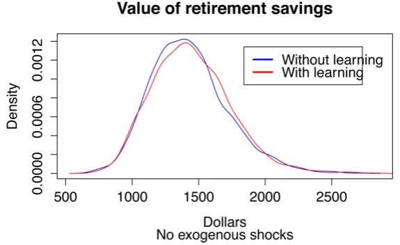
To allow for a more realistic presentation of the implications of the theoretical model the simulations is set up in such a manner that it is representative of an individual who saves for retirement over a 40 year working career. At the end of each month the individual observes the performance of the financial market over the last month and formulates a decision as to how the accumulated assets should be invested for the following month.
As in the theoretical formulation of the model, financial markets have only two states; high returns or low returns. In the simulation the return when the market is “high” is set at 1.0% per month, and when the market is “low” there is a negative return of 0.85% per month. The state of the market in any one period is modeled as a binomial random variable with a 50% probability of a high or low outcome. This effectively gives a slightly positive return to the overall mar-ket in the longer term. There is also a “safe portfolio” and this is set to give a re-turn of 0.1% per month. We consider two cases; one in which the individual “remembers” his past mistakes and the other in which there is no memory of the past. Without memory of past mistakes the individual has no reason not to be optimistic and will thus invest in the risky portfolio in each period. However if past mistakes are remembered then the theoretical model is used to determine if the individual invests in the risky portfolio or the safe portfolio. Without loss of generality an initial investment of $1000 at the beginning of the period is made, and the total reinvested each period. The results of 2000 iterations of the simula-tion are shown is Figure 1.3 The fact that there is little difference in the
situa-tions with and without memory is as expected. The recall of past mistakes does not lead to an advantage in asset selection since it does not provide any advan-tage in predicting the future course of the market.
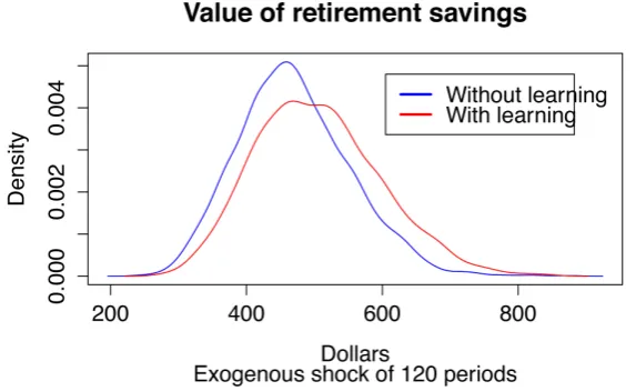
In order to test for the effect of an external shock to the system the simulation is adapted so that a period of “low” returns is forced into the stream of market conditions. Since individuals can experience such as shock at various times in their working career, this string of low returns is inserted randomly into each of the 40 year working careers that are simulated. A shock of 120 consecutive pe-riods of low returns is therefore introduced. All other conditions remain as per
3Note: All numbers are hypothetical and intended for illustration only no primary or secondary data
DOI: 10.4236/tel.2018.85065 929 Theoretical Economics Letters Figure 1. Value of retirement savings, with no external shock.
the first simulation. The results are shown in Figure 2.4
The value of retirement savings falls for both sets of individuals because of the crisis, but the individuals with learning do better. This is not because they are better at predicting the outcome of the market, but because when they expe-rience negative outcomes they adjust by holding the safe portfolio until they have experience enough signals that are correct for them to once again invest in the risky portfolio.
6. Conclusion
The significance of our research is two-fold. Firstly, we have proposed and for-mally derived an extension to the classical dynamic programming model via in-corporation of a Bayesian learning component. Apart from theoretically deriving this extension, we have applied it in the practical context of a retirement savings planning problem whereby an individual agent starts with a given amount in his/her retirement fund and then tries to optimally manage it over a finite time horizon so as to attain a certain minimum target value. The model takes into consideration the risk propensity of the individual agent and yields a trivial solu-tion as per intuisolu-tion if the target minimum value is less than or equal to the maximum value attainable via risk-less investing. The numerical rendition illu-strates that for every past prediction error, the highest possible target end value of the retirement fund would have to be revised downward with an associated drop in the probability of achieving the target for each additional error made. Clearly then, if the individual agent was “learning” from the past errors and the-reby becoming more and more “stringent” in terms of the minimum signal strength required to induce a selection of the risky portfolio, the riskless portfo-lio would be opted for more and more as the number of past errors increased. This would effectively help to “lock in” the fund value to a certain target end value with lower and lower likelihood of any further downward adjustment. Our
4Note: All numbers are hypothetical and intended for illustration only no primary or secondary data
DOI: 10.4236/tel.2018.85065 930 Theoretical Economics Letters Figure 2. Value of retirement savings, with no external shock.
posited “conviction function” allows for a neat integration of the Bayesian learning component with the classical Bellman principle of dynamic optimiza-tion and therefore makes a significant contribuoptimiza-tion to optimizaoptimiza-tion theory. Fi-nally, our Monte Carlo simulations (using hypothetical numbers) clearly illu-strate how the posited model would work in reality, particularly in the event of a large exogenous shock to the investment market (reminiscent of the GFC), the-reby further highlighting its practical significance in financial planning.
References
[1] Wang, C.P., Huang, H.H. and Chen, C.Y. (2015) Does Past Performance Affect
Mutual Fund Tracking Error in Taiwan? Applied Economics, 47, 5476-5490.
[2] Diamond, P.A. and Orszag, P.R. (2005) Saving Social Security. Journal of Economic
Perspectives, 19, 11-32. https://doi.org/10.1257/0895330054048722
[3] Markowitz, H. (1952) Portfolio Selection. The Journal of Finance, 7, 77-91.
[4] Rubinstein, M. (2002) Markowitz Portfolio Selection: A Fifty-Year Retrospective.
The Journal of Finance, 57, 1041-1045. https://doi.org/10.1111/1540-6261.00453
[5] Dybvig, P.H. and Liu, H. (2015) Verification Theorems for Models of Optimal
Consumption and Investment with Retirement and Constrained Borrowing.
Ma-thematics of Operations Research, 19, 11-32.
[6] Bhattacharya, S. and Khoshnevisan, M. (2005) A Proposed Fuzzy Optimal Control
Model to Minimize Target Tracking Error in a Dynamic Hedging Problem with a
Multi-Asset, Best-of Option. Journal of Asset Management, 6, 136-140.
https://doi.org/10.1057/palgrave.jam.2240171
[7] Rust, J. (1987) A Dynamic Programming Model of Retirement Behavior.
http://www.nber.org/books/wise89-1 https://doi.org/10.3386/w2470
[8] Aguirregabiria, V. and Mira, P. (2010) Dynamic Discrete Choice Structural Models:
A Survey. Journal of Econometrics, 156, 38-67. https://doi.org/10.1016/j.jeconom.2009.09.007
[9] Rust, J. and Phelan, C. (1997) How Social Security and Medicare Affect Retirement
Behavior in a World of Incomplete Markets. Econometrica, 65, 781-831.
DOI: 10.4236/tel.2018.85065 931 Theoretical Economics Letters
[10] Sundaram, R.K. (1996) A First Course in Optimization Theory. Cambridge
Univer-sity Press, Cambridge, UK.
[11] Cogley, T. and Sargent, T.J. (2008) Anticipated Utility and Rational Expectations as
Approximation of Bayesian Decision Making. International Economic Review, 49,
185-221. https://doi.org/10.1111/j.1468-2354.2008.00477.x
[12] Lu, K.Y. and Siemer, M. (2013) Learning, Rare Disasters and Asset Prices. Working
Paper in Finance and Economics Discussion Series, Washington, D.C.
[13] Kohlberg, E. and Mertens, J.-F. (1986) On the Strategic Stability of Equilibria.
DOI: 10.4236/tel.2018.85065 932 Theoretical Economics Letters
1. Appendix
1.1. Example: Finite Horizon Decision Making Process and
Conviction Function
In order to obtain a closed form solution we assume that
( )
1 1
0 0 ln
n i n i
t t
i β u c i β c
+ +
= = =
∑
∑
.5Therefore, we can formulate the finite horizondy-namic problem as follows
1 0 ln n i t i c β + = =
∑
(4)
(
)
1
. . t 1 t t;
s t a+ = +R a −c (5)
(
) (
)
(
)
1 if one chooses ;
if one chooses .
c r
t r t
s s t p d R d δ δ − =
(6)
2 0 and 0 .
n
a+ = a =a (7)
In order to solve the above problem, we assume that an individual agent is making his/her decision at period n. At period n, he/she knows for sure that how many mistakes he/she made in the past n−1 periods. Furthermore, we assume
that, one has made
(
n− −1)
k mistakes in the past. In other words, he/shemade correct decisions in k periods. In these k periods, he/she may have made both risky and safe investments. Suppose, he/she makes successful risky invest-ment for x periods; and he/she makes safe investinvest-ment for k−x periods. Thus his initial asset accumulation at period n−1 is as follows:
(
) (
)
1 1 1
k x x
n r s
a− = +δ +δ − a (8)
In period n, the value function (following from Bellman’s optimal principal) one faces is as follows:
( )
( )
1 0 1
max ln
n
n
n n n
c V a =
β
c +V a+ (9)Similarly, in period n−1, the value function will be as follows:
( )
( )
1
2 1 1 1
max ln
n
n
n n n
c− V a− =
β
c− +V a (10)Both Equations (9) and (10) are key to find out the Bellman’s Optimal prin-ciple. The solutions of Equations (9) and (10) are discussed in the next section.
1.2. Solution
One can easily solve Equations (9) and (10) with the help of Equations (5) to (8). The optimal solutions are provided as follows:
(
)
(
1)
* 1 1 1 1 n n R a c β β − − + =
+ + (11)
(
)(
)
(
)
1* 1 1
1 1
n n
R a
a β β
β β
−
+ +
=
+ + (12)
5Note that, this assumption is standard in the literature of economics where the utility function is
DOI: 10.4236/tel.2018.85065 933 Theoretical Economics Letters
(
)
* 1 1 n n R a c β + =+ (13)
(
)
* 1 1 1 n n R a a β β + + =+ (14)
By using Equations (8), (12) and (14) we obtain the asset value in period
1
n+ , which is as follows:
(
) (
)(
)
(
) (
) (
)
* 1
1 1 1
1 1
1 1 1
k x x
n r s
R R
a β β β δ δ a
β β β
− +
+ + +
= + +
+ + + (15)
If one chooses to invest in the risky asset for two successive periods (provided that he/she does not make any mistake) then the Equation (15) will be as follows:
(
)
(
)
(
)
(
) (
)
2 2 * 1 1 1 1 1 1 1 ct r x k x
n r s
p a a β δ δ δ β β − + + − = + +
+ + (16)
On the other hand, if one chooses to invest in the safe asset for two successive periods (provided that he/she does not make any mistake) then the Equation (15) will be as follows:
(
)
(
) (
) (
)
2 2 * 1 1 1 1 1 1 k x x sn r s
a β δ δ δ a
β β
− +
+
= + +
+ + (17)
Note that, following from Proposition 1(B), the value of c t
p when t= −n 1
will be
1
n k
n k
−
− + . Thus comparing Equations (16) and (17), one will invest in
risky asset if the following condition is met:
(
)
(
)
** 1 1 ct r s
r s
r s s
r s p n k n k n k k δ δ δ δ
δ δ δ
δ δ − ≥ − ⇒ ≥ − + − − ⇒ ≡ ≥ − (18)
Equation (18) develops the following Lemma: Lemma 1 There exists **
0
k > such that if **
k<k then an individual
deci-sion maker will choose to invest in the risky asset. On the other hand if ** k≥k
then an individual investor will invest in the safe asset. Proof. The proof follows from Equation (18).
Lemma 1 implies that there exists a critical level for the periods of correct de-cision making, **
k , in conjunction with conviction function such that if ** k<k
then an individual decision maker invests in the risky asset since the expected benefit from investing on such asset will be higher. However, the reverse will be true if **
k≥k i.e. in this case safe investment gives higher return.
Interesting question one might ask is that how the above outcome based on conviction function differs from the outcome based on Bayesian learning. The answer lies on what values α will take based on Bayesian learning only (follows
by Definition 1) when one chooses to invest on risky asset ( r t
DOI: 10.4236/tel.2018.85065 934 Theoretical Economics Letters case, α takes the following value:
1
1 if and signal is matched ; 2
0 otherwise.
p g
α
>
=
(19)
However, with the conviction function one faces the following value of α
{ }
(
)
1 c 1 2 | signal g is matched,
t
p p k
α = − > = (20)
Here, =
{ }
k refers past history where k number of periods an individualinvestor makes correct decisions in making investment on risky asset. Equation (19) will be special case of conviction function (follows from Proposition 1(A) and 1(C)). Thus without conviction function α will be either overestimated or