An Estimation of the Capital Growth Rate in
Business Activities
Bartosz Kurek
Accounting Department, Cracow University of Economics, Krakow, Poland Email: kurekb@uek.krakow.pl
Received March 2,2012; revised March 15, 2012; accepted April 21, 2012
ABSTRACT
The aim of the paper is to empirically assess whether capital growth rates (defined as in the paper) realized by compa- nies constituting Standard & Poor’s indices: S&P 600, S&P 400 and S&P 500 were higher in years prior to crisis, i.e. in years: 2007, 2006, 2005 than the average growth rates in preceding 5-year periods, i.e. in periods: 2002-2006, 2001-2005 and 2000-2004. A statistical test concerning the differences between means was used as a research method. In order to achieve that 9 hypotheses were tested in total. The further purpose of this paper is to estimate capital growth rates for every index in each of the years from 2000 up to 2007, as well as in 5- and 8-year periods. In total 40 confi- dence intervals for capital growth rates were constructed in order to achieve that goal. M. Dobija’s theory of capital was used as a background for a research. According to that theory capital is an abstract ability to perform labor. Homoge- neous capital is embodied in heterogeneous assets. Capital is subdued to a number of laws: 1) the conservation principle and 2) the dispersion principle. These laws form the fundamentals of the theory of capital. The concentration of capital in any particular time moment is described in the form of the equation, where initial capital is influenced by the three factors: a natural potential of growth, a spontaneous diffusion and an inflow of capital by human labor and management. The natural potential of growth may be estimated by a properly defined ROA index. Realized ROA by a single com- pany in a particular time period is a random number. However, in a large sample of companies, the average ROA index over a long time period concentrates around the natural potential for growth. The research shows that in most cases the capital growth rates were statistically higher in years prior to crisis than the average growth rates in preceding 5-year periods. Similarly—in most cases—the average rate of return on assets in each of the indices was increasing from year to year in nominal terms. That increased return on assets might strengthen the believes of investors that higher and higher profits are achievable on a regular basis. However, it seems that investors did not acknowledge that returns will float towards the average ultimately as the theory of capital describes.
Keywords: Capital; Capital Growth Model; Return on Assets
1. Introduction
P. Viernimmen et al. ([1]: p. 8) claim that “The origin of the financial crisis that began in 2007 is a textbook case. What we have here are greedy investors seeking increas- ingly higher returns, who are never satisfied when they have enough and always want more”. Following the two recent publications in Modern Economy, i.e. [2,3], which are based on the model of capital and the deterministic risk premium concept, the question arises whether the need for such returns was justified by higher than aver- age accounting returns of companies at the stock market. It may be claimed that companies which are well managed are a benchmark for investors, and if their stock is traded on the stock exchange, the ownership of them is easily accessible for everybody. Especially it may be argued that companies constituting such indices as: Stan- dard & Poor’s SmallCap 600, Standard & Poor’s MidCap
400, Standard & Poor’s 500 are benchmarks for well managed companies in developed countries, such as, but not limited to, USA. Specifically as Standard & Poor’s [4] claims: “The S&P SmallCap 600 covers approximately 3% of the domestic equities market. Measuring the small cap segment of the market that is typically renowned for poor trading liquidity and financial instability, the index is designed to be an efficient portfolio of companies that meet specific inclusion criteria to ensure that they are investable and financially viable”. Similarly Standard & Poor’s [5] claims that: “The S&P MidCap 400® provides
that: “The S&P 500® has been widely regarded as the
best single gauge of the large cap US equities market since the index was first published in 1957 (…). The in-dex includes 500 leading companies in leading industries of the US economy, capturing 75% coverage of US equi-ties”.
The aim of the paper is to empirically assess via statis- tical test concerning differences between means whether capital growth rates (defined as in the paper) realized by companies constituting Standard & Poor’s indices: Stan- dard & Poor’s SmallCap 600, Standard & Poor’s MidCap 400 and Standard & Poor’s 500 were higher in years prior to crisis, i.e. in years: 2007, 2006, 2005 than the average growth rates in preceding 5-year periods, i.e. in periods: 2002-2006, 2001-2005 and 2000-2004. In total 9 hypotheses were tested.
Capital growth rates are then estimated for every index in each of the years from 2000 up to 2007, as well as in five and eight year periods.
2. Capital and the Capital Growth Model
The term “capital” has been widely used in economics, accounting and finance. However, researchers have not ever reached consensus on the meaning of that concept. Controversies concerning the nature and definitions of capital have been noted already by I. Fisher [7], E. von Böhm-Bawerk [8], E. Majewski ([9]: p. 8) and S. Skrzy- pek [10] and numerous other academics and profession-als. One of capital researchers, C. Bliss ([11]: p. 7), even wrote: “when economists reach agreement on the theory of capital they will shortly reach agreement on every- thing. Happily, for those who enjoy a diversity of views and beliefs, there is very little danger of this outcome. Indeed, there is at present not even agreement as to what the subject is about”.A number of researchers noticed that capital is an ab- stract concept, e.g. I. Fisher compared capital to an ab- stract economic power. Y. Ijiri ([12]: p. 62) noted that capital is abstract, homogeneous and aggregated, whilst resources are concrete, heterogeneous and disaggregated. Likewise M. Dobija ([13]: p. 89) claims that “In eco-nomic language, capital is an ecoeco-nomic power, an ability of doing work, although academics have not been fully aware of this connection. Much trouble with real econo- mies, and economic theories as well, has its roots in the lack of reconciliation of the capital concept in economics. In physics energy is defined as the capacity to do work and thermodynamics is the field, in which the applica- tions of energy and heat are thoroughly studied. Capital in economics is the same abstract concept as energy in physics but considerations are limited to adequate do- mains.” In that understanding, capital is embodied in assets (physical or intangible) and its concentration com-
prises the value of assets. At this moment it is important to note that energy in physics, although defined also as an ability to perform labor, is a different concept to capi- tal. Laws of energy cannot be literally translated into economy, but have to be appropriately adjusted. Espe- cially the second law—presented below—should be sepa- rated from the second law of energy and entropy concept, since the term entropy should only apply to thermody-namics and should not be transferred as an analogy to other areas (compare [14]).
Capital is therefore subdued to such laws, as:
The conservation principle (the total amount of capi-tal remains constant in an isolated system, i.e. the ini-tial capital can only be changed or transformed but never created);
The dispersion principle (capital decreases its concen- tration over time, i.e. the initial value of capital spon- taneously and randomly declines);
The capital growth principle (described by the capital growth model which stems from the assumption that economy is a non-zero game).
Capital growth model describes the concentration of capital at a point in time. In companies that continue their operations, capital grows according to the Equation (1) ([15]: p. 133)1:
1, , , 0
p s M t
t s p M t
C C e , (1)
where:
Ct0—the beginning concentration of capital [expressed
in monetary terms] in the time moment t0,
Ct1,s,p,M—the ending concentration of capital [ex-
pressed in monetary terms] in the time moment t1, which has been subdued to natural dispersion “s” (risk), risk premium “p” and a management variable “M” through the time period ∆t,
S—dispersion variable (risk) [expressed as 1/year],
P—risk premium, p = E(s) [expressed as 1/year],
M—management variable [expressed as 1/year], ∆t—time period between time moments: t0 and t1 [ex- pressed in years].
According to M. Dobija [3] “the variables s and m
represent active work of the natural forces (–s) and the active outer work that can restrain the dispersion (m) (…) the constant p symbolizes a potential. The potential p can yield fruit, provided the diffusion s is counterbalanced by the work m”. The author claims that the ex ante size of the potential p equals to 8%/yr. That potential represents the fair capital growth rate. Modified return on assets ratio may serve as proxy for risk premium estimation and as empirical research done at the 20 year period suggests, the yearly size of ex post p for average risk level condi- tions may be described as the 99.9% confidence interval:
(8.08%/yr ; 8.74%/yr) [16].
Capital will grow and increase its concentration only if: “p – s + M > 0”. That condition represents at the same time ex post rate of return on invested capital, and also at the same time capital growth rate expressed in [1/year].
Recalling that capital is embodied in assets the Equa- tion (2) may be stated ([16]: p. 95):
1, , , 0
p s M t
e
t s p M t
A A , (2)
where:
At1,s,pM—the net cost of assets in the time moment t1 (these assets embody capital, that is subdued to natural dispersion “s” (risk), risk premium “p” and a manage- ment variable “M” through the time period of ∆t = t1– t0, e.g. 1 year);
At0—the net cost of assets in the time moment t0.
Further, knowing that “er ≈ 1 + r”, the Equation (2) may be rearranged into Equation (3):
1, , , 0 1
t s p M t
A A p s M t. (3)
The reconciliation of units and their dimensions used in the Equation (3) clearly shows that the value of assets,
i.e. the concentration of capital in resources, is expressed in monetary units in the beginning and in the end of a period under consideration. That is proven by the Equa- tion (4):
$ $ 1 1 1 yr 1 y
r 1 yr
yr . (4) In the formula (3), factors “p” (risk premium), “s” and “M”, taken together, create an empirical growth rate, which is expressed in [1/year] terms. That growth rate is in fact the rate of return on capital in a one-year period or the rate of return on assets if the previously described understanding of capital is accepted. Thus, by skipping factors “p”, “s” and “M”, the Equation (5) may be writ- ten:
1 0 1 year ,
t t
A A
A t
1, 0
ROAt t t
(5)
where:
At1—the net cost of assets in the time moment t1,
At0—the net cost of assets in the time moment t0,
∆t = t1– t0,
ROAt1,∆t—the rate of return on capital embodied in
assets calculated in t1 time moment realized in the time period ∆t.
The increase in concentration of capital embodied in assets “At1 – At0” equals to the realized income in a con-
sidered period “I∆t”. Since business processes are con- tinuous processes rather than discrete, it seems more ap- propriate to compare the realized income “I∆t” to the av- erage value of capital (equity or debt that is embodied in assets) in a considered period “Aav”. The change in the
denominator results in the Equation (6):
1,
0 1
ROA 1 2
t t t
t t
I
A A t
, (6)
where:
I∆t—the realized income before extraordinary items in the period ∆t,
At1, At0,∆t and ROAt1,∆t as above.
The category of income to be used in the numerator of the formula number (6) should represent the normal op- erating conditions of each company. Therefore the im- pact of extraordinary items should be eliminated. As a result one can use Pretax Income category. Another ad- vantage of that formula is that it is an income level be- fore distribution of profit i.e. before dividends and taxes were paid. Summing up, Pretax Income category relates to the growth of capital in a particular period for normal risk level conditions.
3. Research Hypotheses
As M. Dobija suggests in his quoted publications, i.e. [2] and [3], as well as in numerous other, the potential for capital growth is a constant value of 8% per year. The research suggests that this potential is not realized as a rate of return on capital/assets for every company in each subsequent year [16,17]. Rather, the eight percent em- pirical growth rate is realized in large populations in av- erage risk level conditions in long time periods. Compa- nies in certain periods randomly realize higher or lower capital growth rate than the potential specified by M. Dobija in his model, however in the long term in large populations, average empirical capital growth rate will float towards the average. Therefore it may be stated that investors should not drain companies in more prosperous periods. They should rather allow firms to accumulate capital for times of crisis, as these periods will be fol- lowed by poorer ones.
The paper addresses a question, whether average ROA realized by companies in the years prior to the recent crisis were higher than the average rates in preceding five year periods. That might have led investors to seek for higher returns. The result was the recent textbook crisis as P. Viernimmen et al. claims.
The researched sample consists of companies consti- tuting Standard & Poor’s SmallCap 600, Standard & Poor’s MidCap 400, Standard & Poor’s 500 indices on 31st January 2008. Audited, filed financial statements
come from years 1999-20072. These financial statements
were obtained from COMPUSTAT database (North America set, software: Research Insight version 8.3,
0.75). t—value of the test statistics (t-Student distribution), Null hypotheses are presented in Table 1, whereas
al-ternative hypotheses are presented in Table 2.
df—modified degrees of freedom,
s—standard deviation, The average rates of return on assets in the researched
time periods are presented in Table 3.
n—number of observations,
X—arithmetic average from the sample. Subscripts 1 and 2 relate to compared populations.
In order to verify all of the presented hypotheses a test of the differences between two population means was applied—Equation (7), with the usage of the modified degrees of freedom—Equation (8) [18]:
Table 4 includes the overall number of observations in
each index according to the period. Table 5 includes
values of t-statistics rounded to the fourth digit after a comma and the number of modified degrees of freedom rounded to the nearest unit. For the one-sided test the critical t-value (t-Student distribution) for significance levels of: α = 0.100, α = 0.050, α = 0.025, α = 0.010, α = 0.005 and the number of degrees of freedom approaching ∞, equals to: ±1.282, ±1.645, ±1.960, ±2.326, ±2.576 respectively (plus sign if the order of averages in the numerator is as in null hypotheses). Table 6 presents the
statistical decisions whether the researched data rejects the null hypothesis or whether the data fails to reject it at a given significance level.
1 2 2 2 1 2 21 2
X X
t
s s
n n
, (7)
2 2 2 1 2 1 2
2 2
2 2
2 2
1 2
s s
n n
s n
n n
1 1
df
s n
, (8)
where:
Table 1. Null hypotheses.
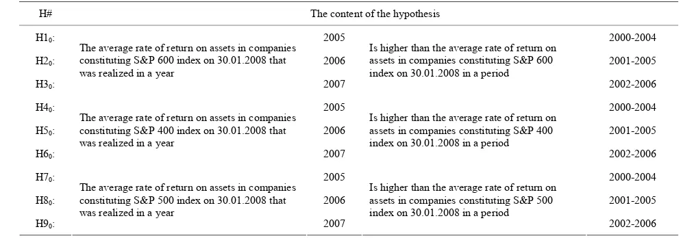
H# The content of the hypothesis
H10: 2005 2000-2004
H20: 2006 2001-2005
H30:
The average rate of return on assets in companies constituting S&P 600 index on 30.01.2008 that was realized in a year
2007
Is lower than or equal to the average rate of return on assets in companies constituting S&P 600 index on 30.01.2008 in a period
2002-2006
H40: 2005 2000-2004
H50: 2006 2001-2005
H60:
The average rate of return on assets in companies constituting S&P 400 index on 30.01.2008 that was realized in a year
2007
Is lower than or equal to the average rate of return on assets in companies constituting S&P 400 index on 30.01.2008 in a period
2002-2006
H70: 2005 2000-2004
H80: 2006 2001-2005
H90:
The average rate of return on assets in companies constituting S&P 500 index on 30.01.2008 that was realized in a year
2007
Is lower than or equal to the average rate of return on assets in companies constituting S&P 500 index on 30.01.2008 in a period
[image:4.595.43.540.563.737.2]2002-2006
Table 2. Alternative hypotheses.
H# The content of the hypothesis
H10: 2005 2000-2004
H20: 2006 2001-2005
H30:
The average rate of return on assets in companies constituting S&P 600 index on 30.01.2008 that was realized in a year
2007
Is higher than the average rate of return on assets in companies constituting S&P 600 index on 30.01.2008 in a period
2002-2006
H40: 2005 2000-2004
H50: 2006 2001-2005
H60:
The average rate of return on assets in companies constituting S&P 400 index on 30.01.2008 that was realized in a year
2007
Is higher than the average rate of return on assets in companies constituting S&P 400 index on 30.01.2008 in a period
2002-2006
H70: 2005 2000-2004
H80: 2006 2001-2005
H90:
The average rate of return on assets in companies constituting S&P 500 index on 30.01.2008 that was realized in a year
2007
Is higher than the average rate of return on assets in companies constituting S&P 500 index on 30.01.2008 in a period
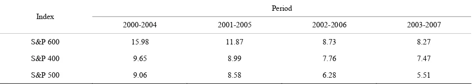
Table 3. Average rates of return on assets in each index ac- cording to the period.
Index S&P 600 S&P 400 S&P 500
Period ROA [%/yr]
2000-2004 6.19 8.02 8.19
2001-2005 6.74 8.15 8.11
2002-2006 7.81 8.81 9.05
[image:5.595.57.287.113.251.2]2005 8.68 9.64 10.70 2006 8.86 10.11 10.97 2007 8.02 11.11 11.59
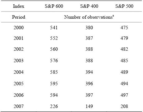
Table 4. The number of observations in each index accord- ing to the period.
Index S&P 600 S&P 400 S&P 500 Period Number of observationsa
2000-2004 2814 1937 2410
2001-2005 2868 1953 2429
2002-2006 2910 1963 2447
2005 595 396 494 2006 594 397 497 2007 226 149 208 aAccording to data availability.
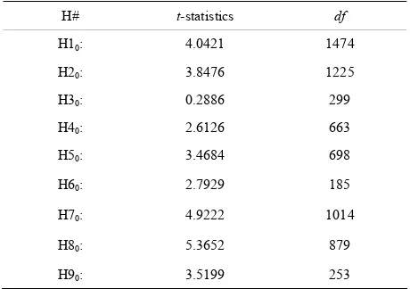
Table 5. T-statistics and the numbers of modified degrees of freedom for each of the hypotheses.
H# t-statistics df
H10: 4.0421 1474
H20: 3.8476 1225
H30: 0.2886 299
H40: 2.6126 663
H50: 3.4684 698
H60: 2.7929 185
H70: 4.9222 1014
H80: 5.3652 879
H90: 3.5199 253
The statistical hypotheses testing clearly showed that eight out of nine null hypotheses were rejected on the basis of researched data and only one null hypotheses was not rejected. The average rates of return on assets in companies constituting S&P 600 index on 30.01.2008 that were realized in a year 2005 and 2006 were statisti- cally higher than in periods 2000-2004 and 2001-2005
Table 6. Decision on the rejection of null hypotheses on the basis of researched data.
α H#
0.100 0.050 0.025 0.010 0.005
H10: YES YES YES YES YES
H20: YES YES YES YES YES
H30: NO NO NO NO NO
H40: YES YES YES YES YES
H50: YES YES YES YES YES
H60: YES YES YES YES YES
H70: YES YES YES YES YES
H80: YES YES YES YES YES
H90: YES YES YES YES YES
respectively. Similarly the average rates of return on as- sets in companies constituting S&P 400 index on 30.01. 2008 that were realized in a year 2005, 2006 and 2007 were statistically higher than in periods 2000-2004, 2001-2005 and 2002-2006 respectively. The same ap- plies for companies constituting S&P 500 index on 30.01. 2008—the average rates of return on assets in companies constituting that index on 30.01.2008 that were realized in a year 2005, 2006 and 2007 were statistically higher than in periods 2000-2004, 2001-2005 and 2002-2006 respectively. Only the third hypothesis cannot be rejected on the basis of presented data—the average rate of return on assets in companies constituting S&P 600 index on 30.01.2008 that was realized in a year 2007 was lower than or equal to the average rate of return on assets that was realized in a period 2002-2006. The 2007 capital growth rate equaled to 8.02%/yr in that sample, whereas the one realized in the period 2002-2006 equaled to 7.81%/yr, which is still higher in nominal values.
It is worth to mention that year by year average capital growth rates increased for companies constituting S&P 400 and S&P 500 indices, starting from 9.64%/yr in 2005 though 10.11%/yr in 2006 ending with 11.11%/yr in 2007 in case of the former and starting from 10.70%/yr in 2005 though 10.97%/yr in 2006 ending with 11.59%/yr in 2007 in case of the latter. Average capital growth rate in companies constituting S& P600 index equaled to 8.68%/yr in 2005 and increased to 8.86%/yr in 2006, after which it dropped to 8.02%/yr in 2007.
4. Capital Growth Rate Estimation
[image:5.595.58.287.289.427.2] [image:5.595.57.287.477.639.2]sample consisting of a particular index (S&P 600, S&P 400 and S&P 500) may serve as an estimator for capital growth rate in the population of small, medium and large well managed companies respectively. According to the central limit theorem the formula based on the standard normal distribution may be used to estimate population mean, when sampling from any distribution with un- known variance and when sample size is large. The numbers of observations in each index in each of years under consideration are presented in Table 7. It may be
claimed that the sample sizes are large.
The two-sided confidence interval for the population capital growth rate is constructed according to the for- mula number (9) (compare [19]):
1, ; 1, ;
ROAt t n ROA ROAt t n
s
P z
n 1
s z
n
,
(9) where:
z—value of the test statistics (normal distribution),
s—standard deviation,
n—the number of observations,
1, ;
t t n—average rate of return on capital embod- ied in assets calculated in t1 time moment (the end of the calendar year for which the average ROA is calculated) realized in the time period ∆t (the calendar year for which the average ROA is calculated) from n observa- tions in a particular index,
ROA
ROA—capital growth rate in the population under consideration;
1–α—confidence interval.
Average rates of return on assets for each year and each index are presented in Table 8, whereas standard
deviations are presented in Table 9.
Confidence intervals for capital growth rates in each index in each of the years for the degree of confidence equal to 0.99 are presented in Table 10 (1-year periods),
in Table 11 (5-year periods) and in Table 12 (8-year
periods). Relative precisions of estimations are included in Tables 13-15 respectively.
Relative precisions of estimations in case of 1-year pe- riods it is higher than 10% and as a result estimation is completely wrong. That proves the need for long time horizons research. In case of 5-year periods relative pre- cisions of estimations only in two situations are above 10%. In all other situations these are below 10% but still above 5%, which is not satisfactory, as it cannot be claimed that estimation is safe and fully acceptable.
Even in the case of 8-year periods relative precisions of estimations are above 5% in case of the degree of con-fidence equal to 99%.
[image:6.595.308.538.111.291.2]By limiting the degree of confidence to 90%, one can achieve relative precision of estimations below 5% for
Table 7. The number of observations in each index in each year.
Index S&P 600 S&P 400 S&P 500 Period Number of observationsa
2000 541 380 475 2001 552 387 479 2002 560 388 482
2003 576 388 485
2004 585 394 489 2005 595 396 494
2006 594 397 497 2007 226 149 208 aAccording to data availability.
Table 8. Average rates of return on assets in each index according to the year.
Index S&P 600 S&P 400 S&P 500
Period ROA [%/yr]
2000 6.00 9.03 11.18 2001 3.40 6.83 6.28 2002 4.98 6.47 6.19
2003 7.70 8.51 7.78
[image:6.595.308.537.341.517.2]2004 8.89 9.26 9.52 2005 8.68 9.64 10.70 2006 8.86 10.11 10.97 2007 8.02 11.11 11.59
Table 9. Standard deviations of the average rates of return on assets in each index according to the year.
Index S&P 600 S&P 400 S&P 500 Period Standard deviation [%/yr]
2000 29.12 14.23 13.95 2001 22.04 13.93 20.04 2002 14.80 11.93 14.03 2003 18.83 15.48 10.28
2004 13.42 9.58 9.22
[image:6.595.309.537.557.734.2]Table 10. Confidence intervals for capital growth rate (1-year periods).
Index S&P 600 S&P 400 S&P 500
Period Confidence intervals for the degree of confidence equal to 0.99
2000 P [2.78%/yr < ROA < 9.23%/yr] = 0.99 P [7.14%/yr < ROA < 10.91%/yr] = 0.99 P [9.53%/yr < ROA < 12.83%/yr] = 0.99
2001 P [0.98%/yr < ROA < 5.81%/yr] = 0.99 P [5.00%/yr < ROA < 8.65%/yr] = 0.99 P [3.92%/yr < ROA < 8.63%/yr] = 0.99
2002 P [3.37%/yr < ROA < 6.59%/yr] = 0.99 P [4.91%/yr < ROA < 8.03%/yr] = 0.99 P [4.55%/yr < ROA < 7.84%/yr] = 0.99 2003 P [5.47%/yr < ROA < 9.52%/yr] = 0.99 P [6.49%/yr < ROA < 10.53%/yr] = 0.99 P [6.58%/yr < ROA < 8.98%/yr] = 0.99
2004 P [7.46%/yr < ROA < 10.32%/yr] = 0.99 P [8.02%/yr < ROA < 10.50%/yr] = 0.99 P [8.44%/yr < ROA < 10.59%/yr] = 0.99
2005 P [7.44%/yr < ROA < 9.91%/yr] = 0.99 P [8.24%/yr < ROA < 11.04%/yr] = 0.99 P [9.61%/yr < ROA < 11.79%/yr] = 0.99 2006 P [7.69%/yr < ROA < 10.03%/yr] = 0.99 P [8.85%/yr < ROA < 11.36%/yr] = 0.99 P [9.79%/yr < ROA < 12.16%/yr] = 0.99
[image:7.595.53.539.101.287.2]2007 P [6.27%/yr < ROA < 9.77%/yr] = 0.99 P [9.10%/yr < ROA < 13.11%/yr] = 0.99 P [9.82%/yr < ROA < 13.35%/yr] = 0.99
Table 11. Confidence intervals for capital growth rate (5-year periods).
Index S&P 600 S&P 400 S&P 500
Period Confidence intervals for the degree of confidence equal to 0.99
2000-2004 P [5.20%/yr < ROA < 7.18%/yr] = 0.99 P [7.24%/yr < ROA < 8.79%/yr] = 0.99 P [7.44%/yr < ROA < 8.93%/yr] = 0.99 2001-2005 P [5.94%/yr < ROA < 7.54%/yr] = 0.99 P [7.42%/yr < ROA < 8.88%/yr] = 0.99 P [7.42%/yr < ROA < 8.81%/yr] = 0.99
2002-2006 P [7.13%/yr < ROA < 8.49%/yr] = 0.99 P [8.12%/yr < ROA < 9.49%/yr] = 0.99 P [8.49%/yr < ROA < 9.62%/yr] = 0.99
[image:7.595.61.537.313.422.2]2003-2007 P [7.75%/yr < ROA < 9.14%/yr] = 0.99 P [8.82%/yr < ROA < 10.25%/yr] = 0.99 P [9.38%/yr < ROA < 10.48%/yr] = 0.99
Table 12. Confidence intervals for capital growth rate (8-year periods).
Index S&P 600 S&P 400 S&P 500
Period Confidence intervals for the degree of confidence equal to 0.99
2000-2007 P [6.31%/yr < ROA < 7.72%/yr] = 0.99 P [8.10%/yr < ROA < 9.28%/yr] = 0.99 P [8.56%/yr < ROA < 9.67%/yr] = 0.99
Table 13. Relative precision of estimation in % (1-year periods, degree of confidence equals to 0.99).
Period Index
2000 2001 2002 2003 2004 2005 2006 2007
S&P 600 53.72 71.15 32.37 26.96 16.08 14.25 13.21 21.81
S&P 400 20.84 26.71 24.12 23.78 13.42 14.50 12.41 18.07
S&P 500 14.75 37.58 26.57 15.45 11.29 10.17 10.79 15.24
Table 14. Relative precision of estimation in % (5-year periods, degree of confidence equals to 0.99).
Period Index
2000-2004 2001-2005 2002-2006 2003-2007
S&P 600 15.98 11.87 8.73 8.27
S&P 400 9.65 8.99 7.76 7.47
[image:7.595.57.539.535.620.2] [image:7.595.59.539.650.736.2]indices S&P 400 and S&P 500, which is a level of safe and fully acceptable estimation (Tables 16 and 17). An-
other possibility is to increase the size of the sample, which was done in [16,17,20].
5. Conclusions
Capital in economy—according to the contemporary approach—is understood as an abstract homogeneous ability to perform labor. Capital is embodied in assets, which are concrete and heterogeneous. The concentration of capital comprises the value of assets. Capital is sub- dued to a number of laws, such as: the conservation prin- ciple the dispersion principle and the capital growth principle. The conversion principle states that the total amount of capital remains constant in an isolated system. The increase of initial capital in an enterprise may only be caused by the exchange at the free, efficient market. The dispersion principle states that the initial value of capital spontaneously and randomly declines.
[image:8.595.57.286.430.500.2]Capital growth principle stems from the assumption that economy is a non-zero game. According to M. Do- bija the fair capital growth rate in an average risk level conditions equals to the potential of 8%. The potential is one of the three factors that condition the concentration of capital in a particular time moment. The remaining
Table 15. Relative precision of estimation in % (8-year pe- riods, degree of confidence equals to 0.99).
Index Period 2000-2007
S& P600 10.10
S&P 400 6.82
[image:8.595.58.287.550.624.2]S&P 500 6.09
Table 16. Confidence intervals for capital growth rate (8- year periods).
Confidence intervals for the degree of confidence equal to 0.90
Index Period 2000-2007
[image:8.595.58.285.664.734.2]S&P 600 P [6.56%/yr < ROA < 7.47%/yr] = 0.90 S&P 400 P [8.31%/yr < ROA < 9.07%/yr] = 0.90 S&P 500 P [8.76%/yr < ROA < 9.46%/yr] = 0.90
Table 17. Relative precision of estimation in % (8-year pe- riods, degree of confidence equals to 0.90).
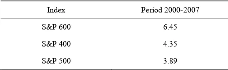
Index Period 2000-2007
S&P 600 6.45
S&P 400 4.35
S&P 500 3.89
two factors are natural dispersion and management vari- able. These three factors determine the rate of return on invested capital, which is a random number for a par- ticular company.
The potential may be empirically estimated. Capital average growth rates of companies operating in average level conditions fluctuate around the potential, assuming that large populations over long time periods are tested. Individual capital growth rates are random numbers, i.e.
cannot be forecasted with certainty. The estimation of the potential is in fact the estimation of the fair average capital growth rate in large populations. The theory of capital states that the higher capital growth rates in some periods will be followed by the lower growth rates in other periods.
Therefore higher capital growth rates in some periods cannot be used to justify the drain of profits from com- panies, as in other periods returns will reverse and move towards long term average. P. Viernimmen et al. claimed that the 2007 crisis was a textbook case, where greedy investors sought increasingly higher returns and were never satisfied when they had enough. Empirical re- search suggests that capital growth rates in years prior to crisis were higher than the average capital growth rates in the preceding years. The nine hypotheses were tested in order to prove the assumption. In case of Standard & Poor’s MidCap 400 index and Standard & Poor’s 500 index the capital growth rates that were realized in years prior to crisis, i.e. in years: 2007, 2006, 2005 were statis- tically higher than the average growth rates in preceding 5-year periods, i.e. in periods: 2002-2006, 2001-2005 and 2000-2004 respectively. In case of Standard & Poor’s SmallCap 600 index the capital growth rates that were realized in years prior to crisis, i.e. in years: 2006, 2005 were statistically higher than the average growth rates in preceding 5-year periods, i.e. in periods: 2001-2005 and 2000-2004 respectively. Only in case of Standard & Poor’s SmallCap 600 index the realized capital growth rate in year 2007 was not statistically higher than the average growth rates in a period 2002-2006.
industries of the US economy. On the other hand S&P 600 index covers small cap segment of the market, which is characterized by poor trading liquidity and financial instability. S&P 400 index is in between the two indices. It is particularly important to learn that capital growth rates fluctuate around the potential of growth. That know- ledge may protect individual investors—citizens—from losses. Greedy institutional investors frequently tempt citizens with constant higher than average returns. The past pattern of returns may not continue in future periods. The constant increase in capital growth rates may even act as a warning sign. The theory of capital explains the phenomenon—capital growth rates fluctuate around the potential of growth.
REFERENCES
[1] P. Viernimmen, P. Quiry, M. Dallocchio, Y. Le Fur and A. Salvi, “Corporate Finance: Theory and Practice,” John Wiley & Sons Ltd., Chichester, 2009.
[2] M. Dobija, “Abstract Nature of Money and the Modern Equation of Exchange,” Modern Economy, Vol. 2, No. 2, 2011, pp. 142-152. doi:10.4236/me.2011.22019
[3] M. Dobija, “Labour Productivity vs Minimum Wage Level,”
Modern Economy, Vol. 2, No. 5, 2011, pp. 780-787. doi:10.4236/me.2011.25086
[4] “S&P Indices: The S&P MidCap 600,” Access on 2 Janu- ary 2012.
http://www.standardandpoors.com/indices/sp-smallcap-6 00/en/eu/?indexId=spusa-600-usduf--p-us-s-- [5] “S&P Indices: The S&P MidCap 400,” Access on 2
Janu-ary 2012.
http://www.standardandpoors.com/indices/sp-midcap-400 /en/eu/?indexId=spusa-400-usduf--p-us-m--
[6] “S&P Indices: The S&P MidCap 500,” Access on 2 Janu- ary 2012.
http://www.standardandpoors.com/indices/sp-500/en/eu/? indexId=spusa-500-usduf--p-us-l--
[7] I. Fisher, “The Nature of Capital and Income,” Augustus M. Kelly Publisher, New York, 1965, pp. 53-57. [8] E. von Böhm-Bawerk, “Capital and Interest, Vol. 2: Posi-
tive Theory of Capital,” Libertarian Press, South Holland, 1959, pp. 16-66.
[9] E. Majewski, “Capital: The Set of Core Phenomena and Concepts in Economy,” 4th Edition, E. Wende i ska, Wars- zawa, 1914.
[10] S. T. Skrzypek, “The Concept of Capital in Literature,” Nakł. Towarzystwa Naukowego, Pomerania, 1939. [11] C. Bliss, “Capital Theory and the Distribution of Income,”
North-Holland Publishing Company, Oxford 1975. [12] Y. Ijiri, “Segment Statements and Informativeness Meas-
ures: Managing Capital vs Managing Resources,” Account- ing Horizons, Vol. 9, No. 3, 1995, pp. 55-67.
[13] M. Dobija, “Abstract Nature of Capital and Money” In: L. M. Cornwall, Ed., New Developments in Banking and Finance, Nova Science Publishers, Inc., New York, 2007, pp. 89-114.
[14] F. L. Lambert, “Shuffled Cards, Messy Desks, and Dis-orderly Dorm Rooms—Examples of Entropy Increase? Nonsense!” The Journal of Chemical Education, Vol. 76, No. 10, 1999, pp. 1385-1387. doi:10.1021/ed076p1385 [15] M. Dobija, “Fair Value as a Criterion of Truth in Eco-
nomic Theory” In: W. Adamczyk, Ed., Dążenie do Prawdy w Naukach Ekonomicznych, Akademia Ekonomiczna w Krakowie, Kraków, 2006, pp. 125-150.
[16] B. Kurek, “An Adjusted ROA as a Proxy for Risk Pre-mium Estimation—The Case of Standard and Poor’s 1500 Composite Index,” Cracow University of Econom- ics, Krakow, 2010, pp. 87-103.
[17] B. Kurek, “The Risk Premium Estimation on the Basis of Adjusted ROA,” In: I. Górowski, Ed., General Account- ing Theory: Evolution and Design for Efficiency, Aca- demic and Professional Press, Warsaw, 2008, pp. 375-392. [18] R. A. DeFusco, D. W. McLeavey, J. E. Pinto and D. E. Runkle, “Hypothesis Testing,” In: Ethical and Profes- sional Standards and Quantitative Methods (CFA Pro- gram Curriculum), Pearson Publishing, Boston, 2007. [19] Z. Hellwig, “Elements of Probability Calculus and Mathe-
matical Statistics,” 8th Edition, PWN, Warszawa, 1978, p. 214.