Numerical Study of Fractional Differential Equations of Lane Emden Type by Method of Collocation

Numerical Study of Fractional Differential Equations of

Lane-Emden Type by Method of Collocation

Mohammed S. Mechee1,2, Norazak Senu3

1_{Institute of Mathematical Sciences, University of Malaya, Kuala Lumpur, Malaysia}

2_{Department of Mathematics, College of Mathematics and Computer Sciences, University of Kufa, Najaf, Iraq} 3_{Department of Mathematics, Institute for Mathematical Research, Universiti Putra Malaysia, Selangor, Malaysia}

Email:[email protected], [email protected]

Received December 29, 2011; revised July 12, 2012; accepted July 19, 2012

ABSTRACT

Lane-Emden differential equations of order fractional has been studied. Numerical solution of this type is considered by collocation method. Some of examples are illustrated. The comparison between numerical and analytic methods has been introduced.

Keywords: Fractional Calculus; Fractional Differential Equation; Lane-Emden Equation; Numerical Collection Method

1. Introduction

Lane-Emden Differential Equation has the following form:

 

k

 

 

, =

 

,0 < 1, 0

y t y t f t y g t t k t

      (1)

with the initial condition

 

0 = ,

 

0 = ,

y A y B

where ,A B are constants, f t y

 

, is a continuous real

valued function and g t

 

C

 

0,1 (see [1]).

Lane-Emden differential equations are singular initial value problems relating to second order differential equa- tions (ODEs) which have been used to model several phenomena in mathematical physics and astrophysics.

In this paper we generalize the definition of Lane- Emden equations up to fractional order as following:

 

 

 

, =

 

0 < 1, 0, 1 < 2, 0 < 1,

k

D y t D y t f t y g t t

t k

 

 

 



 

   

,

(2)

with the initial condition

 

0 = ,

 

0 = ,

y A y B

where A B, are constants, f t y



,



 



is a continuous

real-valued function and g t C 0,1



. The theory of singular boundary value problems has become an im- portant area of investigation in the past three decades [2-5]. One of the equations describing this type is the Lane-Emden equation. Lane-Emden type equations, first published by Jonathan Homer Lane in 1870 (see [6]), and

further explored in detail by Emden [7], represents such phenomena and having significant applications, is a second-order ordinary differential equation with an arbi- trary index, known as the polytropic index, involved in one of its terms. The Lane-Emden equation describes a variety of phenomena in physics and astrophysics, in- cluding aspects of stellar structure, the thermal history of a spherical cloud of gas, isothermal gas spheres,and thermionic currents [8].

The solution of the Lane-Emden problem, as well as other various linear and nonlinear singular initial value problems in quantum mechanics and astrophysics, is numerically challenging because of the singularity be- havior at the origin. The approximate solutions to the Lane-Emden equation were given by homotopy pertur- bation method [9], variational iteration method [10], and Sinc-Collocation method [11], an implicit series solution [12]. Recently, Parand et al. [13] proposed an approxi-

mation algorithm for the solution of the nonlinear Lane- Emden type equation using Hermite functions collo- cation method. Moreover, Adibi and Rismani [14] intro- duced a modified Legendre-spectral method. While, Bhr- awy and Alofi [15,16] imposed a Jacobi-Gauss collo- cation method for solving nonlinear Lane-Emden type equations. Finally, Yigider [1] introduced numerical study of Lane-Emaden Type using Pade Approximation.

2. Fractional Calculus

areas of mathematical physical and engineering sciences. It generalized the ideas of integer order differentiation and n-fold integration. Fractional derivatives introduce

an excellent instrument for the description of general properties of various materials and processes. This is the main advantage of fractional derivatives in comparison with classical integer-order models, in which such effects are in fact neglected. The advantages of fractional de- rivatives become apparent in modeling mechanical and electrical properties of real materials, as well as in the description of properties of gases, liquids and rocks, and in many other fields (see [17]).

The class of fractional differential equations of various types plays important roles and tools not only in ma- thematics but also in physics, control systems, dynamical systems and engineering to create the mathematical modeling of many physical phenomena. Naturally, such equations required to be solved. Many studies on fractional calculus and fractional differential equations, involving different operators such as Riemann-Liouville operators [18], Erdlyi-Kober operators [19], Weyl-Riesz operators [20], Caputo operators [21] and Grnwald- Let- nikov operators [22], have appeared during the past three decades. The existence of positive solution and multi- positive solutions for nonlinear fractional differential equ- ation are established and studied [23]. Moreover, by using the concepts of the subordination and superor- dination of analytic functions, the existence of analytic solutions for fractional differential equations in complex domain are suggested and posed in [24,25].

One of the most frequently used tools in the theory of fractional calculus is furnished by the Riemann-Liouville operators (see [22]). The Riemann-Liouville fractional derivative could hardly pose the physical interpretation of the initial conditions required for the initial value problems involving fractional differential equations. Moreover, this operator possesses advantages of fast con- vergence, higher stability and higher accuracy to derive different types of numerical algorithms [26].

Definition 2.1. The fractional (arbitrary) order integral of the function f of order > 0 is defined by

 

= t



_{ }



1

 

d

a _a

t

I f t f



  _{ .}





 



when a= 0, we write I f t_a ( ) = ( ) *f t _( ),t where

denoted the convolution product (see [22]), (*)

 

t = t

_{ }

1 , > 

 t 0



 

 and 

 

t = 0, t0 and 

 

t as 0 where 

 

t is the delta function.

Definition 2.2. The fractional (arbitrary) order deri- vative of the function f of order 0 <

 

₌ d



_



_{  }

_{d =} d 1

 

d 1 d

t

a _a a

t

D f t f I f t

t t



  _{ } 







  



.

Remark 2.1. From Definition 2.1 and Definition 2.2, we have









1

= , > 1; 0

1

D t   t   

  

 



   < < 1

and







1



= , > 1

1

I t   t   

  

 



   ; > 0.

In this note, we consider the fractional Lane-Emden equations of the in Equation (2).

3. Analytic Solution

Consider that we are given a power series representing the solution of fractional Lane-Enden differential equa- tions:

 

=0

= n

n n

y t a



t



(3)

hence

 

_





_

=0

1 =

1 n n

n

n

D y t a t

n

 

 



    



(4)

Theorem: The analytic solution of the IVP(2) satisfied the following equation:





















 

1

1

=2

=0

2

1 1

1 1

, =

n n

n

n n n

a t

n n

a t

n n

f t a t g t







 









 

     

 _  _

     

 

 

  

 





(5)

proof

Substitute (3) and (4) into Equation (2), we obtain the desired equation.

The method of power series depends to find the co- efficients a_{n k} as a function of n and an.

3.1. Linear Lane-Emden Fractional Differential Equation

Consider f t y

 

, = 1₂ y t

 

t in Equation (2) thus

 

 

2

 

 

1 =

k

D y t D y t y t g t

t t

 

  

  (6)

with the initial condition 1



 is defined

Equation (5) convert to the following equation





















 

1 2 3 0 1 =2 2 =2 1 1 1 1 1 = n n n n n n t

a t a t

n n

a k

n n

a t g t

   t                 _{ }  _         _{  }  _{  } _   





 (7)

In case g t

 

= 0, we obtain a₀= = 0a₁ and in general



 





 











2

1 1

=

1 1 1

for = 2,3,

n n

n n

a a

n n k n

n                      (8) Examples Example 3.1.1.1 Let = , =3

2 2

  1, we pose the linear FDE

 

 

 

 

3 1 1

2 k 2 2 ₌

D y t D y t t y t g t t

  (9)

with the initial condition

 

0 = ,

 

0 = ,

y A y B

Consider the solution of FDE is

 

= ₌₀ n n n

y t



 a t

Consequently,we have









1

1 ₂ 3

2 2 0 1 3 2 =2 3 2 2 =2 1 2 1 1 1 1 2 2 = ( ) n n n n n n t a t a t

n n

a k

n n

a t g t

  _  _            _{ }   _{ }                  _{    }       _{   }   





t   (10) Hence





2

1 1 2 2 = 1 1 1 2 2

for = 2,3,

n n

n n

a a

n n k n

n      _  _{ }  _            __  _ _  _       

 (11)

Example 3.1.1.2 Let = , = 13

2

  , we get the linear FDE

 

 

 

 

3 1 2 2 1 2 = k

D y t Dy t t y t g t t

  (12)

with the initial condition

 

0 = ,

 

0 = ,

y A y B

Consider the solution of FDE is

 

= ₌₀ n

n n

y t



 a t

Consequently,we have









 

 

1 1 3

2 2 2

0 1 3 2 =2 3 2 2 =2 1 1 1 2 = n n n n n n

a t a t t

n n

a k

n n

a t g t

  _  _     _  _      _{   }         _{ }     _{ }    





t (13)

with

 





 

2

1 2 = 1 1 2 for = 2,3,

n n

n n

a a

n n k n

n    _  _        __  _  _       n (14)

4. Numerical Collocation Method

Collocation method for solving differential equations is one of the most powerful approximate methods for solving fractional differential equations. This method has its basis upon approximate the solution of FDE by a series of complete sequence of functions, in which we mean by a complete sequence of functions, a sequence of linearly independent functions which has no non zero function perpendicular to this sequence of functions In general, y(t) is approximated by

 

 

=0

= n i i i

y t



a t (15)

where i for are an arbitrary constants

to be evaluated and

a i= 0,1, 2, ,

 

i t



= 0,1, 2 ,

for are

given set of functions. Therefore, the problem in Equation (6) of evaluating y(t) is approximated by (16)

then is reduced to the problem of evaluating the co- efficients for .

= 0,1, 2, ,

i  n

i

a i n

Let



t t₀, ,₁ t₂, , t_n



is a partition to interval [0,1] and

=

j

t jh and = 1

n

h and j= 0,1, 2, , n

Define

2

=D k D t

t         



(16) Hence

 



 

=0 =0 = n n

i i i i

i i

a t a t

 

_  _  

Consider the solution of Equation (6) as following

 

=2

= n i

i i

y x A Bx 



x (18)

operating by  we obtain

 





=

 

1

 

n₌₂

 

i i

y x A B x x

    





hence

 

₌

_



1



_

_



1



_

2

1 1

i i i i i

x x k x

i i

i

x

  



 

 

   



     

 



put x=xj we get

 

 

 

 

=2 = 1

n i

i j j

i   t g t A B x



A linear system Ax = b of n – 1 equations in n – 1

variables is obtained and =

 

i

ij j

a  x bj=g t

 

j for

. , = 2,3, , 1

i j  n

Hence, from Equation (6) we obtain the linear system

Ax = b which could be solved by using any numerical

method for solving linear system of algebraic equations.

Numerical Examples

To implement our examples, we used Matlab R2009b on Intel(R)core TM2Duo processor with 3.00 GHZ and 3 GB RAM.

Example 4.1.1

 

 

 















 













 



2

2

2 2

1

4 4

= 6

4 4 6

(3 ) 3

2

3 3 2

k

D y t D y t y t

t t

k _t

t

k t

t

 

  



 

 

 

 

 



 

      

 _  _

 _     _





     



 _ 



   

 

(19)

with the initial condition y

 

0 = 0,y

 

0 = 0 Hence

 

₌

_



1



_

_



1



_

2 _.

1 1

i i i i i

x x k x

i i

i

x

  



    

   

 

     

2



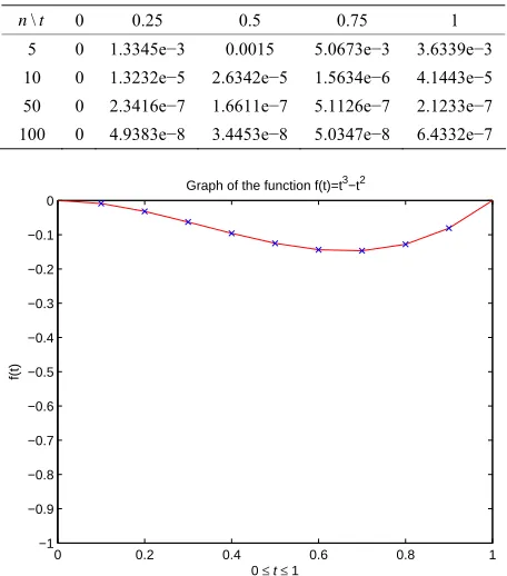
See Table 1 and Figure 1, where the exact solution is

 

₌ 3

y t t t and = , =3 1

2 2

  .

Example 4.1.2

 

 

 















 

















 



2

2

2 2

1

3 3

= 2

3 3 2

4 4

6

4 4 6

k

D y t D y t y t

t t

k _t

k _t

t

 

  

with the initial condition y

 

0 = 0,y

 

0 = 0 Hence

 

₌

_



1



_

_



1



_

2

1 1

i i i i i

x x k x

i i

i

x

  



     

   

 

     

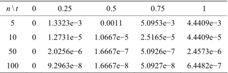
See Table 2 and Figure 2, where the exact solution is

 

₌ 2 3

y t t t and = , = 13

2

[image:4.595.309.537.221.480.2]

  .

Table 1. Absolute error of numerical solution of Example 4.1.

\

n t 0 0.25 0.5 0.75 1

5 0 1.3345e−3 0.0015 5.0673e−3 3.6339e−3 10 0 1.3232e−5 2.6342e−5 1.5634e−6 4.1443e−5 50 0 2.3416e−7 1.6611e−7 5.1126e−7 2.1233e−7 100 0 4.9383e−8 3.4453e−8 5.0347e−8 6.4332e−7

0 0.2 0.4 0.6 0.8 1

−1 −0.9 −0.8 −0.7 −0.6 −0.5 −0.4 −0.3 −0.2 −0.1 0

0 ≤ t ≤ 1

f(t)

[image:4.595.314.534.519.704.2]

Graph of the function f(t)=t3−t2

Figure 1. Numerical and analytic graph of solution of Ex- ample 4.1.

t 

 

 

 

 

 



 

      

 _  _

 _     _





     

  _      __

(20)

0 0.2 0.4 0.6 0.8 1

0 0.1 0.2 0.3 0.4 0.5 0.6 0.7 0.8 0.9 1

0 ≤ t ≤ 1

f(t)

Graph of the function f(t)=t2−t3

[image:5.595.60.286.111.184.2]

Table 2. Absolute error of numerical solution of Example 4.2.

\

n t 0 0.25 0.5 0.75 1

5 0 1.3323e−3 0.0011 5.0953e−3 4.4409e−3 10 0 1.2731e−5 1.0667e−5 2.5165e−5 4.4409e−5 50 0 2.0256e−6 1.6667e−7 5.0926e−7 2.4573e−6 100 0 9.2963e−8 1.6667e−8 5.0927e−8 6.4482e−7

5. Conclusion

From above, we imposed the Lane-Emden differential equation of fractional order. The generality of definition of Lane-Emden as a fractional order is more importance in applied mathematics, mathematical physics and astro- physics. The order appeared in two different fractional powers. An approximate solution is obtained by employ- ing the method of power series. Furthermore, a numerical solution is established by Collection method for these equations.

REFERENCES

[1] M. Yigider, “The Numerical Method for Solving Differ-ential Equations of Lane-Emden Type by Pade Approxi-mation,” Discrete Dynamics in Nature and Society, Vol. 2011, 2011, Article ID: 479396.

doi:10.1155/2011/479396

[2] R. P. Agarwal D. O. Regan and V. Lakshmikanthamr, “Quadratic Forms and Nonlinear Non-Resonant Singular Second Order Boundary Value Problems of Limit Circle Type,” Zeitschrift fur Analysis und ihre Anwendungen, Vol. 20, 2001, pp. 727-737.

[3] R. P. Agarwal and D. O. Regan, “Existence Theory for Single and Multiple Solutions to Singular Positone Boun- dary Value Problems,” Journal of Differential Equations, Vol. 175, No. 2, 2001, pp. 393-414.

doi:10.1006/jdeq.2001.3975

[4] R. P. Agarwal and D. O. Regan, “Existence Theory for Singular Initial and Boundary Value Problems: A Fixed Point Approach,” Applicable Analysis: An International Journal, Vol. 81, No. 2, 2002, pp. 391-434.

doi:10.1080/0003681021000022023

[5] M. M. Coclite and G. Palmieri, “On a Singular Nonlinear Dirichlet Problem,” Communications in Partial Differen-tial Equations, Vol. 14, No. 10, 1989, pp. 1315-1327. doi:10.1080/03605308908820656

[6] J. H. Lane, “On the Theoretical Temperature of the Sun under the Hypothesis of a Gaseous Mass Maintaining Its Volume by Its Internal Heat and Depending on the Laws of Gases Known to Terrestrial Experiment,” The Ameri-can Journal of Science and Arts, Vol. 50, 1870, pp. 57- 74.

[7] R. Emden, “Gaskugeln,” Teubner, Leipzig and Berlin, 1907.

[8] S. Chandrasekharr, “Introduction to the Study of Stellar Structure,” Dover, New York, 1967.

[9] M. Chowdhury and I. Hashim, “Solutions of Emden Fow- ler Equations by Homotopy-Perturbation Method,” Non- linear Analysis: Real World Applications, Vol. 10, No. 1, 2009, pp. 104-115. doi:10.1016/j.nonrwa.2007.08.017 [10] A. Yildirim and T. Öziş, “Solutions of Singular IVPs of

Lane-Emden Type by the Variational Iteration Method,” Nonlinear Analysis: Theory, Methods & Applications, Vol. 70, No. 6, 2009, pp. 2480-2484.

doi:10.1016/j.na.2008.03.012

[11] K. Parand and A. Pirkhedri, “Sinc-Collocation Method for Solving Astrophysics Equations,” New Astronomy, Vol. 15, No. 6, 2010, pp. 533-537.

doi:10.1016/j.newast.2010.01.001

[12] E. Momoniat and C. Harley, “An Implicit Series Solution for a Boundary Value Problem Modelling a Thermal Ex-plosion,” Mathematical and Computer Modelling, Vol. 53, No. 1-2, 2011, pp. 249-260.

doi:10.1016/j.mcm.2010.08.013

[13] K. Parand, M. Dehghan, A. Rezaeia and S. Ghaderi, “An Approximation Algorithm for the Solution of the Nonlin-ear Lane-Emden Type Equations Arising in Astrophysics Using Hermite Functions Collocation Method,” Com-puter Physics Communications, Vol. 181, No. 6, 2010, pp. 1096-1108. doi:10.1016/j.cpc.2010.02.018

[14] H. Adibi and A. Rismani, “On Using a Modified Legen-dre-Spectral Method for Solving Singular IVPs of Lane- Emden Type,” Computers & Mathematics with Applica-tions, Vol. 60, No. 7, 2010, pp. 2126-2130.

doi:10.1016/j.camwa.2010.07.056

[15] A. H. Bhrawy and A. S. Alofi, “A JacobiGauss Colloca-tion Method for Solving Nonlinear LaneEmden Type Equations,” Communications in Nonlinear Science and Numerical Simulation, Vol. 17, No. 1, 2012, pp. 62-70. [16] R. P. Agarwal and D. O. Reganr, “Singular Boundary

Value Problems for Superlinear Second Order Ordinary and Delay Differential Equations,” Journal of Differential Equations, Vol. 130, No. 2, 1996, pp. 333-335.

doi:10.1006/jdeq.1996.0147

[17] R. Lewandowski and B. Chorazyczewski, “Identification of the Parameters of the KelvinVoigt and the Maxwell Fractional Models, Used to Modeling of Viscoelastic Dampers,” Computers and Structures, Vol. 88, No. 1-2, 2010, pp. 1-17. doi:10.1016/j.compstruc.2009.09.001 [18] F. Yu, “Integrable Coupling System of Fractional Soliton

Equation Hierarchy,” Physics Letters A, Vol. 373, No. 41, 2009, pp. 3730-3733. doi:10.1016/j.physleta.2009.08.017 [19] K. Diethelm and N. Ford, “Analysis of Fractional Differ-ential Equations,” Journal of Mathematical Analysis and Applications, Vol. 265, No. 2, 2002, pp. 229-248. doi:10.1006/jmaa.2000.7194

[20] R. W. Ibrahim and S. Momanir, “On the Existence and Uniqueness of Solutions of a Class of Fractional Differ-ential Equations,” Journal of Mathematical Analysis and Applications, Vol. 334, No. 1, 2007, pp. 1-10.

doi:10.1016/j.jmaa.2006.12.036

Mathe-matical Analysis and Applications, Vol. 339, No. 2, 2008, pp. 1210-1219. doi:10.1016/j.jmaa.2007.08.001

[22] B. Bonilla, M. Rivero and J. J. Trujillor, “On Systems of Linear Fractional Differential Equations with Constant Coefficients,” Applied Mathematics and Computation, Vol. 187, No. 1, 2007, pp. 68-78.

doi:10.1016/j.amc.2006.08.104

[23] I. Podlubny, “Fractional Differential Equations,” Acade- mic Press, London, 1999.

[24] S. Zhangr, “The Existence of a Positive Solution for a Nonlinear Fractional Differential Equation,” Journal of Mathematical Analysis and Applications, Vol. 252, No. 2,

2000, pp. 804-812. doi:10.1006/jmaa.2000.7123

[25] R. W. Ibrahim and M. Darusr, “Subordination and Su-perordination for Analytic Functions Involving Fractional Integral Operator,” Complex Variables and Elliptic Equa-tions, Vol. 53, No. 11, 2008, pp. 1021-1031.

doi:10.1080/17476930802429131