Munich Personal RePEc Archive
Cherry Picking with Synthetic Controls
Ferman, Bruno and Pinto, Cristine and Possebom, Vitor
Sao Paulo School of Economics - FGV, Sao Paulo School of
Economics - FGV, Yale
11 March 2018
Cherry Picking with Synthetic Controls
∗Bruno Ferman† Cristine Pinto‡ Vitor Possebom§
Sao Paulo School of Economics - FGV Sao Paulo School of Economics - FGV Yale University
First Draft: June 2016 This Draft: March 2018
Please click here for the most recent version
Abstract
We evaluate whether a lack of guidance on how to choose the matching variables used in the Synthetic Control (SC) estimator creates specification-searching opportunities. We first provide theoretical results showing that specification-searching opportunities would be asymptotically ir-relevant when the number of pre-treatment periods goes to infinity when we restrict to a subset of SC specifications. However, based on Monte Carlo simulations and simulations with real datasets, we show significant room for specification searching when the number of pre-treatment periods is finite and when alternative specifications commonly used in SC applications are also considered. This undermines one of the potential advantages of the method, which is providing a transparent way of choosing comparison units and, therefore, being less susceptible to specification searching than alternative methods. To address this problem, we provide recommendations to limit the possibilities for specification searching in the SC method. Finally, we analyze the possibilities for specification searching and our recommendations in two empirical applications.
Keywords: inference; synthetic control; p-hacking; specification searching
JEL Codes: C12; C21; C33
∗We would like to thank Sergio Firpo, Ricardo Masini, Masayuki Sawada, and participants at the Sao School of
Economics seminar, Yale Econometrics Lunch, African Meeting of the Econometric Society, and the 2016 Meeting of the Brazilian Econometric Society for the excellent comments and suggestions. Deivis Angeli provided outstanding research assistance.
†Corresponding Author: (email) [email protected], (tel) +55 11 3799-3350, (fax) + 55 11 3799-3357
1
Introduction
The synthetic control (SC) method has been recently proposed in a series of seminal papers
byAbadie & Gardeazabal (2003),Abadie et al.(2010), and Abadie et al.(2015) as an alternative
method to estimate treatment effects in comparative case studies. Despite being relatively new,
this method has been used in a wide range of applications, including the evaluation of the impact
of terrorism, civil wars and political risk, natural resources and disasters, international finance,
education and research policy, health policy, economic and trade liberalization, political reforms,
labor, taxation, crime, social connections, and local development.1 Athey & Imbens(2017) describe
the SC method as arguably the most important innovation in the policy evaluation literature in
the last fifteen years.
Abadie et al. (2010) and Abadie et al. (2015) describe many advantages of the SC estimator
over techniques traditionally used in comparative studies. Among them, one important feature
of the SC method is that it provides a transparent way to choose comparison units. In the SC
method, a data-driven process is used to choose the weights that will build the weighted-average
of the controls’ outcomes that will represent the counterfactual for the treated unit. Also, since
the estimation of the SC weights does not require access to post-intervention outcomes, researchers
could decide on the study design without knowing how those decisions would affect the conclusions
of their studies. Taken together, these features potentially make the SC method less susceptible to
specification searching relative to alternative methods for comparative case studies. This could be
an important advantage of the SC method given the growing debate about transparency in social
science research (e.g.,Miguel et al. (2014)).2
An important limitation of the SC method, however, is that it does not provide clear guidance
1
SC has been used in the evaluation of the impact of terrorism, civil wars and political risk (Abadie & Gardeazabal
(2003),Bove et al.(2014),Li(2012),Montalvo(2011),Yu & Wang(2013)), natural resources and disasters (Barone & Mocetti(2014),Cavallo et al.(2013),Coffman & Noy(2011),DuPont & Noy(2012),Mideksa(2013),Sills et al.
(2015),Smith (2015)), international finance (Jinjarak et al.(2013), Sanso-Navarro(2011)), education and research
policy (Belot & Vandenberghe (2014), Chan et al. (2014), Hinrichs (2012)), health policy (Bauhoff (2014), Kreif
et al.(2015)), economic and trade liberalization (Billmeier & Nannicini(2013),Gathani et al.(2013),Hosny(2012)),
political reforms (Billmeier & Nannicini(2009),Carrasco et al.(2014),Dhungana(2011)Ribeiro et al.(2013)), labor
(Bohn et al. (2014), Calderon (2014)), taxation (Kleven et al. (2013), de Souza (2014)), crime (Pinotti (2012b),
Pinotti(2012a),Robbins et al.(2017),Saunders et al.(2014)), social connections (Acemoglu et al.(2013)), and local
development (Ando(2015),Gobillon & Magnac(2016),Kirkpatrick & Bennear(2014),Liu(2015),Possebom(2017),
Severnini(2014)).
2
on the choice of predictor variables and covariates that should be used to estimate the SC weights.3
Although Abadie et al. (2010) define vectors of linear combinations of pre-intervention outcomes
that could be used as predictors, there is no specific recommendation about which variables should
be used. Such lack of guidance on how to choose the predictors when implementing the synthetic
control method translates into a wide variety of different specifications in empirical applications of
this method. For example, some applied papers use all pre-treatment outcome lags as economic
predictors, other papers select a subset of the pre-treatment outcome lags as economic predictors,
while other papers use the mean of all pre-treatment outcome lags and other covariates as economic
predictors.4 If different specifications result in widely different choices of the SC unit, then a
researcher would have relevant opportunities to select “statistically significant” specifications even
when there is no effect.5 Since a researcher would usually not be able to commit to a particular
specification before knowing how these decisions would affect the conclusion of her study, this
flexibility may undermine one of the main advantages of the SC method.6
In this paper, we evaluate the extent to which this variety of options in the synthetic control
method creates opportunities for specification searching considering only one particular step of
the method: the choice of predictors used in the estimation of the SC weights.7 We first provide
3
To the best of our knowledge,Dube & Zipperer(2015) andKaul et al.(2015) are the only other authors to point
out that there is little explicit guidance in the SC literature to determine the choice of predictors. However, they do not explore the implications of such lack of specific guidance on the possibilities for specification searching in SC applications.
4
For example, Abadie & Gardeazabal(2003), Abadie et al. (2015) andKleven et al.(2013) use the mean of all
pre-treatment outcome values and other covariates as predictors;Billmeier & Nannicini (2013),Bohn et al.(2014),
Gobillon & Magnac(2016),Hinrichs(2012) use all the pre-treatment outcome values;Smith(2015) selects 4 out of
10 pre-treatment periods;Abadie et al. (2010) select 3 out of 19 pre-treatment periods; andMontalvo(2011) uses
only the last two pre-treatment outcome values.
5
We consider for inference the placebo test suggested in Abadie et al. (2010). Although this is not a formal
randomization test if treatment is not randomly assigned, we focus on this test because it is the most commonly used
test in SC application. FollowingAbadie et al.(2010), we can think of this test as the probability of having a test
statistic on the top 5% of the distribution of test statistics in the placebo runs. In practice, this is how most applied researchers evaluate whether the SC estimator is significant in their applications. Moreover, the randomization inference assumptions are valid in the data generating processes in our simulations. Therefore, the placebo test
is statistically valid in our simulations. SeeFirpo & Possebom (2017), Ferman & Pinto (2017) and Hahn & Shi
(2016) for details on the statistical properties of this test. As a robustness check, we also consider inference with an
infeasibletest in our MC simulations where we take advantage that the data generating process is known to calculate the distribution of the test statistics, instead of using the distribution of placebo runs as in the test proposed in
Abadie et al.(2010). All results are qualitatively the same.
6
Olken (2015) andCoffman & Niederle(2015) evaluate the use of pre-analysis plans in social sciences. For ran-domized control trials (RCT), the American Economic Association (AEA) launched a site to register experimental designs. However, there is no site where one would be able to register a prospective synthetic control study. More-over, in many synthetic control applications both pre- and post-intervention information would be available to the researcher before the possibility of registering the study. In this case, it would be unfeasible to commit to a particular specification.
7
conditions under which different SC specifications lead to asymptotically equivalent estimators when
the number of pre-treatment periods (T0) goes to infinity, as long as we restrict to specifications
such that the number of pre-treatment outcome lags used as predictors goes to infinity withT0.8
Under these conditions, we also show that the placebo test suggested inAbadie et al. (2010) will
asymptotically lead to the same conclusion, as long as we restrict to this subset of SC specifications.
However, these results leave open the possibility for specification searching in SC applications for at
least two reasons. First, many SC applications do not have a large number of pre-treatment periods
to justify large-T0 asymptotics, as argued in Doudchenko & Imbens(2016), which may still leave
room to specification searching even if we restrict to this class of SC specifications. Moreover, there
are common SC specifications that do not satisfy the condition on the number of pre-treatment
periods used as predictors going to infinity, which might lead to specification-searching opportunities
even when the number of pre-treatment periods is large.
Guided by our theoretical results, we then evaluate the extent to which specification searching
may be a problem in SC applications using Monte Carlo (MC) simulations and placebo simulations
with the Current Population Survey (CPS). We calculate the probability that a researcher would
find at least one specification such that the ratio of post/pre mean squared prediction error (MSPE)
of the actual intervention is in the top 5% distribution of the post/pre MSPE estimated for units
not exposed to the intervention when the actual effect of the intervention is zero, which would
lead him/her to interpret the results as “significant”. If different SC specifications lead to similar
SC estimators, then this probability would be close to 5%, while it may be much higher than 5%
if different SC specifications lead to wildly different estimates, implying that there is room for
specification searching. We consider six different specifications commonly used in SC applications:
(1) all pre-treatment outcome values, (2) the first three quarters of the pre-treatment outcome
values, (3) the first half of the pre-treatment outcome values, (4) odd pre-treatment outcome
values, (5) even pre-treatment outcome, (6) the mean of all pre-treatment outcome values, and (7)
the researcher. For example,Kl¨obner et al.(2016) show that different SC estimators are obtained depending on the
software used or on how the dataset is sorted.
8
three outcome values (the first, the middle and the last ones).9,10 We focus on the placebo test suggested inAbadie et al.(2010) to assess the “statistical significance” of the estimates because this
is how researchers usually assess whether their results are significant in SC applications. While, as
noticed inAbadie et al.(2010), this is not generally a formal statistical test when treatment is not
randomly assigned, it is still informative about whether or not the estimated effect of the actual
intervention is large relative to the distribution of the effects estimated for units not exposed to the
intervention. Importantly, note that the conditions such that this test is actually valid are satisfied
in our simulations. Moreover, we also consider as a robustness check an infeasible test based on
actual distribution of the test statistic in our MC simulations to assess the statistical significance
of the results, and we find similar results. Therefore, our results are not driven by potential size
distortions of the placebo test. For brevity, we refer to this probability of having an extreme test
statistic in the placebo test as the probability of rejecting the null throughout the paper.
We find that the probability of detecting a false positive in at least one specification for a 5%
significance test can be as high as 14% when there are 12 pre-treatment periods (25% if we consider
a 10% significance test). The possibilities for specification searching remain high even when the
number of pre-treatment periods is large. For example, with 400 pre-treatment periods, we still
find a probability of around 13% that at least one specification is significant at 5% (24% if we
consider a 10% significance test). These results suggest that, even with a large number of
pre-treatment periods, different specifications can still lead to significantly different synthetic control
units, generating substantial opportunities for specification searching. This is true both in data
generating processes with stationary and non-stationary common factors. We also find similar
results in placebo simulations using the CPS. Importantly, we still find that the probability of
rejecting the null in at least one specification can be significantly higher than the nominal test size
even when we restrict the set of choices to specifications with a good pre-treatment fit.11
9
In order to simplify the presentation of our results, we do not consider in our simulations the use of time-invariant
covariates, as is commonly used in specifications that rely on the pre-treatment outcome mean. In AppendixBwe show
that our results remain valid if we consider specifications that use time-invariant covariates as economic predictors in addition to functions of the pre-treatment outcomes. Note also that these seven specifications do not exhaust all specification options that have been considered in SC applications.
10
Note that specifications (1)-(5) satisfy the condition in our theoretical results that the number of pre-intervention
periods used as predictor variables increase withT0.
11
There are at least two possible explanations for still finding over-rejection even when we condition on specifications
with a good pre-treatment fit. First, in many SC applications, including those inAbadie & Gardeazabal (2003),
Given our theoretical results, it is expected that the significant specification-searching
possibil-ities with a largeT0 are driven by specifications that do not increase the number of pre-treatment
lags used as predictors when the number of pre-treatment periods goes to infinity. Indeed, we find
that excluding the specifications whose number of pre-intervention periods used as predictor
vari-ables do not increase withT0 from the set of options strongly attenuates the specification-searching
problem whenT0 is large, although we still find room for specification searching when T0 is not so
large. Note that the data-generating process (DGP) in our MC simulations also provides a way
to measure the extent to which different specifications assign positive weight to control units that
should not be considered in the synthetic control unit. Consistent with the intuition that
specifica-tions that use more pre-treatment outcome lags as predictors would better control for unobserved
confounders, we find that the specifications that limit the number of pre-treatment outcome lags
misallocate substantially more weights, suggesting that such specifications should not be considered
in SC applications.
It is important to note that our results by no means imply that researchers that have
imple-mented the SC method did engage in specification searching. Given that this is a relatively new
method, there would not be enough papers to formally test for specification searching.12 However,
given the mounting evidence that there is a high return for reporting “significant” results and that
scientists tend to engage in p-hacking, our findings raise important concerns about the synthetic
control method.13 Also, while we find room for specification searching in the SC method, it does
not imply that this problem is more relevant for the SC method when compared to alternatives
trend, as shown inFerman & Pinto (2016). Our results suggest that, in this scenario, different SC specifications
can still yield substantially different estimators even if most specifications provide a good approximation to the
non-stationary trend. Second, as shown inFerman & Pinto(2017), the SC permutation test can lead to over-rejection if
we consider the SC estimator conditional on a good pre-treatment fit. This explains why we may still have significant over-rejection even when the researcher has only a few (or even just one) specifications with a good pre-intervention fit to choose from.
12
Brodeur et al.(2016) analyzes 641 articles (providing more than 50,000 tests) published in theAmerican Economic Review, theJournal of Political Economy, and theQuarterly Journal of Economics. They identify a residual in the
distribution of tests that cannot be explained solely by journals favoring rejection of the null hypothesis.Simonsohn
et al.(2014) suggest the use of the p-curve as a way to distinguish between selective reporting findings and true effects. One of the requirements to the inference from p-curve to be valid is that we have a great pool of studies from which we can select studies and p-values that test similar hypothesis. Given that the synthetic control estimator is a relatively recent method, there would not be enough published papers that used this method even if we consider a wide range of journals. Therefore, it would be unfeasible to replicate these methodologies for synthetic control applications.
13
methods.14 The main conclusion of our paper is that, despite providing a data-driven method
to construct the counterfactual unit, the SC method does not completely solve the
specification-searching problem due to a lack of consensus on how the SC weights should be estimated.
If there were a consensus on how the SC specification should be selected, then the risk of
p-hacking (at least in this dimension) would be limited. Our results suggest that restricting the
set of options for researchers can strongly attenuate this problem, particularly if we restrict to
specifications that use many pre-treatment outcome lags as predictors. Another possible solution
would be to require researchers applying the SC method to report results for different specifications.
However, it is important to note that testing all the possible SC specifications separately would
not provide a valid hypothesis test since there would not be a defined decision rule (see White
(2000)). One alternative is to consider a test statistic for the permutation test that combines the
test statistics for all individual specifications, as suggested inImbens & Rubin(2015).
Finally, we also consider the possibilities for specification searching and the implementability
of the above recommendations in two empirical applications, based on Smith (2015) and Abadie
et al. (2010). In our empirical examples, we analyze three cases: one whose conclusion is robust
to specification searching, one where different specifications can reach either significant and
non-significant results (clearly showing the potential for specification searching in the synthetic control
framework), and one where all results are significant, but at different significance levels. Moreover,
after applying our recommendations, we show that one can reach a clear conclusion about the
significance of the results in all three examples.
The remainder of this paper proceeds as follows. In Section 2, we provide a brief overview of
the SC estimation, and then we derive conditions under which the SC estimators using different
specifications will be asymptotically equivalent when the number of pre-treatment periods goes to
infinity. Then, we provide Monte Carlo simulations in Section 3 and simulations with real data
in Section 4. We present our main recommendations in Section 5, and we discuss three empirical
examples in Section6. We conclude in Section7.
14
For example,Gardeazabal & Vega-Bayo(2016) compare the synthetic control method with a panel data approach
2
Synthetic Control Method and Specification Searching
Abadie & Gardeazabal(2003),Abadie et al.(2010) andAbadie et al.(2015) have developed the
Synthetic Control Method in order to address counterfactual questions involving only one treated
unit and a few control units. Intuitively, this method estimates the potential outcome of the
treated unit if there were no treatment by constructing a weighted average of control units that
is as similar as possible to the treated unit regarding the pre-treatment outcome variables and
covariates. For this reason, this weighted average of control units is known as the synthetic control
unit and treatment effects can be flexibly estimated for each post-treatment period. Below, we
followAbadie et al. (2010), explaining their estimator.
Suppose that we observe data for (J+ 1) ∈Nunits during T ∈N time periods. Additionally,
assume that there is a treatment that affects only unit 1 from periodT0+ 1 to periodT
uninter-ruptedly, whereT0∈(1, T)∩N. Let the scalarYj,t0 be the potential outcome that would be observed for unit j in period t if there were no treatment for j ∈ {1, ..., J + 1} and t ∈ {1, ..., T}. Let the
scalarY1
j,t be the potential outcome that would be observed for unit j in periodtif unitj received
the treatment from periodT0+ 1 toT. Define:
αj,t :=Yj,t1 −Yj,t0 (1)
as the treatment effect for unitj in period tand Dj,t as a dummy variable that assumes value 1 if
unitj is treated in period tand value 0 otherwise. With this notation, we have that the observed
outcome for unitj in periodtis given by
Yj,t :=Yj,t0 (1−Dj,t) +Yj,t1Dj,t.
Since only the first unit receives the treatment from periodT0+ 1 toT, we have that:
Dj,t:=
1 ifj= 1 and t > T0
0 otherwise.
We aim to identify (α1,T0+1, ..., α1,T). SinceY 1
Let Yj := [Yj,1...Yj,T0]
′
be the vector of observed outcomes for unit j ∈ {1, ..., J + 1} in the
pre-treatment period andXja (F×1)-vector of predictors ofYj. Those predictors can be not only
covariates that explain the outcome variable, but also linear combinations of the variables inYj.15
Let alsoY0 = [Y2...YJ+1] be a (T0×J)-matrix andX0= [X2...XJ+1] be a (F×J)-matrix.
Given the choice of predictors in matrix Xj, the idea of the SC method is to construct the
counterfactual for the treated unit using a weighted average of the control units:
b
Y10,t :=
J+1
X
j=2
b
wjYj,t (2)
The weightsWc = [wb2...wbj+1]′ :=Wc(Vb)∈RJare given by the solution to a nested minimization problem:
c
W(V) := arg min
W∈W(X1−X0W) ′V(X
1−X0W) (3)
where W := nW= [w2...wJ+1]′ ∈RJ :wj ≥0 for eachj∈ {2, ..., J + 1} and PJj=2+1wj = 1
o
and
Vis a diagonal positive semidefinite matrix of dimension (F×F) whose trace equals one. Moreover,
b
V:= arg min
V∈V(Y1−Y0Wc(V)) ′(Y
1−Y0Wc(V)) (4)
whereV is the set of diagonal positive semidefinite matrix of dimension (F×F) whose trace equals
one.
Finally, we define the Synthetic Control Estimator ofα1,t (or the estimated gap) as
b
α1,t :=Y1,t−Yb1N,t (5)
for eacht∈ {1, ..., T}.
Intuitively, Wc is a weighting vector that measures the relative importance of each unit in the
synthetic control of unit 1 andVb measures the relative importance of each one of theF predictors.
Abadie et al. (2010) discuss alternative ways to choose the matrix Vb. We focus our attention on
15
For example, if the outcome variable is a country’s per capita GDP andT0= 12,Xjmay contain the investment
the most common method of choosingVb, which involves solving the nested minimization problem
given by equations (3) and (4).
Even though a crucial part in the implementation of the SC method is the choice of economic
predictors, there is little guidance about which variables should be included in matrix Xj. This
lack of guidance can create an opportunity for the researcher to look for specifications that yield
“better” results by including or excluding some pre-treatment outcome values from its specification.
This risk is even greater when we consider that there is no consensus about which functions of the
outcome values should be included inXj: Abadie & Gardeazabal (2003),Abadie et al.(2015) and
Kleven et al. (2013) use the mean of all pre-treatment outcome values and additional covariates;
Smith(2015) uses Yj,T0,Yj,T0−2, Yj,T0−4 and Yj,T0−6; Abadie et al. (2010) picks Yj,T0,Yj,T0−8 and
Yj,T0−13; Billmeier & Nannicini (2013), Bohn et al. (2014), Gobillon & Magnac (2016), Hinrichs (2012) use all pre-treatment outcome values; and Montalvo (2011) uses only the last two
pre-treatment outcome values.16
A key question, therefore, is whether different specifications may lead to substantially different
SC estimators. We consider the asymptotic behavior of different SC specifications whenT0 → ∞.
We define a specifications by the set of predictorsXj(s, T0) that are used when there areT0 pre-treatment periods. Let I(s, T0) be the set of pre-treatment periods t such that Yj,t is included as
a predictor when there areT0 pre-treatment periods, and let L(s, T0) = #I(s, T0).17 Let y0−j,t be
theJ×1 vector of potential outcomes for all units except unitjat time t. We consider a sufficient
assumption to guarantee that a broad set of SC specifications will be asymptotically equivalent
whenT0→ ∞.
Assumption 1 For any sequence of integers{tk}k∈Nwithtk> tk−1, and for anyj∈ {1, ..., J+ 1},
we have that:
sup W∈W
1
K
K
X
k=1
Yj,t0k−y−j,t0 k′W2−Qj(W)
p
→0 whenK → ∞ (6)
whereQj(W) is a continuous and strictly convex function.
16
By no means we imply that those authors have engaged in specification searching. We have only listed them as prominent examples of different choices regarding predictor variables.
17
For example, let a specificationsbe such thatR covariates and the first half of the pre-treatment outcome lags
are used as predictors. ThenI(s, T0) ={1,2, ...,T02 }andL(s, T0) = T02 . Note that, in this case, the dimension ofXj
would beR+T0
Note that assumption 1 implies that pre-treatment averages of the second moments of every
subsequence of (Y10,t, ..., YJ0+1,t) converge to the same value. We show in Appendix A that this assumption is satisfied if, for example, we assume that {y0
ty0t ′
}T0
t=1 is weakly stationarity, each element of {y0
ty0t ′
} has absolutely summable covariances, and Ehy0
ty0t ′i
is non-singular, where
y0
t = (Y10,t, ..., YJ0+1,t)′.
Given these assumptions, we have the following results:18
Proposition 1 Let Wc(s, T0) be the SC weights using specification s when there are T0
pre-intervention periods. If L(s, T0) → ∞ when T0 → ∞, then, under assumption 1, Wc(s, T0)
p
→
W=argminW∈WQ1(W).
Corollary 2 Let ˆα1t(s, T0) and ˆα1t(s′, T0) be two SC estimators for the treatment effect at time
t > T0 using specifications s and s′ such that L(s, T0) → ∞ and L(s′, T0) → ∞ when T0 → ∞. Then, under assumption1,|αˆ1t(s, T0)−αˆ1t(s′, T0)|=op(1).
Therefore, while different SC specifications may generate different SC estimates, our result
from Proposition1 and Corollary2 show that, under some conditions, different specifications will
lead to asymptotically equivalent SC estimators, as long as the number of pre-treatment lags used
as predictors goes to infinity with T0. Note, however, that our results do not guarantee that
different SC specifications would lead to similar SC estimates when T0 is finite. Moreover, there
are common specifications used in SC applications that do not satisfy the condition on the number
of pre-treatment lags used as economic predictors going to infinity with T0. For example, many
authors consider the use of the mean of all pre-treatment outcome values in addition to other
covariates as economic predictors, while other authors consider the use of only a few pre-treatment
outcome lags as economic predictors. These alternative specifications would generally lead to SC
weights that will not converge toW, so there may still be significant variation in the SC estimates
even whenT0 is large.
Note that our results are valid irrespectively of whether the SC estimator is unbiased, as we are
only comparing the asymptotic behavior of the SC estimator under different specifications. For a
thorough analysis on the asymptotic bias of the SC estimator whenT0 → ∞, see Ferman & Pinto 18
(2016). In our simulations in Sections3and4, the condition in which the SC estimator is unbiased
are satisfied. Also, note that our results are related to the results fromKaul et al.(2015), who show
that covariates would become irrelevant in the minimization problem3if all pre-treatment lags are
included as predictors. Since our result from Proposition1 holds whether or not we include other
covariates as predictors, this implies that covariates would also become asymptotically irrelevant
in the minimization problem3 whenever we consider specifications such that L(s, T0)→ ∞ when
T0 → ∞, even if we do not include all pre-treatment outcome lags. Note, however, that this does
not necessarily imply that the SC weights will not attempt to match the covariates of the treated
unit nor that the SC estimator will be asymptotically biased, as explained inBotosaru & Ferman
(2017).
Conditional on a given SC specification, Abadie et al. (2015) propose an inference procedure
that consists in a straightforward placebo test. They permute which unit is assumed to be treated
and estimate, for each j ∈ {2, ..., J + 1} and t ∈ {1, ..., T}, αbj,t as described above. Then, they
compute the test statistic
RM SP Ej :=
PT t=T0 +1
Yj,t−Ydj,tN 2
/(T−T0) PT0
t=1
Yj,t−Ydj,tN 2
/T0
where the acronym RMSPE stands forratio of the mean squared prediction errors. Moreover, they
propose to calculate a p-value
p:=
PJ+1
j=1 1[RM SP Ej ≥RM SP E1]
J+ 1 , (7)
where1[⋄] is the indicator function of event⋄, and reject the null hypothesis of no effect if pis less
than some pre-specified significance level, such as the traditional value of 0.05. Abadie et al.(2010)
recognize that the randomization inference assumptions are very restrictive for the SC set-up, as
treatment is not, in general, randomly assigned.19 In the absence of random assignment, they
interpret the p-value as the probability of obtaining an estimate value for the test statistics at least
as large as the value obtained using the treated case as if the intervention was randomly assigned
19
Firpo & Possebom (2017) discuss a sensitivity mechanism analysis for this test, while Ferman & Pinto(2017)
analyze the statistical properties of this placebo test when treatment is not randomly assigned. Hahn & Shi(2016)
also consider the properties of placebo test in the SC setting. For our purposes in this paper, we considerAbadie
among the data. Although the p-value from this placebo test lacks a clear statistical interpretation,
this test is commonly used in SC application. Therefore, our simulation exercises can be seen as
the probability that a researcher applying the SC method would find a test statistic that is in the
top 5% of the distribution of test statistics in the placebo runs, which is how researchers applying
the SC method usually assess whether their estimates are significant. Moreover, note that, in our
simulations, the placebo test considering a single SC specification would have a rejection rate under
the null of 5% by construction.
As a corollary from Proposition 1, we show that the ranking of RM SP Ej will remain
asymp-totically invariant to changes in the SC specification when T0 → ∞ as long as we consider only
specifications such that the number of pre-treatment outcome lags goes to infinity withT0.
Corollary 3 Under assumption1and assuming thatYjtis continuous, the ordering of{RM SP E1, ...,
RM SP EJ+1} is asymptotically invariant to SC specifications such that L(s, T0) → ∞ when
T0 → ∞and T −T0 is finite.
The result from corollary 3shows that, if we restrain to SC specifications such that number of
pre-treatment outcome lags goes to infinity withT0, then the possibilities for specification searching
would be limited, as a test based on different SC specifications would lead to the same conclusion
with probability approaching to one when T0 → ∞. It is important to emphasize, however, that
we may still have room for specification searching ifT0 is finite. Moreover, this result is not valid if
we consider alternative SC specifications such that the number of pre-treatment outcome lags used
as economic predictors remain fixed whenT0→ ∞.
3
Monte Carlo Simulations
In the previous section, we provide theoretical results showing that possibilities for specifications
searching should be limited if a researcher restraints herself to specifications that uses an infinitely
large number of pre-intervention outcome values asT0 → ∞. Therefore, proposition1and
corollar-ies2 and3 provide guidance on the conditions in which specification searching could be a relevant
problem in SC applications: (i) whenT0 is not large and/or (ii) when one considers specifications
on such guidance.
In the Monte Carlo exercise, we generate 10,000 data sets and, for each one of them, test
the null hypothesis of no effect whatsoever adopting several different specifications. Conditional
on a given specification, in our simulations this placebo test should provide a rejection rate of
α% under the null for a α% significance test by construction. We are interested, however, in the
probability of rejecting the null hypothesis at the 5%-significance level for at least one specification.
If different specifications result in wildly different SC estimators, then the probability of finding one
specification that rejects the null atα% can be significantly higher thanα%. In the extreme case in
which we haveKdifferent specifications and these specifications lead to independent estimators, this
probability would be given by 1−(1−α)K, whereK is the number of different specifications.20 In this case, such lack of guidance about which specifications should be used could generate substantial
opportunities for specification searching. In contrast, if different SC specifications lead to similar
SC weights, then this rejection rate will be close to α% and the risk of specification searching
would be very low. We consider two data generating processes. In Section 4, we consider placebo
simulations with the CPS.
In the first data generating process (DGP), we consider a linear factor model in which all units
are divided into groups that follow different stationary time trends.
Yj,t0 =δt+λkt +ǫj,t (8)
for some k = 1, ..., K. We consider the case in which J + 1 = 20 and K = 10. Therefore, units
1 and 2 follow the trendλ1t, units 3 and 4 follow the trend λ2t, and so on. We consider that λkt is normally distributed following an AR(1) process with 0.5 serial correlation parameter,δt∼N(0,1)
andǫj,t ∼N(0,0.1).
In our second DGP, we modify the linear factor model such that a subset of the common factors
are non-stationary. In this case, we consider DGP which includes a non-stationary trend φr t that
follows a random walk:
Yj,t0 =δt+λtk+φrt+ǫjt (9)
20
for some k = 1, ..., K and r = 1, ..., R. We consider in our simulations K = 10 and R = 2.
Therefore, unitsj = 2, ...,10 follow the same non-stationary pathφ1t as the treated unit, although only unitj= 2 also follows the same stationary path λ1
t as the treated unit.
In both models, we impose that there is no treatment effect, i.e., Yj,t = Yj,t0 = Yj,t1 for each
time periodt∈ {1, ..., T0}. We fix the number of post-treatment periodsT −T0= 10 and we vary
the number of pre-intervention periods in the DGPs,T0 ∈ {12,32,100,400}. In the Appendix, we
consider variations in our stationary model (8) by setting (i) ǫj,t ∼ N(0,1), (ii) K = 2, or (iii)
including time-invariant covariates. We find similar results as the ones presented in the main text.
We calculate the SC estimator using the following seven specifications that differ only in the
linear combinations of pre-treatment outcome values used as predictors:21
1. All pre-treatment outcome values: Xj = [Yj,1· · ·Yj,T0]′
2. The first three fourths of the pre-treatment outcome values: Xj =
Yj,1· · ·Yj,3T0/4
′
3. The first half of the pre-treatment outcome values: Xj =Yj,1· · ·Yj,T0/2
′
4. Odd pre-treatment outcome values: Xj =Yj,1 Yj,3· · ·Yj,(T0−3) Yj,(T0−1)
′
5. Even pre-treatment outcome values: Xj =
Yj,2 Yj,4· · ·Yj,(T0−2) Yj,T0
′
6. Pre-treatment outcome mean: Xj = [PTt=10 Yj,t/T0]
7. Three outcome values (the first one, the middle one, and the last one): Xj =Yj,1 Yj,T0/2 Yj,T0
′
Observe that specifications 1-5 satisfy the conditions of Proposition1and Corollaries2and3, while
specifications 6 and 7 do not. We stress that, in order to simplify the presentation of our results,
we do not consider in our MC simulations the use of time-invariant covariates, as is commonly
used in specifications that rely on the pre-treatment outcome mean. In AppendixBwe show that
our results remain valid if we consider specifications that use time-invariant covariates as economic
predictors in addition to functions of the pre-treatment outcomes.
21
In order to compute the SC estimator, we use theSynthpackage inR. (SeeAbadie et al.(2011) for details.) This
package solves the nested minimization problem described by equations (3) and (4). We specify the optimization
method to be BFGS only and use optimization routine Low Rank Quadratic Programming when Interior Point
For each specification, we run a placebo test using the RMSPE test statistic proposed inAbadie
et al.(2010) and reject the null at 5%-significance level if the treated unit has the largest RMSPE
among the 20 units. By construction, this leads to a 5% rejection rate when we look at each
specification separately. We are interested, however, in the probability that we would reject the
null at the 5%-significance level in at least one specification. This is the probability that a researcher
would be able to report a significant result even when there is no effect if she were to engage in
specification searching. If all different specifications result in the same synthetic control unit, then
we would find that the probability of rejecting the null in at least one specification would be equal
to 5% as well. However, this probability may be higher if the synthetic control weights depend on
specification choices, which may be the case in finite samples or for specifications 6 and 7.
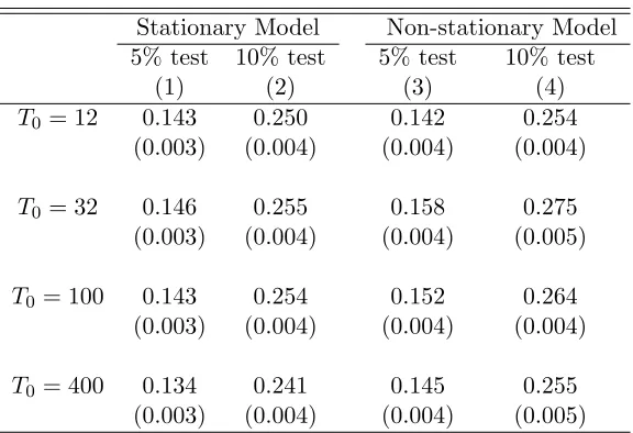
We present in columns 1 and 2 of Table 1 the probability of rejecting the null at 5% and
at 10% significance levels in at least one of our seven specifications for the stationary model.
Columns 3 and 4 present the same results for the non-stationary model.22 With T
0 = 12, a
researcher considering these seven different specifications would be able to report a specification
with statistically significant results at the 5% level with probability 14.3% for the stationary model
and 14.2% for the non-stationary. If we consider 10% significance tests, then the probability of
rejecting the null in at least one specification would be up to 25.0% and 25.4%, respectively for the
stationary and the non-stationary models. Therefore, with few pre-treatment periods, a researcher
would have substantial opportunities to select statistically significant specifications even when the
null hypothesis is true. Importantly, note that it is not unusual to have SC applications with as
few as 12 pre-intervention periods.23
If the variation in the SC weights across different specifications vanishes when the number of
pre-treatment periods goes to infinity even for the specifications that do not satisfy the assumption
of Proposition1 and Corollaries 2 and 3, then we would expect the rejection rate to get closer to
5% once the number of pre-treatment periods gets large. In this case, all different specifications
would provide roughly the same SC unit and, therefore, the same treatment effect estimate. The
results in Table1show that the probabilities of rejecting the null are still significantly higher than
22
See tableA.1for results using different data generating processes.
23
See, for example, Abadie & Gardeazabal(2003), Kleven et al.(2013), Kreif et al. (2015), Smith(2015), Ando
(2015),Liu(2015),Sills et al.(2015),Billmeier & Nannicini(2013),Bohn et al.(2014),Cavallo et al.(2013),Hinrichs
the test size even when the number of intervention periods is large. In a scenario with 400
pre-intervention periods, in the non-stationary model it would be possible to reject the null in at least
one specification 14.5% (25.5%) of the time for a 5% (10%) significance test.24 These results suggest
that, when we include specifications that violate the conditions of Proposition 1 and Corollaries
2 and 3, specification searching remains a problem for the SC method even when the number of
pre-intervention periods is remarkably large for empirical applications.
In the previous exercise, we assumed that the researcher would be able to choose any of the 7
specifications we considered in our MC simulations. However,Abadie et al.(2010) andAbadie et al.
(2015) emphasize that the SC control estimator should only be used in the situations with good
pre-treatment fit, i.e., in situations in which the weighted average of the controls’ pre-treatment
outcomes is a good approximation for the treated pre-treatment outcome. It is important, therefore,
to check whether the specification-searching problem we identified in the SC method arises because
we allow the researcher to choose specifications that provide a poor pre-treatment fit. We consider
a pre-treatment normalized mean squared error index to determine whether a specification provides
a good pre-treatment fit:25
˜
R2 = 1−
PT0
t=1
Y1,t−Yb1N,t
2
PT0
t=1 Y1,t−Y1
2 (10)
whereY1 =
PT0
t=1Y1,t
T0 . If this measure is one, then we have a perfect fit. 26
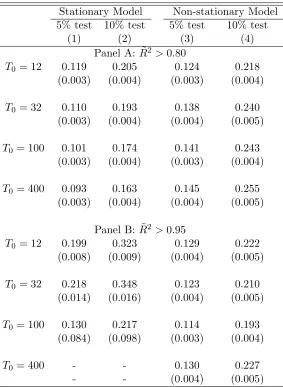
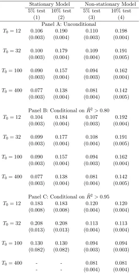
In order to capture a good fit, we consider two thresholds for ˜R2, ˜R2 > 0.80 and ˜R2 > 0.95.
Considering these two thresholds, panel A of Table2 shows the probability of finding a good
pre-treatment fit for at least one of the seven specifications. The probability of finding specifications
24
Note that the probability of specification searching is not monotonic inT0. This happens because, with a very
smallT0, the chance that a pre-treatment MSPE is close to zero is very high. Since there is a high correlation of
pre-treatment MSPE across specifications, it is likely that one unit will have a pre-treatment MSPE close to zero for many specifications. This implies that this unit will have a large test statistic for all these specifications, so the
placebo test will reject the null for these specifications most of the time. AsT0increases, the probability of having a
pre-treatment MSPE close to zero will be small.
25
This measure is very similar to the “pre-treatment fit index” proposed byAdhikari & Alm(2016). These authors
propose a measure that is the ratio between the squared root of the mean squared predicted error (the numerator
of 1−R˜2
) and
rPT
0
t=1Y1t2
T0 . The advantage of our measure relative to the one proposed byAdhikari & Alm(2016)
is that our measure is invariant to linearly additive changes. Dube & Zipperer(2015) also propose a pre-treatment
fit criterion that is equal to the numerator of our measure, the root of the mean squared error predictor between the synthetic and the actual outcomes in the pre-treatment period. However, differently from our suggestion, their measure is not scale invariant.
26
with a good pre-treatment fit depends crucially on how we define whether a specification provided a
good fit and on whether we consider a stationary or a non-stationary model. We present in columns
1 and 2 the results for the stationary model. With a moderateT0, the probability of finding at least
one specification with good fit is close to one when we consider the weaker definition of good fit,
and close to zero when we consider the more stringent definition. We highlight that, according to
panels B and C, the specifications that do not satisfy the conditions of Proposition1and Corollaries
2and 3 have a relatively small chance of providing a good pre-intervention even under the weaker
definition of good fit, illustrating that this kind of specification behaves poorly in small samples.
We present, in columns 3 and 4, the results for the non-stationary model. In this case, the
probability of having at least one specification with a good fit is close to one even when we consider
the more stringent definition of good fit. Also, there is a high probability that all specifications
(including specifications 6 and 7) provide a good fit, especially when T0 is large. This happens
because, with large T0, the non-stationary factors dominate the variance of Y1,t. Since the SC
estimator is extremely efficient in controlling for the non-stationary factors (seeFerman & Pinto
(2016)), it will usually provide a good pre-treatment fit.
Given these definitions of good fit, we present in Table 3 the probabilities of rejecting the
null in at least one specification when we restrict the researcher to consider only specifications
that provide a good pre-treatment fit. Note that the possibilities for specification searching in
the non-stationary model (columns 3 and 4) are virtually the same as when we do not restrict for
specifications with a good pre-treatment fit, especially whenT0is large (columns 3 and 4 of Table1).
This is not surprising, given that all specifications will usually provide a good pre-treatment fit in
this model. For the stationary model (columns 1 and 2 of Table3), the specification-search problem
is attenuated when we restrict to specifications with a good fit if we use the more lenient definition
of good fit (panel A). In practice, in this case the restriction of considering only specifications
with a good fit prevents the researcher from choosing specifications 6 and 7, whose weights, as we
show below, are very different from the ones chosen by the other specifications, that satisfy the
conditions of the conditions of Proposition 1 and Corollaries 2 and 3. If we consider the more
stringent definition of good fit, however, then the probability of rejecting the null in at least one
specifications is substantially higher (panel B). This happens because, if we consider that the SC
(2010) and Abadie et al. (2015)), then there is a low probability of finding a good fit for at least
one specification and we would only consider specifications such that the denominator of the test
statistic for the treated unit is close to zero. Since the test statistic for the placebo units are not
conditional on a good pre-treatment, this leads to over-rejection, as shown in Ferman & Pinto
(2017).
Overall, these results suggest that restricting the researcher to consider only specifications with
a good fit does not necessarily attenuate the specification-searching problem. On the one hand, if
conditioning on a good fit does not actually restrict the set of options a researcher has (as happens
with our non-stationary model), then we have the same results as in the unconditional case. On
the other hand, if conditioning severely restricts the set of options, then we have over-rejection
because the test statistic for the treated unit is conditional on a denominator that is close to zero,
while the test statistics for the placebo units are unconditional.
The results so far indicate that different specifications can provide substantially different SC
estimators in finite samples. However, based on our theoretical results from section 2,
specifica-tions 1-5 should provide similar SC weights, while specificaspecifica-tions 6-7, that lie outside the scope of
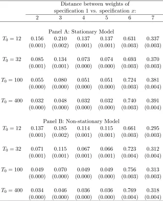
Proposition1, could potentially provide SC weights that differ wildly. To analyze this possibility,
we calculate a measure of variability of weights in comparison to specification 1. For each
specifi-cationx∈ {2, ...,7}, we compute the difference between the weight allocated by specification 1 and
specificationxfor each unit in the donor pool. Then, we take the maximum value of this difference
across units in the donor pool. We present this measure for specifications 2-7 on table 4. On the
one hand, analyzing specifications 2-5, we find that the variability of weights between specifications
is small and, most importantly, decreasing when the pre-intervention period gets large, as expected
given our theoretical results. On the other hand, for specifications 6 and 7, we find strikingly
differ-ent results: their weights differ substantially from the weights of specification 1 and this difference
does not decrease when the pre-intervention period gets large.
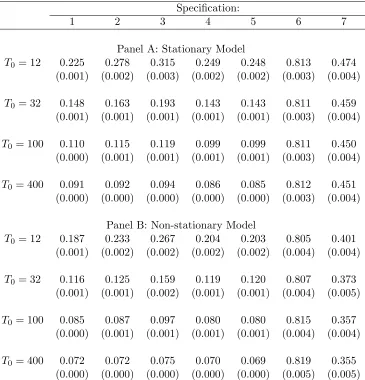
Beyond the variability of weights between specifications, an interesting feature of our MC
simu-lations is that the SC estimator should assigned positive weights only for unit 2 (which has the same
factor loadings of unit 1), so we can actually calculate the proportion of weights that is
misallo-cated for each specification. We present in columns 1 to 7 of Table5the proportion of misallocated
do not satisfy the conditions of proposition 1, misallocate substantially more weights relative to
the other specifications. In particularly, specification 6, which uses the pre-treatment mean as
eco-nomic predictor, does a particularly poor job. For the stationary model (panel A), with T0 = 12,
specifications 6 and 7 misallocates more than 80% and 45% of the weights, while the misallocations
for other specifications ranges from 23% to 32%. Most importantly, the misallocation of weights
decreases withT0 for all specifications, except for specifications 6 and 7. Results are qualitatively
the same for the non-stationary model (panel B). These results suggests that specifications outside
the scope of proposition1, such as specification 6 and 7, behave poorly because they do not capture
the time-series dynamics of the units, which is the main goal of the SC method.27,28
Given that specifications 6 and 7 stand out by misallocating significantly more weights and
by picking weights that are very different from the ones chosen by specification 1, we consider, in
Table6, the specification-searching possibilities excluding specifications 6 and 7. As expected based
on corollary 3, excluding specifications 6 and 7 significantly attenuates the specification-searching
problem, especially when the number of pre-treatment periods is large.29 However, it does not
completely solve the problem even whenT0 is moderate. Importantly, although corollary3suggests
that specification-searching possibilities within a well defined class of specifications should be very
small asymptotically, we still find room for specification-searching even whenT0 is relatively large
in comparison to usual dataset sizes in common SC applications.
We also stress that the attenuation in the specification-searching problem after excluding the
specifications outside the scope of corollary3is not simply because we are considering five
specifi-cations instead of seven. If we exclude, for example, specifispecifi-cations 2 and 3 instead of specifispecifi-cations
6 and 7, then there is virtually no change in the specification-search problem relative to the case
that we consider all seven specifications (Appendix TableA.2).
27
Although any specification could potentially take into account the time series dynamics of the outcome variable
because the matrixV is chosen to minimize the pre-treatment MSPE in the second step of the optimization process,
this process is very limited because the first minimization problem can severely restrict the set of possible weights
W∗(V) that may be chosen in the second step, as suggested inFerman & Pinto(2016).
28
In Appendix B, we show that specifications 6 and 7 can fail to properly exploit the time-series dynamics of the
data even if we also include time-invariant covariates as economic predictors. In this case, they will still remain different from the specifications that use many pre-treatment outcome lags as economic predictors. Therefore, our result that the possibilities of specification searching may not diminish with the number of pre-treatment periods
when we consider specifications outside the scope of proposition1remains valid even if we consider the addition of
time-invariant variables as economic predictors.
29
The only exception is when we consider the stationary model conditional on a good fit with ˜R2 >0.95. This
Finally, as a robustness check, we take advantage of the fact that the DGP is known in our MC
simulations, and we replicate our results using an infeasible test based on the actual distributions
of the test statistics to determine whether the SC estimator for a given specification is statistically
significant. The results based on this infeasible test, presented in Appendix TableA.4, corroborate
the results presented in this section, showing that our results are not driven by distortions of the
placebo test used in the SC inference.
4
Simulations with Real Data
The results presented in Section 3 suggest that different specifications of the SC method can
generate significant specification-searching opportunities in finite samples. In particular, we also
find that using only specifications that satisfy the conditions of proposition1and corollaries 2and
3 alleviate this problem even though it does not solve it completely. We now check whether the
results we find in our MC simulations are also relevant when we consider real datasets by conducting
simulations of placebo interventions with the Current Population Survey (CPS). We use the CPS
Merged Outgoing Rotation Groups for the years 1979 to 2014. Following Bertrand et al. (2004),
we extract information on employment status and earnings for women between ages 25 and 50. We
also consider in a separate set of simulations information on men in the same age range.
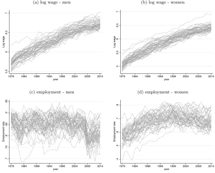
Before we proceed to the placebo simulations, we briefly discuss the raw data for these outcome
variables. There are important distinctions in the time series characteristics when we consider
information for men versus women and when we consider log wages versus employment. Figures1a
and1b present the time series of log wages for all US states, respectively for men and women. As
expected, the time series of log wages is non-stationary and increasing for both men and women.
These graphs suggest that there is a strong non-stationary factor that affects all states in the same
way. Figures 1c and 1d present the time series of employment for all US states, respectively for
men and women. In this case, the time series for men should be closer to our stationary model
from Section 3, while the time series for women has an increasing trend in the 80s and 90s.
We first consider simulations with 12 pre-intervention periods, 4 post-intervention periods, and
20 states. In each simulation, we randomly select one treated and 19 control states out of the 51
1999. Then we consider simulations with 32 pre-intervention periods, 4 post-intervention periods,
and 20 states. In this case, we randomly select 20 states and use the entire 36 years of data. In
each scenario, we run 5,000 simulations using either employment or log wages as the dependent
variable and test the null hypothesis using the same seven specifications of Section3.30
We start presenting the probability of finding specifications with a good fit in Table 7. When
the outcome variable is log wages, the probability of having at least one specification with a good
fit is close to one, especially when we considerT0 = 32 (columns 1 to 4, panel A). Most importantly,
when we considerT0 = 32, specifications 6 and 7 have a high probability of fitting the data closely.
These results are consistent with our MC simulations considering that the log wages series appear
to have important non-stationary common factors. The probability of finding specifications with a
good fit is lower when we consider employment instead of log wages as outcome variable, and even
lower when we consider men relative to women. This is consistent with the employment time series
for men being closer to a stationary process.
We present in Table 8 the probabilities of rejecting the null in at least one specification.31 In
panel A, we present the specification-search probabilities including any of the seven specification
that provide a good fit, i.e., ˜R2 > 0.80. The results are very similar to our findings in the MC
simulations. WithT0 = 12, depending on the sample and outcome variable, there is 13-26%
proba-bility of finding a specification with statistically significant results at 5% and a 21-41% probaproba-bility
of finding a specification with statistically significant results at 10%. With T0 = 32 these
proba-bilities are slightly lower, but still significantly higher than the test nominal size for all cases but
men employment rates. In panel B, we present the results searching only specifications that satisfy
the conditions of corollary 3, i.e., we exclude specifications 6 and 7. As in our MC simulations,
restricting to specifications 1-5 reduce the specification-searching problem but do not solve it
en-tirely. In particularly, for T0 = 32, we cannot reject the null hypothesis that the rejection rate is
equal to the nominal level for all but one case. We stress that this reduction is not a mechanical
consequence of searching five instead of seven specification. If we exclude specifications 2 and 3, we
find rejection rates that are very similar to the ones including all seven specifications.32 In general,
30
Standard errors are clustered at the level of the treated state when we calculate the probability of having a good fit and when we calculate rejection rates.
31
Standard errors for these simulation results are clustered at the treated-state level, in order to take into account that the simulations are not independent.
32
these results suggest that specification-searching possibilities in SC applications can be relevant
in real applications of the SC method even when we restrict ourselves to specifications that have
satisfy the conditions of proposition1and corollaries 2and 3.
5
Recommendations
The specification-searching problem we identify arises from a lack of consensus about which
specifications should be used in SC applications. Our first recommendation is that researchers
should only consider specifications that satisfy the conditions of proposition1and corollaries2and
3— i.e., specifications that uses an infinitely large number of pre-intervention outcome values when
the pre-intervention period gets large — because our results suggest that the specification-searching
problem is magnified by specifications with undesirable properties, such as the specification that
uses only the mean pre-treatment outcome as economic predictor or the one that uses only the
initial, middle and final pre-intervention outcome values. If we discard these specifications, then the
specification-searching problem is attenuated, especially if we have a large number of pre-treatment
periods, even though it does not solve the problem completely.
We also recommend that researchers applying the SC should report results for different
spec-ifications. However, even if a researcher present results for all possible SC specifications with an
hypothesis test for each specification, this would not provide a valid hypothesis test. If the decision
rule is to reject the null if the test rejects in all specifications, then we could end up with a very
conservative test (Romano & Wolf (2005)).33 If the decision rule is to reject the null if the test
rejects in at least one specification, then we would be back in the situation where we over-reject
the null. One possible solution is to base the inference procedure on a new test statistic that is
a function that combines all the test statistics for the individual specifications, as suggested by
Imbens & Rubin(2015).The drawback of this solution is that it does not provide an obvious
point-estimator. There are two possible ways to handle this disadvantage. First, if the test function is
simply a weighted average of the test statistics for individual specifications, then Christensen &
Miguel(2016) andCohen-Cole et al.(2009) suggest using the same weights to compute a weighted
33
When we adopt this decision rule in our MC simulations, then probability of rejecting the null at 5% for all specifications is lower than 1% in all scenarios. If we discard specifications 6 and 7, then this rejection rate ranges
average of the point-estimator of each specification and using this weighted average as an estimate
that incorporates model uncertainty. As another alternative, we can focus on set identification, as
suggested byFirpo & Possebom(2017). In this case, we would invert this combination of test
statis-tics to compute confidence sets that contain all treatment effects functions within a pre-specified
class that are not rejected by the inference procedure that uses the chosen combination of test
statistics.
6
Empirical Applications
We analyze the possibilities for specification searching and the implementability of our
recom-mendations in two empirical examples.
6.1 The resource curse exorcised: Evidence from a panel of countries (Smith
(2015))
Smith (2015) evaluates the impact of major natural resource discoveries since 1950 on GDP
per capita using different methods, including the synthetic control method.34 Major oil and gas
discoveries happened in Equatorial Guine and Ecuador in 1992 and 1972 respectively, implying that
pre and post-treatment periods are 1950-1991 and 1992-2008 for the first country and 1950-1971
and 1972-2008 for the second one. While the donor pool for Equatorial Guine consists of
Sub-Saharan African Countries (Benin, Burkina Faso, Burundi, Cameroon, Cape Verde, Central African
Republic, Chad, Cote d’Ivoire, Gambia, Ghana, Guinea, Kenya, Lesotho, Liberia, Madagascar,
Malawi, Mali, Mauritania, Mauritius, Mozambique, Namibia, Niger, Rwanda, Senegal, Somalia,
Sudan, Swaziland, Tanzania, Togo, Uganda, Zambia, Zimbabwe), the donor pool for Ecuador
consists of Latin American and Caribbean countries (Costa Rica, Cuba, Dominican Republic, El
Salvador, Guatemala, Honduras, Jamaica, Nicaragua, Panama, Paraguay, Puerto Rico, Uruguay).
We estimate the impact of major oil and gas discoveries on GDP per capita using the synthetic
control method with fourteen different specifications. Specifically, we test seven different
specifica-tions that differ in which funcspecifica-tions of the pre-treatment periods are included and, for each one of
34
Following the best practices in terms of transparency and replicability, he made his dataset and replication files
them, we either include two covariates35 or not. Our seven basic specifications are:36
1. All pre-treatment outcome values: Xj =Yj,(T0−6)· · ·Yj,T0
′
2. The first three fourths of the pre-treatment outcome values: Xj =
Yj,(T0−6)· · ·Yj,(T0−2)
′
3. The first half of the pre-treatment outcome values: Xj =Yj,(T0−6)· · ·Yj,(T0−4)
′
4. Odd pre-treatment outcome values: Xj =Yj,(T0−5) Yj,(T0−3) Yj,(T0−1)
′
5. Even pre-treatment outcome values (Original Specification ): Xj =
Yj,(T0−6) Yj,(T0−4) Yj,(T0−2) Yj,T0
′
6. Pre-treatment outcome mean: Xj = [PTt=T00 −6Yj,t/7]
7. Three outcome values: Xj =Yj,(T0−6) Yj,(T0−3) Yj,(T0)
′
whereT0 = 1991 for Equatorial Guine andT0 = 1971 for Ecuador.
Table 9 shows the p-value and our goodness of fit measure for each specification and each
country. On the one hand, the results for Equatorial Guinea are robust to specification searching,
since all specifications provide treatment effect estimates that are significant at the 5%-level. On
the other hand, the results for Ecuador show that the researcher could try different specifications
and pick one whose result is significant. In particular, all fourteen specifications have a good fit
( ˜R2 > 0.80), but only two of them are significant (specifications 4b and 6b), implying that the
researcher could, potentially, report a false-positive result.37
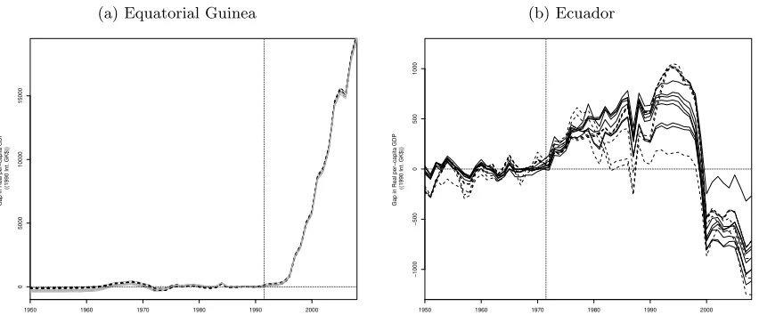
We now test our recommendations in these particular applications. First of all, by presenting
results for more than one specification as we do in Table 9, a sensible conclusion would be that
major oil and gas discoveries had a significant effect on Equatorial Guinea’s GDP per capita even
though there is no evidence of such effect on Ecuador’s GDP per capital. Figure 2 shows that
35
The included covariates are ethnic fragmentation and population size one year before the discovery.
36
Although the number of pre-treatment years is larger than seven, we followed Smith(2015) and considered for
this exercise different specifications using only seven years of pre-treatment data in the first minimization problem
(equation (3)) while accounting for the entire pre-treatment period in the second minimization problem (equation
(4)). Had we considered only seven years of pre-treatment data in the second step, we would reach similar conclusions
to the ones in the main text. Had we considered the same specifications using the full pre-treatment data in the first step, then we would fail to reject the null for all specifications. This is consistent with our result that the variation between specifications that use pre-treatment outcome lags as economic predictor diminishes when the number of pre-treatment periods increases. Results are available upon request.
37
We stress that the specification considered bySmith(2015) is not one of these three that would have led him to
this conclusion is reasonable since, in the case of Equatorial Guinea, we find that all specifications
with a good fit have estimates of similar magnitude while, in the case of Ecuador, our results vary
widely across specifications. The next step is to test the null hypothesis using a test statistics that
combine the test statistics of all specifications. Restricting ourselves to specifications with good
fit ( ˜R2 > 0.80), we find that the p-value of a test that uses the mean of the RMSPE statistic
across specifications, as suggested by Imbens & Rubin (2015), is equal to 0.031 and 0.308 for
Equatorial Guinea and Ecuador, corroborating our conclusion that the treatment effect is positive
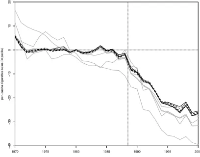
in the first case and zero in the second one. Now, following the suggestion of Christensen &
Miguel (2016) and Cohen-Cole et al. (2009), figure 3 shows the average treatment effect across
specifications with good fit as a black line and the associated placebo effects as gray lines. Clearly,
the effects for Equatorial Guinea and Ecuador are, respectively, large and small when compared to
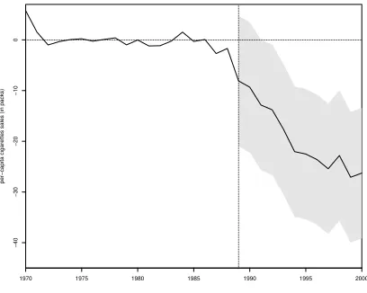
their empirical distributions. Finally, in line with the suggestions ofFirpo & Possebom (2017), we
invert tests based on the mean of the RMSPE statistic across specifications to compute confidence
sets for the treatment effect over time. Our confidence sets (see figure 4) include all treatment
effect functions that we fail to reject using this combined test statistic, considering functions that
are deviations from the average treatment effect across specifications by an additive and constant
factor. Analyzing sub-figure4a, we see that, although we cannot reject treatment effect functions
that are initially negative, all treatment effect functions in our confidence sets increase very fast,
becoming positive after a few years of treatment. For Ecuador (see sub-figure4b), we find that our
confidence set include a zero effect for almost all years after the beginning of treatment, suggesting
that the discovery of oil and gas in Ecuador had almost no impact on per-capita GDP.
For Equatorial Guinea and Ecuador, the results based on the recommendations by Imbens &
Rubin(2015),Christensen & Miguel(2016),Cohen-Cole et al.(2009) andFirpo & Possebom(2017)
point all to the same direction. Therefore, a reasonable conclusion would be that the treatment
effect is significant for Equatorial Guinea and not significant for Ecuador.
6.2 Synthetic Control Methods for Comparative Case Studies: Estimating the
Effect of California’s Tobacco Control Program (Abadie et al. (2010))