206
Encoder-decoder models for latent phonological representations of words
Cassandra L. Jacobs
University of California, Davis [email protected]
Fr´ed´eric Mailhot
Autodesk Inc.
Abstract
We use sequence-to-sequence networks trained on sequential phonetic encoding tasks to construct compositional phonological representations of words. We show that the output of an encoder network can predict the phonetic durations of American English words better than a number of alternative forms. We also show that the model’s learned representations map onto existing measures of words’ phonological structure (phonolog-ical neighborhood density and phonotactic probability).
1 Introduction
The representation of linguistic categories is a fun-damental problem in (psycho)linguistics and nat-ural language processing. The formation of com-plex representations from more basic components is relevant at all levels of linguistic representa-tion, semantic, syntactic, and phonological. Find-ing good representations for words’ phonological1 structure is critical in psycholinguistics, where we wish to understand the phonological structure of the lexicon, which has been shown to be relevant for language comprehension and production.
The distributional hypothesis defines a word by the context in which it occurs (Harris,1954;Firth,
1957). This approach has been extended more re-cently to other types of compositional structures, for example in characterizing the meanings and forms of sentences (Cer et al.,2018;Joulin et al.,
2017;Conneau et al., 2017;Devlin et al., 2018). In this paper we explore whether distributional ap-proaches can capture important phonological de-pendencies.
1
There are disagreements in the literature about the lo-cation (Hale and Reiss, 2008) and even existence (Ohala, 1990b) of the boundary/interface between phonetics and phonology, so we remain as theory-agnostic as pos-sible, freely using “phonological”/“phonetic” and “seg-ment”/“phone” interchangeably.
Specifically, we test the extent to which recur-rent encoder-decoder models (Cho et al., 2014;
Sutskever et al., 2014) can learn representations that characterize the phonological structure of the lexicon while also having linguistic and psycho-logical validity (Sibley et al., 2008). We pro-pose that this approach can be used to learn viable lexical-level phonological representations. The output of the encoder component of our model yields promising results in the prediction of pho-netic duration, outperforming a number of alter-nate phonological representations of words.
2 Quantifying a word’s phonology
Given a set of discrete phonetic symbols i.e. graphemes with conventionalized pronunciations such as the International Phonetic Alphabet, it is trivial to represent any word’s pronunciation as a sequence of such symbols. Conversely, relating sequences of such symbols (viz. words) to each other, as well as to the entire lexicon is less obvi-ous. This challenge has led to a proliferation of measurements that characterize a word’s phonetic or phonological relationship with all other words in the lexicon. We summarize some salient exam-ples below, and briefly discuss some of their short-comings.
2.1 Metrics insensitive to serial order
Phonological neighborhood density (PND). This measure is defined as the number of words having a Levenshtein edit distance of one from a given word (in terms of phonetic or phonologi-cal symbols) (Luce and Pisoni,1998;Levenshtein,
1966). Under this definition, a word like “cat” has many neighbors, while a word like “molt” has fewer. This measure is simple to calculate and a wide variety of resources exist for obtaining these measures across many languages (Marian et al.,
While conceptually simple, PND is insensitive to the position of a segment within a word (e.g. word-initial versus word-final substitutions), and so “sat” and “cab” are treated as equally similar to “cat”. Additionally, identifying a word’s phono-logical neighbors using the Levenshtein distance metric requires specifying how many sounds can be added, deleted, or substituted, and potentially the allowable edit distance2, increasing the num-ber of choice points in determining what a “neigh-borhood” is.
Frequency-weighted phonological neighbor-hood density. An augmented version of PND, which weights phonological neighbors in pro-portion to their lexical frequencies (standardly estimated from large corpora; Marian et al.,
2012). So, a more common word like “hat” would contribute more to the neighborhood den-sity of “cat” than a less common word like “cap”, even though they are at equal string edit dis-tance. Whether and to what extent density mea-sures should be frequency-weighted is an empiri-cal question, though these measures seem to better reflect psycholinguistic processes than frequency-insensitive measures.
Feature-wise similarity. In the phonologi-cal literature it is standard to represent segments as collections of articulatory or acoustic features, e.g. [+voice], [-obstruent] (Chomsky(1968) is the canonical reference). Some linguists (e.g. Frisch
(1996), inter alia) have posited that words like “cat” and “cap”, which differ only in the place of articulation of their final segments (alveolar ver-sus labial), should be considered more similar than e.g. “cat” and “can”, which differ in both voicing and manner of articulation. This measure of simi-larity is potentially controversial, as there are the-oretical and empirical questions as to which tures to include, or even whether phonetic fea-tures exist at all (Stevens and Blumstein, 1981;
Marslen-Wilson and Warren,1994).
2.2 Metrics incorporating serial order
All of the previously described measures effec-tively characterize words as unordered collections of segments. These characterizations are incom-plete because they fail to capture the fact that words unfold over time in usage. Representing the positions of phones within a word is critical for
ex-2See e.g. Su´arez et al., 2011 who allow edit distance
greater than one, and track the mean distance to a fixed num-ber of neighbors
plaining a number of aspects of language process-ing. For example, the beginnings of words con-tribute more strongly than their ends to psycholin-guistic effects that are attributed to their phono-logical representations (Levelt et al.,1999;Sevald and Dell,1994, inter alia), and a word’s phono-logical similarity to the rest of the words in the lexicon has important consequences for speech comprehension (Buz and Jaeger, 2016; Metsala,
1997). Some computational models encode seg-ments as a function of their linear position within a syllable, e.g. in aonset-vowel-codaformat (e.g.
Dell, 1986; Sevald and Dell, 1994). Other ap-proaches include segment n-grams to encode local aspects of serial order (e.g. Seidenberg and Mc-Clelland,1989;Davis,2010) and the oft-lamented Wickelphone (Houghton and Hartley,1996). Most closely related to the present approach, some work has demonstrated the viability of sequence en-coder models for representing sequences of char-acters or phonetic segments (Sibley et al.,2008).
2.3 Incorporating variability into representations
Psycholinguistic measures that quantify words’ phonological properties in the lexicon generally ignore their variability in pronunciation. In usage, segmental context, or lexical factors such as word frequency, can significantly influence the phonetic realization of a given phone, ranging from assimi-latory processes (Ohala,1990a) to massive reduc-tion and even complete omission (Pitt et al.,2005;
Johnson,2004,inter alia). For example, there are over 200 distinct transcriptions of the word “and” in the Buckeye corpus (Pitt et al., 2005), and its normative, dictionary pronunciation (i.e. [ænd]) only accounts for 3% of its realizations.
Measures such as PND rely on single, fixed pronunciations (generally normative/dictionary-based) and corpus-derived lexical frequencies to estimate how many similar-sounding words a given word has, but take no account of variabil-ity in realization. As there is evidence that listen-ers remember and can access/use individual exem-plars of perceived speech (Pierrehumbert, 1980;
“and” may rarely compete during lexical access, given that “and” is rarely pronounced similarly to “sand.” By incorporating the variability available in naturalistic speech corpora, we hope to provide a better characterization of a word’s phonological properties and its relation to the lexicon.
3 Latent phonological representations
Representing arbitrary-length sequences of phones with a single distributed representation has a number of potential practical and conceptual advantages. On the practical side, these repre-sentations have a fixed dimensionality, so finding meaningful groupings or clusters is computa-tionally more tractable than directly clustering variable-length sequences. Moreover, projecting these sequences into a latent space offers the potential of discovering hidden relationships or variables that affect phonological or lexical structure.
Our aim in this paper is to test whether and to what extent recent approaches to building sentence representations can also be applied to the phono-logical domain. Both simpler and more complex latent representations can be constructed to char-acterize the phonological forms of words. We first discuss potential “na¨ıve” means of accomplishing this, and then move into discussion of our pro-posed model.
Principal components on bag-of-n-phones
A number of document classification schemes and information retrieval tasks have treated documents as a product of the vector representations of words learned by principal components analysis (PCA;
Landauer and Dumais, 1997). We apply this to the phonetic domain as well. By analogy to a bag of words, we refer to bag-of-phones (unigram features) and bag-of-n-phones (higher-order seg-ment co-occurrence categories), which can then be fed into a dimensionality reduction algorithm like principal components analysis (PCA) as an approximate composition function to produce la-tent phonological representations of words.
doc2vec
Another dimensionality reduction method extends the continuous bag-of-words algorithm used to learn word vectors (Mikolov et al., 2013) to the document domain. Specifically, the model learns to compose (predict) a document (i.e. a word) from its phonological contents. doc2vec (Le and
Mikolov,2014) has been used in information re-trieval and natural language processing applica-tions (Lau and Baldwin, 2016) and so may be a viable way to obtain lexical phonological repre-sentations. As with bag-of-phones, this model is insensitive to serial order.
Sequential representations
Encoder-decoder or sequence-to-sequence
(seq2seqhenceforth) neural network architectures have shown considerable success in encoding sentences (viz. sequences of words) for tasks such as machine translation (Sutskever et al.,
2014;Cho et al.,2014). These methods may be appropriate as a means of composing segmental representations, as they are intrinsically sensitive to ordering, easily take usage frequencies into account (directly from training corpora), and have been shown to be effective learners of sequential distributional properties of their training data.
4 Seq2seq model
We trained seq2seq models to either reproduce their input, or to recover (predict) normative (dic-tionary) pronunciations from the phonetic tran-scriptions of words in the Buckeye corpus (Pitt et al.,2005), a dataset of monologues provided in response to interviewer questions about the talk-ers’ hometown of Columbus, Ohio. The corpus contains approximately 300,000 words.
Data inclusion criteria. There are some tran-scription errors in the Buckeye corpus, and so we excluded combinations of phones that did not oc-cur at least ten times. This removes many errors, but a few remain. For example, the segment “h” occurs in some transcriptions but is not part of the character set of the transcription dictionary, and is thus likely an error of omission for actual digraphs from the dictionary; “th”, “hh”, etc. Despite the presence of these remaining errors, we do not cor-rect the transcriptions of any words. In total, 57 phone/segment categories are represented. Full documentation of the coding scheme used in the corpus can be read inPitt et al. (2005). For bag-of-n-phones features, we add the additional char-acters “w s” and “w e” as word boundary charac-ters, signaling the starts and ends of words, respec-tively.
There are no standard train/dev/test splits for the Buckeye corpus, and so we restricted ourselves to randomly selected 80/20 train/test split (Pitt et al.,
Figure 1: Encoder-decoder LSTM architecture (Nor-mative decoder; for the Observed decoder, the output is the observed phonetic sequence).
Model architecture. Methodologically, we ap-proach the problem with an eye to restricting the computational power of our model, and to re-stricting the space of hyperparameters to explore. To this end, our models use a basic recurrent encoder-decoder architecture, with an input-side embedding layer, and single-layer, unidirectional3 LSTMs (Hochreiter and Schmidhuber, 1997) on the encoder and decoder sides. The encoder takes as input a sequence of phone indices (e.g. “cat”
→ [’k’, ’ae’, ’tq’]→ [11, 1, 20]), em-beds them, and encodes the sequence in the space defined by the LSTM. The encoder LSTM’s final hidden state is provided as input to the decoder, whose task is to “unroll” this latent representa-tion. The outputs of the decoder LSTM are suc-cessively fed through a softmax, sequentially out-putting class probabilities for each character class in the phone vocabulary, which are then decoded via simpleargmax(see Figure1).
4.1 Training
Hyperparameters. The number of training epochs was empirically determined on the basis of asymptoting training loss, which we determined to be 25 epochs. We used a cross-entropy loss func-tion, using the Adam optimizer (Kingma and Ba,
2015) with a learning rate of 0.001. Other Adam parameters were at default values in the dynet
python implementation as of this writing (version 2.0.3; Neubig et al.,2017). All hyperparameters were selected on the basis of asymptoting loss on a small subset of the training set. The embedding
3While we do not perform these experiments here, we
be-lieve that a Bi-LSTM encoder (Schuster and Paliwal,1997) will enable further advances in constructing psycholinguisti-cally predictive word representations.
layer had 32 dimensions, and the encoder and de-coder LSTMs were 64-dimensional.
Tasks. We trained two models to perform slightly different decoding tasks; the Norma-tive Decoder model, and the Observed Decoder
model. In both tasks, the inputs are transcriptions of observed realizations of words in the Buck-eye corpus, which include e.g. phonetic changes and omissions. The Normative Decoder’s task is to output the word’s normative pronunciation (e.g. [k, ae, tq] → [k, ae, t]), while the Observed Decoder model is trained as a se-quential autoencoder (e.g. Chung et al., 2016); the task is to reproduce the input sequence exactly. Both are potentially viable approaches to the cre-ation of lexical phonological representcre-ations and show similar performance in the downstream tasks reported on below, which may be useful for re-searchers who only have access to normative pro-nunciations.
We evaluated the performance of the model on the 20% held-out portion of the corpus.
4.2 Lexical representations
Once the model is trained, any sequence of phones can be input to the encoder, yielding a latent phonological representation of that sequence. As with character-based NLP models, the compara-tively low dimensionality of the input space (57 segments) mitigates sparsity issues, consequently we can obtain latent phonological representations not just of vocabulary words that have been trained but also for rare, out-of-vocabulary (OOV) words and non-words. We plot some aspects of the learned representations in Figures 2 and 3. One pattern that is particularly apparent is that the left-to-right serial nature of the encoder leads to repre-sentations that strongly encode the final segment in their representations, for both consonants and vowels.
5 Evaluation
As a preliminary investigation of the informa-tion encoded in the learned lexical representainforma-tions, we assess their ability to model phonetic dura-tion, which is known to be sensitive to phono-tactic probability and phonological overlap (Gahl et al.,2012;Watson et al.,2015;Buz and Jaeger,
Figure 2: Topology of word vectors from phonological encoder models learned by t-SNE (Maaten and Hinton,
2008). Degree to which word vectors encode vowel information. Clusters largely prioritize word-final information, especially the last segment. Left graph represents the identities of the first segment. Right graph represents the identities of the final segment. The strong encoding of the final segment may be due to the model architecture using uni-directional recurrent layers.
Figure 3: Topology of word vectors, t-SNE projection (Maaten and Hinton,2008). Degree to which word vectors encode consonant information. Clusters largely prioritize word-final information, especially the last segment. Left graph represents the identities of the first segment. Right graph represents the identities of the final segment.
Cohen Priva and Jaeger, 2018; Seyfarth, 2014). We show that the encoder creates sequence repre-sentations that are useful for predicting word du-ration, and compare the success of the encoder to several other models, described below.
5.1 Predicting word duration
Ultimately we are interested in whether latent phonological representations have predictive va-lidity for phonetic cues, potentially in conjunc-tion with other phonological and lexical repre-sentations. Word duration has been shown to be strongly related to phonological structure (Gahl et al.,2012), because duration may reflect the me-chanics of the phonological sequencing process in language production (Yiu and Watson,2015; Wat-son et al.,2015;Fox et al.,2015) or because speak-ers lengthen words in dense neighborhoods to pro-mote the listener’s understanding (Tily and
Kuper-man,2012).
We built a series of nested statistical models de-signed to predict whole-word phonetic duration. The durations were obtained by summing up the durations of each of the annotated phonetic seg-ments for an individual word, which are them-selves derived from time stamps extracted from the Buckeye metadata. Whole-word durations were log transformed due to their positive skew; failing to account for this can make statistical in-ference more difficult (Campbell,1992). All mod-els were constructed using ridge (L1 norm) re-gression using the scikit-learn package in Python (version 0.2.0;Pedregosa et al.,2011). We report goodness of fit measures in all cases by
R2 values (the coefficient of determination; pro-vided automatically by thescore function within the ridge regression model object).
[image:5.595.98.503.294.439.2]80-20% split that was used to train the encoder-decoder. Consequently, there were 282,742 obser-vations (words) during training, and 70,686 words at test. The vocabulary for the bag-of-words rep-resentations was estimated from the training data. All models are summarized in Table1.
5.2 Baseline models
Word embeddings. A word’s distributional prop-erties, such as its part of speech and meaning; la-tent part-of-speech; or word-frequency informa-tion may reliably predict a word’s durainforma-tion ( Sey-farth, 2014; Turnbull et al., 2018; Priva, 2015). Consequently, we incorporate 100-dimensional word embeddings into the regression models. We obtained these word embeddings from gensim’s (Reh˚uˇrek and Sojkaˇ , 2010) skip-gram implemen-tation trained on the Fisher corpus (Cieri et al.,
2004), which we selected due to its size, which is critical for generating good word embeddings (Antoniak and Mimno,2018), and because it be-longs to the same domain as the Buckeye corpus (conversational speech).
The skip-gram model used a context window of 5 words and a negative sampling size of 5. We used a zero vector to represent OOV (e.g. Colum-bus, Ohio-specific place names that would not oc-cur in the Fisher corpus). Word embeddings were, on their own, not a strong predictor of word dura-tion (R2 = 0.082) on the test set, but nevertheless account for some of the variance in word duration. Bag-of-phones models. Bag-of-words repre-sentations are a useful and informative baseline in other NLP tasks, especially text classification (Wang and Manning,2012). We obtained bag-of-phone representations by learning a vocabulary on the training data and creating sparse count vectors in which the features represent individual phones. A simple bag-of-uniphones model, which ignores order information, has greater predictive power than word embeddings on the test set (R2=0.140). This shows that it is possible to at least partly pre-dict the duration of a given word’s realization from relatively unstructured phonological information.
Bag-of-n-phones. Unlike bag-of-words repre-sentations, bag-of-ngrams encode localized order information. We constructed n-gram features of phone combinations (bag-of-n-phones) of lengths 2 to 5, using a cutoff frequency of 10 observations. These more complex representations performed similarly to the simpler bag-of-phones model on
the test set (R2 =0.140).
We also tested whether incorporating word boundary information into these models (“w s” and “w e” phones) would induce boundary-sensitive phonotactics, but this also did not pro-vide additional gains over simpler models (R2 = 0.138 andR2= 0.140).
Principal components analysis over bag-of-n-phones. Following from the previous section, we take our bag-of-n-phones representations and feed them into a truncated singular value de-composition model to obtain latent representa-tions of words (“documents”). This representation explained a slightly greater amount of variance in word duration than word embeddings (R2 = 0.106). However, this method performed far worse than the bag-of-phones and bag-of-n-phones mod-els described in the previous section, indicating that some information is lost in this dimensionality reduction method.
doc2vec. Our doc2vec model vectors were trained to predict a word from a phonological rep-resentation. The resulting vectors had the same dimensionality as the PCA vectors and the en-coder output of the seq2seq models. Surprisingly, doc2vec performed the worst of models that we considered (R2= -0.05).
seq2seq. The outputs of the encoders for the Observed and Normative decoder models were among the best we considered, both on their own and in conjunction with other measures. Inter-estingly, theObserved Decoder provides a much closer fit to phonetic duration than word embed-dings, bag-of-phones, PCA, doc2vec, and the Nor-mative Decoderrepresentations. When combined with bag-of-phones and word embedding infor-mation, theObserved Decoderrepresentations ex-plain the greatest amount of variance in word du-ration (R2 = 0.181), suggesting that these latent phonological representations encode useful infor-mation for characterizing word form.
Simple TestR2 No. features Combined TestR2 No. features
Word embeddings (WE) 0.082 100 BoP + wb + WE 0.161 159
Bag-of-phones (BoP) 0.140 57 + Observed decoder 0.181 223
+ w s + w e (wb) 0.140 59 + Normative decoder 0.177 223
Bag-of-n-phones (BoNP) 0.140 1700 BoNP + wb + WE 0.159 5018
+ w s + w e (wb) 0.138 4918 + Observed decoder 0.175 5082
PCA bag-of-n-phones 0.106 64 + Normative decoder 0.173 5082
doc2vec -0.05 64 Observed + WE 0.149 164
Observed decoder 0.149 64 Normative + WE 0.141 164
[image:7.595.76.523.62.199.2]Normative decoder 0.140 64
Table 1: Ablation study. Effectiveness of features and combinations of features for predicting (log) phonetic duration.
or due to what is embedded in the representations themselves.
6 Probing phonological structure
While it is clear that seq2seq representations of the phonological forms of words are partially predictive of a phonetic phenomenon (duration), whether the representations encode anything use-ful about the lexicon requires further investiga-tion. In this section, we explore whether charac-terizing the similarity space of these phonological word vectors can approximate standard measures of a word’s phonological properties. The results show that the vectors produce coherent clusters of words with different phonological properties. We also show that there are correlations between our measures and phonotactic probability.
6.1 Latent phonological neighborhood density
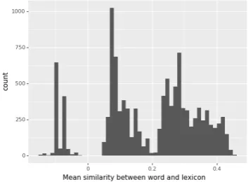
While it is not commonly the case that similarity scores follow a normal distribution, in our case, the similarity scores for words are by visual spot inspection roughly symmetric and normally dis-tributed, so we chose to characterize individual words wi by the mean and standard deviation of their similarity scores to every other word in the lexicon. Although nota prioriobvious, one possi-bility is that these metrics correlate with other lexi-cal metrics, for example, a wide standard deviation could mean that a word has a number of different ways it can be similar to other words, whereas a narrow standard deviation suggests that the word is fairly unique.
6.2 The similarity structure of the lexicon
The distributions of similarity scores show some interesting properties. Unlike the measurements of phonological neighborhood density provided in
Vaden et al.(2009), which follow a quasi-Zipfian distribution, a histogram of the mean word-lexicon similarities across the whole vocabulary shows a very different pattern. In particular, there appear to be three distinct clusters of similarity scores, as shown in Figure4.
Figure 4: Three clusters of similarity scores from Ob-served Decoder model.
Words in the first cluster, which show negative average similarity scores, were highly frequent words, typically encompassing function words (e.g. but, about, the). The second cluster ap-peared to include less high-frequency terms (e.g.
day,brain,wants). Finally, the rightmost cluster typically had higher similarity scores, represent-ing low frequency and longer words (e.g.devices,
widely,element).4 Going forward, a meta-model
4We thank our reviewers for pointing out that all of these
[image:7.595.327.504.411.541.2]will be necessary to determine what factors deter-mine a word’s mean lexicon-similarity value.
6.3 Correlation with existing phonological properties
Ideally, a new measure of phonological form should relate to measures already known to af-fect speech production. For example, a significant correlation with a particular word’s mean or stan-dard deviation similarity to all the other words in the lexicon would suggest that our measures char-acterize the lexicon in a similar way to existing measures. Similarly, because our latent represen-tations encode sequences, we expect them to cor-relate with phonotactic probability (Vitevitch and Luce, 2004). So, as a final set of analyses, we sought to test whether and to what extent the Ob-served decoder learns representations that can tell us about a word’s relationship to the rest of the lexicon.
There are two measures of interest that have re-ceived some attention in the speech production lit-erature. For the present analyses, we reference the phonological neighborhood density metrics as well as the phonotactic probability scores for words in Buckeye that are also in the Irvine Phono-tactic Online Dictionary (IPhOD; Vaden et al.,
2009). We show that our measures (both mean and standard deviation) strongly correlate with phono-tactic probability and IPhoD’s additional PND measure. This suggests that the vectors’ useful-ness extends to researchers who wish to explore the phonological similarity structure of the lexicon for psycholinguistic research.
Phonological neighborhood density. Given the importance of phonological neighborhood density (PND) in speech production (Luce and Pisoni,1998;Vitevitch and Luce, 2005;Metsala,
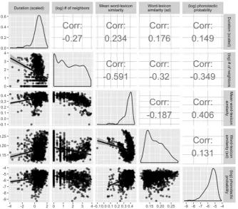
1997; Mirman, 2011), we correlated the (log) number of phonological neighbors with our latent density scores and phonetic duration. A phono-logical neighbor is a word that differs by a single sound (either an addition, a substitution, or a dele-tion;Levenshtein,1966). PND ((log) # of neigh-bors, Figure 5) has a strong negative correlation with mean word-lexicon similarity (greater mean similarity translates to fewer neighbors;ρ = -.59) while the standard deviation of word-lexicon sim-ilarity shows a non-linear relationship with neigh-borhood density.
Phonotactic probability. Phonotactic
proba-bility is a measure of the phonological typicality of a word, computed from product of uni-phone and bi-phone probabilities of that word pronunci-ation, in the same fashion that sentence probabil-ities are computed in a standard bigram language model (Vitevitch and Luce, 2004, 2005). In our final analysis, we compare the mean and standard deviation of a word’s similarity to all other word types, including alternate pronunciations of the same word, to existing measures of phonotactic probability. As with phonological neighborhood density, we see significant positive correlations be-tween our phonological similarity measures (both means and standard deviations; ρ= 0.41 andρ = 0.13, respectively) between phonotactic probabili-ties, which we visualize in Figure5.
7 Conclusion
The results presented here suggest that encoder-decoder models are a promising framework for composing segment-based representations of words. The models also characterize words’ phonological forms relative to the rest of the lex-icon. We believe that encoder-decoder models’ usefulness extends beyond that of many exist-ing approaches, as they can seamlessly gener-ate gestalt representations for out-of-vocabulary words and even nonce words. Our approach has a number of potential advantages for the cog-nitive modeling of language processing in both comprehension and production tasks, or indeed in any task that can be modeled with phonological word representations. Importantly, the encoder-decoder modeling framework is flexible, learn-ing both from observed, quasi-phonetic realiza-tions of words as well as from idealized, normative (dictionary-based) pronunciations, and allows for many variations in expressivity and computational power.
Figure 5: Correlation between a word’s phonetic duration in Buckeye, phonological neighborhood density, global word-lexicon similarity (mean and standard deviation), and phonotactic probability.
as phonological neighborhood density and phono-tactic probability. Finally, our results on the Normative-Decoder suggest that low-resource lan-guages with only a pronunciation dictionary are also a viable means of learning these represen-tations, assuming that there is a corresponding corpus of conversational data. In sum, we have demonstrated that our approach is useful for mod-eling of phonological structure.
References
Maria Antoniak and David Mimno. 2018. Evaluating the stability of embedding-based word similarities.
Transactions of the Association of Computational Linguistics, 6:107–119.
R Harald Baayen, Richard Piepenbrock, and Rijn van H. 1993. The{CELEX}lexical data base on{ CD-ROM}.Linguistic Data Consortium.
Esteban Buz and T Florian Jaeger. 2016. The (in) de-pendence of articulation and lexical planning during isolated word production. Language, Cognition and Neuroscience, 31:404–424.
W Nick Campbell. 1992. Syllable-based segmental du-ration.Talking machines: Theories, models, and de-signs, pages 211–224.
Daniel Cer, Yinfei Yang, Sheng-yi Kong, Nan Hua, Nicole Limtiaco, Rhomni St John, Noah Constant, Mario Guajardo-Cespedes, Steve Yuan, Chris Tar, et al. 2018. Universal sentence encoder. arXiv preprint arXiv:1803.11175.
Kyunghyun Cho, Bart van Merrienboer, Caglar Gul-cehre, Dzmitry Bahdanau, Fethi Bougares, Holger Schwenk, and Yoshua Bengio. 2014. Learning phrase representations using rnn encoder–decoder for statistical machine translation. Proceedings of the 2014 Conference on Empirical Methods in Nat-ural Language Processing (EMNLP), pages 1724– 1734.
Noam Chomsky. 1968. The sound pattern of English. Studies in language. Harper & Row, New York.
Yu-An Chung, Chao-Chung Wu, Chia-Hao Shen, Hung-Yi Lee, and Lin-Shan Lee. 2016. Audio word2vec: Unsupervised learning of audio segment representations using sequence-to-sequence autoen-coder. Interspeech 2016, pages 765–769.
Christopher Cieri, David Miller, and Kevin Walker. 2004. The fisher corpus: a resource for the next generations of speech-to-text. InLREC, volume 4, pages 69–71.
Alexis Conneau, Douwe Kiela, Holger Schwenk, Lo¨ıc Barrault, and Antoine Bordes. 2017. Supervised learning of universal sentence representations from natural language inference data. InProceedings of the 2017 Conference on Empirical Methods in Nat-ural Language Processing, pages 670–680.
Colin J Davis. 2010. The spatial coding model of visual word identification. Psychological Review, 117:713–758.
Gary S Dell. 1986. A spreading-activation theory of retrieval in sentence production. Psychological Re-view, 93:283–321.
Jacob Devlin, Ming-Wei Chang, Kenton Lee, and Kristina Toutanova. 2018. Bert: Pre-training of deep bidirectional transformers for language understand-ing. arXiv preprint arXiv:1810.04805.
John R Firth. 1957. A synopsis of linguistic theory, 1930-1955. Studies in linguistic analysis.
Neal P Fox, Megan Reilly, and Sheila E Blumstein. 2015. Phonological neighborhood competition af-fects spoken word production irrespective of sen-tential context. Journal of Memory and Language, 83:97–117.
Stefan Frisch. 1996. Similarity and frequency in phonology. Ph.D. thesis, Northwestern University.
Susanne Gahl, Yao Yao, and Keith Johnson. 2012. Why reduce? phonological neighborhood density and phonetic reduction in spontaneous speech. Jour-nal of Memory and Language, 66:789–806.
Stephen D Goldinger. 1998. Echoes of echoes? an episodic theory of lexical access. Psychological Re-view, 105:251–279.
Matthew Goldrick and Meredith Larson. 2008. Phono-tactic probability influences speech production.
Cognition, 107:1155–1164.
Mark Hale and Charles Reiss. 2008.The Phonological Enterprise. Studies in language. Oxford University Press, New York.
Zellig S Harris. 1954. Distributional structure. Word, 10:146–162.
Sepp Hochreiter and J¨urgen Schmidhuber. 1997. Long short-term memory. Neural computation, 9(8):1735–1780.
George Houghton and Tom Hartley. 1996. Parallel models of serial behaviour: Lashley revisited. Psy-che: An Interdisciplinary Journal of Research on Consciousness.
Keith Johnson. 2004. Massive reduction in conver-sational american english. In Spontaneous speech: Data and analysis. Proceedings of the 1st session of the 10th international symposium, pages 29–54. Citeseer.
Armand Joulin, Edouard Grave, Piotr Bojanowski, and Tomas Mikolov. 2017. Bag of tricks for efficient text classification. InProceedings of the 15th Con-ference of the European Chapter of the Association for Computational Linguistics: Volume 2, Short Pa-pers, volume 2, pages 427–431.
Diederik P. Kingma and Jimmy Ba. 2015. Adam: A method for stochastic optimization. In Proceed-ings of the 3rd International Conference on Learn-ing Representations (ICLR).
Thomas K Landauer and Susan T Dumais. 1997. A so-lution to plato’s problem: The latent semantic anal-ysis theory of acquisition, induction, and representa-tion of knowledge. Psychological Review, 104:211– 240.
Jey Han Lau and Timothy Baldwin. 2016. An empiri-cal evaluation of doc2vec with practiempiri-cal insights into document embedding generation. In Proceedings of the 1st Workshop on Representation Learning for NLP, pages 78–86.
Quoc Le and Tomas Mikolov. 2014. Distributed repre-sentations of sentences and documents. In Interna-tional conference on machine learning, pages 1188– 1196.
Willem JM Levelt, Ardi Roelofs, and Antje S Meyer. 1999. A theory of lexical access in speech produc-tion. Behavioral and Brain Sciences, 22:1–38.
Vladimir I Levenshtein. 1966. Binary codes capable of correcting deletions, insertions, and reversals. In
Soviet Physics Doklady, volume 10, pages 707–710.
Paul A Luce and David B Pisoni. 1998. Recognizing spoken words: The neighborhood activation model.
Ear and Hearing, 19:1–36.
Laurens van der Maaten and Geoffrey Hinton. 2008. Visualizing data using t-sne. Journal of Machine Learning Research, 9:2579–2605.
Viorica Marian, James Bartolotti, Sarah Chabal, and Anthony Shook. 2012. Clearpond: Cross-linguistic easy-access resource for phonological and orthographic neighborhood densities. PloS one, 7(8):e43230.
William Marslen-Wilson and Paul Warren. 1994. Lev-els of perceptual representation and process in lexi-cal access: words, phonemes, and features. Psycho-logical review, 101(4):653.
Jamie L Metsala. 1997. An examination of word fre-quency and neighborhood density in the develop-ment of spoken-word recognition. Memory & Cog-nition, 25(1):47–56.
Daniel Mirman. 2011. Effects of near and distant se-mantic neighbors on word production. Cognitive, Affective, & Behavioral Neuroscience, 11(1):32–43.
Graham Neubig, Chris Dyer, Yoav Goldberg, Austin Matthews, Waleed Ammar, Antonios Anastasopou-los, Miguel Ballesteros, David Chiang, Daniel Clothiaux, Trevor Cohn, Kevin Duh, Manaal Faruqui, Cynthia Gan, Dan Garrette, Yangfeng Ji, Lingpeng Kong, Adhiguna Kuncoro, Gaurav Ku-mar, Chaitanya Malaviya, Paul Michel, Yusuke Oda, Matthew Richardson, Naomi Saphra, Swabha Swayamdipta, and Pengcheng Yin. 2017. Dynet: The dynamic neural network toolkit. arXiv preprint arXiv:1701.03980.
John J Ohala. 1990a. The phonetics and phonology of aspects of assimilation. Papers in Laboratory Phonology, 1:258–275.
John J Ohala. 1990b. There is no interface between phonology and phonetics: a personal view. Journal of Phonetics, 18:153–171.
F. Pedregosa, G. Varoquaux, A. Gramfort, V. Michel, B. Thirion, O. Grisel, M. Blondel, P. Pretten-hofer, R. Weiss, V. Dubourg, J. Vanderplas, A. Pas-sos, D. Cournapeau, M. Brucher, M. Perrot, and E. Duchesnay. 2011. Scikit-learn: Machine learning in Python. Journal of Machine Learning Research, 12:2825–2830.
Janet Breckenridge Pierrehumbert. 1980. The phonol-ogy and phonetics of English intonation. Ph.D. the-sis, Massachusetts Institute of Technology.
Mark A Pitt, Keith Johnson, Elizabeth Hume, Scott Kiesling, and William Raymond. 2005. The buck-eye corpus of conversational speech: labeling con-ventions and a test of transcriber reliability. Speech Communication, 45:89–95.
Uriel Cohen Priva. 2015. Informativity affects con-sonant duration and deletion rates. Laboratory Phonology, 6(2):243–278.
Radim ˇReh˚uˇrek and Petr Sojka. 2010. Software Frame-work for Topic Modelling with Large Corpora. In
Proceedings of the LREC 2010 Workshop on New Challenges for NLP Frameworks, pages 45–50, Val-letta, Malta. ELRA. http://is.muni.cz/
publication/884893/en.
M. Schuster and K.K. Paliwal. 1997. There is no in-terface between phonology and phonetics: a per-sonal view. IEEE Transactions on Signal Process-ing, 45:2673–2681.
Mark S Seidenberg and James L McClelland. 1989. A distributed, developmental model of word recogni-tion and naming. Psychological Review, 96:523– 568.
Christine A Sevald and Gary S Dell. 1994. The sequen-tial cuing effect in speech production. Cognition, 53:91–127.
Scott Seyfarth. 2014. Word informativity influ-ences acoustic duration: Effects of contextual pre-dictability on lexical representation. Cognition, 133(1):140–155.
Daragh E Sibley, Christopher T Kello, David C Plaut, and Jeffrey L Elman. 2008. Large-scale modeling of wordform learning and representation. Cognitive Science, 32(4):741–754.
Kenneth N Stevens and Sheila E Blumstein. 1981. The search for invariant acoustic correlates of phonetic features. Perspectives on the study of speech, pages 1–38.
Lidia Su´arez, Seok Hui Tan, Melvin J Yap, and Win-ston D Goh. 2011. Observing neighborhood effects without neighbors. Psychonomic Bulletin & Review, 18(3):605–611.
Ilya Sutskever, Oriol Vinyals, and Quoc V Le. 2014. Sequence to sequence learning with neural net-works. InAdvances in Neural Information Process-ing Systems, pages 3104–3112.
Harry Tily and Victor Kuperman. 2012. Rational phonological lengthening in spoken dutch. The Journal of the Acoustical Society of America, 132(6):3935–3940.
Rory Turnbull, Scott Seyfarth, Elizabeth Hume, and T Florian Jaeger. 2018. Nasal place assimilation trades off inferrability of both target and trigger words. Laboratory Phonology: Journal of the As-sociation for Laboratory Phonology, 9(1).
Kenneth I Vaden, HR Halpin, and Gregory S Hickok. 2009. Irvine phonotactic online dictio-nary, version 2.0. [data file]. Available from http://www.iphod.com.
Michael S Vitevitch and Paul A Luce. 2004. A web-based interface to calculate phonotactic probabil-ity for words and nonwords in english. Behav-ior Research Methods, Instruments, & Computers, 36:481–487.
Michael S Vitevitch and Paul A Luce. 2005. In-creases in phonotactic probability facilitate spoken nonword repetition. Journal of Memory and Lan-guage, 52:193–204.
Sida Wang and Christopher D. Manning. 2012. Base-lines and bigrams: simple, good sentiment and topic classification. Proceedings of the 50th Annual Meet-ing of the Association for Computational LMeet-inguis- Linguis-tics: Short Papers, 2:90–94.