Analytical Solutions of the 1D Dirac Equation Using the Tridiagonal Representation Approach

(1)

http://www.scirp.org/journal/jamp ISSN Online: 2327-4379 ISSN Print: 2327-4352

DOI: 10.4236/jamp.2017.510172 Oct. 31, 2017 2072 Journal of Applied Mathematics and Physics

Analytical Solutions of the 1D Dirac

Equation Using the Tridiagonal

Representation Approach

Ibsal A. Assi

1*

, Hocine Bahlouli

2,3

1_{Department of Physics and Physical Oceanography, Memorial University of Newfoundland, St. John’s A1B3X7, NL, Canada} 2_{Physics Department, King Fahd University of Petroleum & Minerals, Dhahran, KSA}

3_{Saudi Center for Theoretical Physics, Jeddah, KSA}

Abstract

This paper aims at extending our previous work on the solution of the one-dimensional Dirac equation using the Tridiagonal Representation Ap-proach (TRA). In the apAp-proach, we expand the spinor wavefunction in terms of suitable square integrable basis functions that support a tridiagonal matrix representation of the wave operator. This will transform the problem from solving a system of coupled first order differential equations to solving an al-gebraic three-term recursion relation for the expansion coefficients of the wa-vefunction. In some cases, solutions to this recursion relation can be related to well-known classes of orthogonal polynomials whereas in other situations so-lutions represent new class of polynomials. In this work, we will discuss vari-ous solvable potentials that obey the tridiagonal representation requirement with special emphasis on simple cases with spin-symmetric and pseudos-pin-symmetric potential couplings. We conclude by mentioning some poten-tial applications in graphene.

Keywords

Dirac Equation, Tridiagonal Representation, Three-Term Recursion Relation, Orthogonal Polynomials, Energy Spectrum, Isospectral Potentials,

Spin-Symmetric Coupling, Pseudo-Spin-Symmetric Coupling, Graphene

1. Introduction

The basic equation of relativistic quantum mechanics was formulated by Paul Dirac in 1928 in a way consistent with special relativity [1]. This equation de-scribes the behavior of weakly coupled electrons at high speeds or strongly

How to cite this paper: Assi, I.A. and Bahlouli, H. (2017) Analytical Solutions of the 1D Dirac Equation Using the Tridia-gonal Representation Approach. Journal of Applied Mathematics and Physics, 5, 2072-2092.

https://doi.org/10.4236/jamp.2017.510172 Received: October 3, 2017

Accepted: October 28, 2017 Published: October 31, 2017 Copyright © 2017 by authors and Scientific Research Publishing Inc. This work is licensed under the Creative Commons Attribution International License (CC BY 4.0).

(2)

DOI: 10.4236/jamp.2017.510172 2073 Journal of Applied Mathematics and Physics

coupled electrons such as in the case of core electron states in heavy atoms. Among the benefits of this relativistic formulation, it is the natural emergence of the electron spin and the prediction of the existence of an antiparticle partner to the electron, the positron, which was discovered experimentally few years later. The physics and mathematics of the Dirac equation is very rich, illuminating and providing a theoretical framework for different physical phenomena that are not present in the nonrelativistic regime such as the Klein paradox [2]. In addition, Dirac equation emerges in the study of the transport properties in graphene, which makes it important for future applications. Graphene is the first truly two dimensional system whose carriers exhibit a relativistic-like behavior. Electrons in graphene are described by a massless two dimensional relativistic Dirac equa-tion that gives rise to a gapless energy dispersion near the K and K’ points of the first Brillouin zone. So in this context, graphene represents a test bed for many relativistic phenomena such as Klein tunneling that could be observed with car-rier having speeds one thousand time smaller than the speed of light [3] [4] [5].

Exact solutions of the Dirac equation with a given potential configuration are limited and not trivial [6] [7] [8] [9] [10] compared to the nonrelativistic Schrödinger equation. In fact, the Dirac Hamiltonian being a matrix in the spi-nor space allows for more structure in the potential interaction. The terminology given to relativistic problems such as the “Dirac-Coulomb”, “Dirac-Oscillator”, “Dirac-Morse”, ∙∙∙ etc. refers to the Dirac equation that reduces to an effective Schrödinger-like equation with the named potential for the large spinor compo-nent. Different approaches were developed to generate exact solutions to the Di-rac equation such as supersymmetric quantum mechanics [11], Darboux trans-formation [12] and factorization method [13] to mention only few.

This paper is an expanded version of our letters [14] with further develop-ments and applications in which we use the J-matrix inspired Tridiagonal Re-presentation Approach (TRA). The basic idea of the approach is to write the spinor wavefunction as a bounded infinite series with respect to a suitably cho-sen square integrable basis function as

( )

m

( ) ( )

m m

x f x

ε

ψ

=

∑

ε φ

where

{

fm

( )

ε

}

_m₀

∞

= is a set of expansion coefficients that are functions of the

energy and potential parameters and

{

m

( )

}

₀ m x

φ

∞

= is a complete set of spinor

basis functions that carry only kinematic information. Using this form of the spinor wavefunction in the stationary wave equation,

(

H−

ε ψ

)

=J

ψ

=0,

where H is the Dirac Hamiltonian and requiring that the matrix representation of the wave operator, Jn m, =

φ

n

(

H−

ε φ

)

m , be tridiagonal and symmetric so

that the action of the wave operator on the elements of the basis is allowed to take the general form

(

H−E

)

φ

n ∼

φ

n +

φ

n−1 +

φ

n+1 . This requirement

transforms the wave equation to the following three-term recursion relation for

( )

{

fm

ε

}

m 0

∞

= [15]:

( )

, , 1 1 , 1 1 0

n n n n n n n n n

(3)

Thus, the problem now reduces to solving this three-term recursion relation which is equivalent to solving the original wave equation. Of course, this equa-tion can be solved in different ways in mathematics [16] [17]. Sometimes solu-tions of Equation (1.1) can be written in a closed form by direct comparison to well-known orthogonal polynomials. However, in other cases this recursion re-lation does not correspond to any of the known orthogonal polynomials giving rise to new class of orthogonal polynomials. The challenge will then be to write these solutions in a closed form and find the properties of the associated ortho-gonal polynomials such as the weight function, generating function, spectrum formula, asymptotics, zeroes, etc.

In the following section, we introduce the general formulation of the problem and show how to calculate the matrix elements of the Dirac wave operator in a general basis. Then we consider two important choices of bases depending on the configuration space of the problem. One is written in terms of the Jacobi po-lynomials and the other is written in terms of Laguerre popo-lynomials. In the third section, we present various examples of exactly solvable potentials with special focus on possible applications. We give our conclusions and discuss future work in the last section.

2. Theoretical Modeling

The most general form of 1D time-independent Dirac equation in the presence of scalar potential S x

( )

, two-component (time, space) vector potential

( )

x =

(

V x U x

( ) ( )

,

)

A and pseudo-scalar potential W x

( )

can be written in the

following form (in the relativistic units = =c 1):

( )

d d d

d

m S x V x W x iU x

x x

x

x x

W x iU x m S x V x

x

ψ ψ

ε

ψ ψ

+ +

− −

 ₊ ₊ ₊ ₋ 

 _ _ _ _

 _ _= _ _

 ₊ ₊ _{− −} ₊ _ _ _ _

 

 

−

(2.1)

where

ε

is the energy and Ψ

( )

x =

(

ψ

+

( )

x ,

ψ

−

( )

x

)

t is the two-component

spinor wavefunction. The space component of the vector potential can be gauged away to simplify the problem using a unitary transformation

( )

e

i x

x

ψ

±

→

− Λ

ψ

±

provided that the phase function Λ₍_x_{) obey the}

rela-tionship dΛ dx U x=

( )

, hence from now on we set U(x) = 0 in our equations.

Our strategy then is to write the spinor components as an expansion over a complete basis set

( )

n

( ) ( )

n n

x f x

ψ

± ₌

∑

ε φ

±

where

{

φ

n

( )

x

}

_n₀

∞ ±

= is now a two-component spinor basis. The matrix elements,

, n m

J associated with (2.1) is written below:

(

)

,

d d

n m n m n m n m

n m n m

J H Q Q

W W

x x

φ ε φ φ φ φ φ

φ φ φ φ

+ + − −

+ −

+ − − +

= − = +

   

+ _− + _ + _ + _

   

(4)

where Q_±=V x

( ) ( )

±S x ± −m

ε

and

φ

n

( )

x

(

φ

n

( ) ( )

x ,

φ

n x

)

t

+ −

= is the spinor

wavefunction.

In the presence of symmetry, we get more solutions to Equation (2.1). These symmetries include the spin-symmetric coupling in which V x

( )

=S x

( )

, the

pseudospin symmetric coupling which requires V x

( )

= −S x

( )

, and the

pres-ence of the scalar potential alone, i.e. V x

( )

=W x

( )

=0. We have discussed all

the possible symmetries in Section 3. In these symmetries, the problem reduces to solving an effective 1D Schrödinger-like equation which has been treated us-ing the TRA in the past [18] [19] [20] [21], and very recently in [22]. In what follows, we will discuss the situation in which there is no relationship between the potentials in Equation (2.1).

We start here by relating the spinor components using Equation (2.1), in ab-sence of U(x), as follows:

( )

1 d

( )

d

x W x

m S V x

ψ ψ

ε

− ₌  ₊  +

 

+ + −   (2.3)

We refer sometimes to

ψ

+

( )

x as the “larger” component due to the

domi-nator in (2.3). The general case we refer to holds when we have V(x) alone or

V(x) and S(x) together with or without W(x) with no symmetry between V(x) and S(x). To simplify the problem, we relate the corresponding basis functions through the kinetic balance relation[23]:

( )

d

( )

d

n x W n x

m x

η

φ φ

ε

− ₌  ₊  +

 

+   (2.4)

where η is just a real dimensionless constant and

ε

≠ −m which means that

this solution will cover only the positive energy space. Using Equation (2.4) in (2.2) with the coordinate transformation x→y x

( )

, we can write the matrix

elements of the wave operator, J, as follows:

(

)

2 2

, 2 2

2

d d

n m n m

n m

y

J y

m y y y

m

Q W W

m

η _φ _φ

ε

η _φ ε _φ

ε η

+ +

+

 ′′ 

′

= − _ + _

′

+ _ _

 + _′ 

+ _ + − _

+ _ _

(2.5)

where the prime over the variable stands for the derivative with respect to x, i.e. d

d

W W

x

′ = _{The coordinate transformation is made such that we make the do-}

main of the Hamiltonian compatible with the domain of the basis functions, see

Table 1. The next step is to use basis functions that make (2.5) tridiagonal and symmetric. We usually use two important bases which are mentioned below:

1) Laguerre Basis:

( )

e y

( )

n y A yn Ln y

α β ν

φ

+ ₌ − _(2.6)

where Ln

( )

y

ν _{is the generalized Laguerre polynomial of order}

n in y,

(

)

(

)

1 1

n

n A

n

ν

Γ + =

Γ + + is just a normalization constant, and

{

α β ν

, ,

}

are real

(5)

[image:5.595.214.536.500.626.2]

DOI: 10.4236/jamp.2017.510172 2076 Journal of Applied Mathematics and Physics Table 1. Few interesting coordinate transformations that are very useful in our approach which will be used to obtain different class of solvable potentials.

Transformation equation Domain mapping: x→y Basis

y=λx

[ [ ] [

0,∞ → 0,∞

Laguerre

( )2

y= λx ℜ →

] [

0,∞

e x

y=µ −λ ℜ →

] [

0,∞

( )

tanh

y= λx ℜ → −

[ ]

1,1

Jacobi

1 2e x

y= − −λ

[ [ [ ]

0,∞ → −1,1

( )

cos

y= λx

[

0,π 2

] [ ]

→ −1,1

( )2

2 1

y= x L −

[ ] [ ]

0,L → −1,1

( )

2

2 tanh 1

y= λx −

[ [ [ ]

0,∞ → −1,1

2) Jacobi Basis:

( )

(

) (

)

( ,)

( )

1 1

n y An y y Pn y

α β µ ν

φ+ ₌ ₋ ₊ _(2.7)

where

(

1

) (

(

) (

)

2 1 1 1

1 1

2

n

n n n

A

n n

µ ν

ν

µ

+ +

+ + + Γ + Γ + + + =

Γ + + Γ + + is just a normalization

constant, y∈ −

[ ]

1,1 and P_n(µ ν, )

( )

y is Jacobi polynomial of order n. The

para-meters

{

α β µ ν

, , ,

}

, with

µ ν > −

,

1

, are real numbers.

An interesting task for the motivated reader is to use these bases to verify that Equation (2.3) leads to Equation (2.4), i.e. the tridiagonal representation of Jn m,

cannot be made unless we use the kinetic balance relation. In this section, we do the calculations in Laguerre basis, while the calculations in Jacobi basis can be found in Appendix B. This gives the following form of the matrix elements:

(

)

( )

2 2

, 2

2

d d

e 1

d d

e y

n m

n m n m

y

n m

n n

A A

J L y y y L

m y y

A A y

L y G y L

m y

ν ν ν

η κ _ν

ε

η κ

ε

−

 

= − _ + + − _

+ _ _

−

′ +

(2.8)

where,

( )

(

)

(

)

(

)

2 2

1

2

m a

y

G y W W Q

y y

a b b y

ε α α

η

αβ β α β β

+

+ + −

 

′

= _ − + _−

′  

+ + − − −

(2.9)

Using the properties of

L

n

ν_{(A1), (A3), and (A4), we impose the following}

constraints:

1) We use the coordinate transformation that satisfies y′ =

κ

ya bye , for reals

{

a b, ,

κ

}

. This form is compatible with the Laguerre weight function in (2.6) and eases the measure transformation.

(6)

ensure the tridiagonal representation of the first matrix element in (2.8). 3) G y

( )

=

ρ

y+

σ

, for reals ρ and

σ

, to ensure the tridiagonal

represen-tation of the last matrix element in (2.8).

Thus, the tridiagonal form of Jn m, becomes:

(

)

{

(

)

(

)

}

2

, ,

, 1 , 1

2 1

( 1) 1

n m n m

J n n

m

n n n n

ηκ _ν _{ρ σ} _δ

ε

ρ ν δ ₊ ν δ ₋

= _ + + + + _

+

 

− _ + + + + + _

(2.10)

The potentials that allow (2.10) to hold must be chosen such that:

(

)

(

)

(

)

2 2

1

2

m a

y

y W W Q

y y

a b b y

ε α α

ρ σ

η

αβ β α β β

+

+ + −

 

′

+ = _ − + _−

′  

+ + − − −

(2.11)

We will discuss all the possible symmetries in Section 3.

3. Results and Discussions

This section is divided into three parts organized as follows. In Section 3.1, we expose different results related to graphene. In Sections 3.2, we discuss the set of possible solvable potentials in presence of spin symmetries. Then we move to Section 3.3 to expose some results on the general case.

3.1. Scalar Potential

In this situation we consider W x

( )

=V x

( )

=0. Applying the unitary

transfor-mation _eiπ4σy, where y

σ _{is the 2 × 2 Pauli matrix} 0

0

i i

−

 

 

 , on Dirac

Hamil-tonian in Equation (2.1), this gives the following form of the wave equation:

( )

d 0

d d

0 d

m S

x x

x

x x

m S

x

χ χ

ε

χ χ

+ +

− −

 _{+ +} 

 _ _ _ _

 _ _= _ _

₋ _{+ +} _ _ _ _

 

 

(3.1.1)

where χ =_eiπ4σy ψ . The reason behind this transformation is that Equation

(3.1.1) is equivalent to Dirac-Weyl equation for an electron in graphene moving under the influence of an external magnetic field acting perpendicular to the plane of the graphene sheet. To see the correspondence, we write down the Di-rac-Weyl equation which reads [24] [25]1_:

( )

,

( )

,

F

e

v x y E x y

c

 

⋅_ + _ Ψ = Ψ

p A

σ _(3.1.2)

where vF is the Fermi speed,

(

)

T ,

x y

σ σ

=

σ

is the vector Pauli matrices,

,

i

x y

 ∂ ∂ 

= − _{∂ ∂} 

 

p  is the 2D momentum operator, e is the electron’s charge, c is

(7)

the speed of light, A is the two-vector potential, and E is the energy

eigen-value. Now, choosing the z-axis normal to the graphene sheet, then the magnetic field could be generated from the two-vector potential in the Landau gauge

( )

(

0,A_y x , 0

)

=

A as

( )

(

0, , 0 ,

)

(

0, 0, ( ) ,

) ( )

d

y y

A

A x B x B x

x

= = =

A B (3.1.3)

This gauge suggests that the spinor is separable as _Ψ

( )

_{x y}, ₌eiky ψ

( )

_x

(translational symmetry). This will reduce Equation (3.1.2) to Equation (3.1.1) with the following maps:

m→k, y

e

S A

c →

 , ε =E vF , and

χ

→

ψ

If we define F x

( )

= +m S x

( )

, we can now relate the spinor wavefunction

components in Equation (3.1.1) as follows:

( )

1 d

( )

d

x F x x

x

χ χ

ε

± ₌ _± ₊ 

 

 

 _(3.1.4)

The constraint in Equation (3.1.4) allows us to break Dirac equation into two effective Schrödinger equations for each spinor component which we write down in compact form as follows:

2

2 d

2 2 0

dx U E χ

±

 

− + =

 

   (3.1.5)

where

2 2

F F

U= ± ′, and

2 2

E=

ε

, with d

d

F F

x

′ = _{. Consequently, we just need}

to solve the effective Schrödinger Equation (3.1.5) for any component and find the other spinor component using the relation in (3.1.4). However, we need to stress that each solution of (3.1.5) will cover part of the energy space comple-mentary to the other one. Luckily, Schrödinger equation has been treated in the past, using the TRA, by different authors including Alhaidari and Bahlouli [15] [18] [19] [20] [21]. We have tabulated few of the solvable potentials of Equation (3.1.5), which were treated by the TRA, in Table 2. We should point out that the situation with S= =V 0 is mathematically similar to the previous case which

results, again, in having two Schrödinger equations for each spinor component as in Equation (3.1.5) with _U=

(

_W2±_W′

)

₂ and _E=

(

ε2−_m2

)

₂. Next,

we-will discuss different situations that we-will be useful for graphene system.

As a first example, we consider the following hyperbolic magnetic field bar-rier:

( )

0

( )

2 cosh

B B x

x α

= _(3.1.6)

where B0 and

α

are constants. This case corresponds to m=k and

( )

0tanh

S=S

α

x , with S₀=eB₀ αc. Comparison to Schrödinger equation,

(8)

[image:8.595.62.539.88.459.2]

DOI: 10.4236/jamp.2017.510172 2079 Journal of Applied Mathematics and Physics Table 2. Some of the solvable potentials for Schrödinger equation which were obtained in the past using the TRA [14] [23] [28].

( )

V x Domain _(x) En ( , n) m m( ) ( )n m

x E f E x

ψ =

∑

φ _Constraints

( )

2

1 2

B l l A

x x

+ +

+

[ [

0,∞

2

1

2 2 1

A

n ν

 

−  ₊ ₊ 

 

( )

1 2 2

ex n x A xn L xn

ν ν

φ ₌ + −

(

)

2

1 2 l 1 2 2B

ν = − + + +

1

ν> −

( )

4 2 2 1 2 1 2

B l l x

x

λ + + +

]

−∞ ∞,

[

2

(

)

2n 2

λ + +ν _{( )} 3 _{( )}

2 2 4_ex n x A xn L xn

ν ν

φ + ₋

=

(

)

2

1 2 l 1 2 2B

ν = − + + +

1

ν > −

( ) 2 2 2 e e 2 2 x x V x

A λ λ

λ  −  µ − 

= _ + _{ } _  

]

−∞ ∞,

[

2 2 1 2 2 A n λ µ   −  + +   

( )

(

)

1 1

2 e 2 2

e e x e

A A

n x n

x

n x An Ln

λ

µ µ µ λ

ψ − + + ₋ − + + µ ₋

= µ λ >, 0

(

)

2

e 1

ex 1 x

C A

λ

λ ₋ + −

[ [

0,∞

( ) 2 2 2 2 1 1 8 2 2 n A C E n n λ λ ν ν    + −  = −  + + ₊   +      ( ) ( )( ) ₍ ₎( ) ( )_{( )}

1 2 1 2

,

1 1

n n

n

x A y y

P y

ν µ

µ ν

ψ + +

= − + ×

(

)

2 2 1 8

C=λ ν −

, 1

µ ν> −

1 2e x

y= − −λ

( ) ( )

( )

2

tanh

cosh

V x C x

A x λ λ = +

]

−∞ ∞,

[

2 2 2 2 2 2

n n n

C

E λ ϑ ϑ

λ −

 _ _ 

= −  +_ _ 

 

 

( ) ( ) (2 ) 2 ( , )_{( )}

1 n 1 n n n

n x An y y Pn y

ν µ µ ν

ψ = − +

( )

tanh

y= λx , λ >0

( ) (2 )2

2 2

C= λµ − λν

1 2

n n D

ϑ =_ + − λ_

 

( ) (2 )2

2 2

n

E = − λµ − λν

(

)

0cos

V k xλ

[ ]

0,L See [28] ( ) (1 2, 1 2) ( )

cos

n x Pn k x

ψ _∝ ± ± _ λ _

  π

L

λ=

0,1, 2, 3,

k= 

( )

0

(

( )

0

)

2 2

( )

0 0 2 1 2 tanh 2 cosh S S

U x k S kS x

x

α

 −  = _ + + + _    

 _(3.1.7)

This potential is called the hyperbolic Rosen-Morse potential which was treated using the TRA in [15]. Using the energy spectrum of this potential (See

Table 2), we write the energy spectrum of an electron in graphene in this hyperbolic barrier as follows:

2

2 2

2 2 2 2 2 2 0

0 2

1 1

2 2

n F

kS

v k S n n

ε

α

γ

α

− _ _ _ _ _ _  = + − _ + − _ +_ _ _ + − _           

 (3.1.8)

where 2 0

(

0

)

2

1 4

S S α

γ

α −

= + _and

(

)

2 0 0

4

S S −

α

> −

α

. This result agrees with the

result obtained in [3]. The upper component of the spinor wavefunction is now written as [15]:

( )

(

( )

)

2

(

( )

)

2 ( , )

(

( )

)

, 1 tanh n 1 tanh n n n tanh eiky

n x y An x x Pn x

ν µ µ ν

χ

+ ₌ ₊

α

₋

α

_(3.1.9)

where

(

0

)

1 2

n n kS

µ

ϑ

α

= − − _,

ν

_n 1 2

(

ϑ

_n kS₀

)

α

= − − _, _{2 2}2

2 n n F v ε ϑ =

 , and

(

) (

)

(

) (

)

1

2 1 1 1

1 1

2

n

n n n

A

n n

µ ν

α

µ ν

ν

µ

+ +

+ + + Γ + Γ + + + =

(9)

con-DOI: 10.4236/jamp.2017.510172 2080 Journal of Applied Mathematics and Physics

stant. The lower spinor component can be easily calculated using Equation (3.1.4).

Another interesting example we mention here is the case when the magnetic barrier takes the following exponentially decaying form:

0e

x

B=B −α (3.1.10)

where B0 and

α

are constants with α >0. This case corresponds to a scalar

potential of the form 0e

x

S=S −α , where S₀= −eB c₀ α. Now, using Equation

(3.1.5), we find that the Schrödinger potential reads:

( )

2 2 2

(

)

0 0

1

2 e 2 e

x x

S S k

U x = _k + − α+ −α −α_ (3.1.11)

This is simply the 1D Morse oscillator potential, up to a constant, which was treated using the TRA for Schrödinger equation by Alhaidari in [15]. Using the results in [15], we write the energy eigenvalues for Dirac-Weyl equation as fol-lows:

2

2 2 2 2 2 1

2

n vF k n

γ

ε α

µ

 

= − _ + + _

 

 (3.1.12)

where 0

(

)

2 2

S k

γ

= −

α

_and

µ

= 2S0

α

. The upper component of the

spi-nor wavefunction reads:

( )

(

e

)

2

(

)

, e e e

x

x _x

n n n

iky

x y A L

α

αν µ _ν _α

χ

+ ₌ − + −

µ

− _(3.1.13)

where ν 2γ 2n 1

µ

= + + _{. Our results in this example agree with previous findings}

[3].

One last example we mention in this section is what we call the Hulthén bar-rier in which the magnetic field takes the following form:

( )

(

0

)

2

e

e 1

x

x B B x

α

=

− (3.1.14)

where B0 and α >0 are constants. Following the same procedure, this will be

the situation when the scalar potential is

( )

0 e x 1

S

S x = _α

− . The associated

super-symmetric potential (Schrödinger potential) now reads:

( )

(

)

(

0 0

)

2 0

(

)

2

2 1 e 1

1 e

2 _x x

S S S k

U x _α k

α

α α

− −

+ +

 

 

=

 

 − + − + 

 _(3.1.15)

The potential in (3.1.15) is the generalized Hulthén potential which was treated in the TRA in [15]. Based on the results obtained in [15], we write the energy eigenvalue of Dirac-Weyl equation for this situation as follows:

(

)

2

2 2

2 2 2 2 1 2

1

4 2

2

n vF k n

n

γ ω α

α ν

ε _ν

 

 + − 

= − _ + + _

+

 + 

 

(10)

where

(

0

)

2 2

0 1

2 2 4

S S α α ν

ω= = _ − 

 −  ,

(

)

0 2 2

S k

α

γ

= − _{, and}ν > −1. Now, we

write down the spinor component as follows:

( )

2

(

)

( )1 2

( )

( 1 2) ( _, )

(

)

2

, 2 1 e e e 1 2e

n

n _n

x x iky x

n x y An Pn

ν µ _ν _µ

µ ν

α α α

χ+ ₌ + + ₋ − + − + ₋ − _(3.1.17)

where µ > −n 1 and satisfies

(

)

2

2 2

2

1 1 1

1

2 4 2

2

n _n

n

γ ω α

µ ν ν    −  + +  _{ =} ₊ ₊     ₊   _ ₊ _   . We

leave it to the interested reader to calculate the lower component using Equation (3.1.4). Up to our knowledge, this situation was not treated in the past. Note that for very large values of x the barrier will behave similarly to the previously men-tioned case. It is obvious that all of the previous systems have finitely many bound states as shown in the spectrum formulas.

We have also solved other interesting situations in which the magnetic field is constant, singular 2

1

x , and few other cases are summarized in Table 3.

3.2. Spin-Symmetry and Pseudo-Spin Symmetry

Defining Σ = +V S and ∆ = −V S, we refer to the spin-symmetric coupling

the situation where we have ∆ =0, and the pseudo spin symmetric coupling for

Table 3. List of magnetic field configurations in graphene with the energy eigenvalue and the supersymmetric potential (Schrödinger potentials) of each case [14].

( )

B x U x( ) 2

n ε

0

B

(

)

2

1

2 x k 2

γ

γ + +

0

eB c

γ= 

( )

2 2

2 2 1

F

v _ γ+ ω n+ _

 

2 2

m

γ = ω

0 2 B x

(

)

2 2 1 2 2 k k x x

γ γ− γ

+ +

0

eB c γ= − 

2 2 2 2

1 2 1 F v k n γ ν  _ _ −   ₊ ₊       

(

)

2 1 1

ν= γ− > −

( ) _{( )}0

2 cos B B x x λ =

( )

(

)

( )

2 2

0 0 2

0

0tan sec

2 2

S S

k S

kS λx +λ λx

− ₊ ₊

where S0=eB c0 λ

2 2 2 2 2 2

0 2 2 2 0 2 1 2 1 2 F

v k S n D

kS n D λ λ λ λ λ −  _ _ − + + −  _ _       − _ _ _ + − _   

where 2

(

)

2

0 0 4

D =S S +λ λ+ and

(

)

2

0 0 4

S S +λ > −λ

( ) _{( )}0

2 sinh B B x x λ = ( ) ( ) ( ) 2 2 0 0 0

0coth 2

2 2 sinh

S S k S kS x x λ λ λ − − ₋ ₊

where S0= −eB c0 λ

2 2 2 2 2 2

0 2 2 2 0 2 1 2 1 2 F

v k S n D

kS n D λ λ λ λ λ −  _ _ − − + −  _ _       − _ _ _ + − _   

where 2

(

)

2

0 0 4

D =S S −λ λ+ and

(

)

2

0 0 4

[image:10.595.208.542.73.207.2]

(11)

which Σ =0.2 These cases are very useful in nuclear physics [26] [27] [28]. For

the case when ∆ =0, we use Equation (2.1) to write an equation for the upper

spinor component which reads:

2

2 1 d

2 dx Uss ψ Eψ

+ +

 

− + =

 

  (3.2.1)

where

(

)

2 2

ss

W W

U = − ′+

ε

+m V ,

2 2

2

m

E=

ε

− , and d

d

W W

x

′ = _{. Thus, we need}

to solve Schrödinger Equation (3.2.1) for

ψ

+ _{and then use (2.1) to compute}

ψ

−_{. As discussed in previous section, we will rely on the obtained solutions of}

Schrödinger equation using the TRA, where we tabulated few of these solvable potentials in Table 2, to obtain solvable potentials in these cases. Similarly, one can follow the same procedure for Σ =0 , which results in an effective

Schrödinger equation for the spinor lower component which is shown below:

2

2 1 d

2 dx Ups ψ Eψ

− −

 

− + =

 

  (3.2.2)

where 2

(

)

2Ups=W +W′+2

ε

−m V , and

2 2

2E=ε −m . In what follows, we

ex-pose different examples in which (3.2.1) and (3.2.2) are exactly solvable in the TRA in the presence of the potentials Uss and Ups, respectively.

The first example of solvable potentials we would like to mention here is the case when

( )

2

0

V x = −S x =V x with W x

( )

=0. The effective Schrödinger

equation in this case reads:

(

)

2

2 0 2

1 d

2 dx ε m V x ψ Eψ

− −

 

− + − =

 

  (3.2.3)

where 2 2

2E=ε −m . This is equivalent to Schrödinger equation for the

Har-monic oscillator with “frequency”

ω

=

2

(

ε

−

m V

)

0 . The basis components are

written in Laguerre basis as

( )

1 2 2 22

( )

2 2

e

x

n

x

A

n

x

L

n

x

ν λ ν

φ

−

=

λ

+ −

λ

, which was treated in the TRA, see [15], with ν = ±1 2. Using the energy spectrum for the

Harmonic oscillator obtained in the TRA, we write the bound states spectrum formula for this potential configuration in Dirac equation as follows:

(

) (

)

2 2

0

2 2

2

1

n

m

n

m V

n

ε

−

=

ε

−

+ +

ν

(3.2.4) where ε >m V, 0>0, and n=0,1, 2,. It is well known that Laguerre and

Her-mite polynomials are related whenν = ±1 2, see [16] [17]. The spinor

wavefunc-tion lower component for this case reads

( )

1 2 2 2₂

( )

₂ ₂

e

x

n

x

A

n

x

L

n

x

ν λ ν

ψ

−

=

λ

+ −

λ

_(3.2.5)

where

A

_n

=

λ

Γ +

(

n

1

) (

Γ + +

n

ν

1

)

. The spinor upper component can be easily evaluated using Equation (2.1). For applications, this situation can be modeled for an electron in graphene moving under the influence of linear electric and magnetic fields by considering the following map in Dirac-Weyl equation:

2_{Sometimes we use}

ss

C

∆ = and Σ =Cps, where Css and Cps are constants for spin symmetry

(12)

m→k, y

e

S A

c →

 , V→V vF , ε =E vF. Moreover, this case has also

been studied in nuclear physics and our results match with what other authors obtained, see for example, [29] [30] [31]. However, one can follow a similar procedure for the same oscillator potentials for spin-symmetric couplings, i.e.

for

( )

2 0

V x =S x =V x , with W x

( )

=0, and obtain the spectrum to be similar

to (3.2.4) with

ε

− → +m

ε

m under the square root.

Another example we would like to mention here is the case when we have spin-symmetric coupling with

( )

2

( )

0 cosh

V x =V

α

x , and W =W0tanh

( )

α

x .

Using Equation (3.2.1), we write Uss

( )

x as follows:

( )

02

(

)

0

( )

0 02 2

2 2

2 cosh

ss

m V W W

W

U x

x

ε α

α

+ − −

= + _(3.2.6)

This is a special form of Rosen-Morse potential which was treated in the TRA in [15]. Using the spectrum formula for Uss

( )

x , we calculate the bound states

spectrum formula of Dirac particle in this potential configuration to be:

2

2 2 2 2

0

1 2

n m W n D

ε = + −λ _ + − λ _

  (3.2.7)

where 2 2

(

)

2

0 0 2 0 4

D =W +

α

W −

ε

+m V +

λ

, and

(

2 2

)

0 0 4 2 0

m W W V

ε+ < +α +α . The upper spinor component is written as be-low [14]:

( )

(

( )

)

2

(

( )

)

2 ( )_,

(

( )

)

1 tanh 1 tanh tanh

n x An x x Pn x

ν µ µ ν

ψ

+ ₌ ₋

λ

₊

λ

(3.2.8)

where

(

1

) (

(

) (

)

2 1 1 1

1 1

2

n

n n n

A

n n

µ ν

λ

µ ν

ν

µ

+ +

+ + + Γ + Γ + + + =

Γ + + Γ + + , and

2 2 1

n m n n

µ µ

ε

ν

λ

= = − = _{. To avoid complex parameters in Jacobi polynomials}

we require that 0< <κ 2m, where κ=

(

W02+αW0+α2 4

)

2V0. Thus, the

con-dition in (3.2.7) requires

ε

<m, which means that this system has finitely many

bound states. We leave it to the interested reader to calculate

ψ

−

( )

x using

(3.2.8) in (2.1).

One last case we would like to discuss in this section is when

( )

0cos

( )

S x =V x =V

κ

x , and W x

( )

=0. The potential function U_ss

( )

x for

this case is Uss =

(

ε

+m V

)

0cos

( )

κ

x . The Schrödinger equation in the presence

of sinusoidal potential was studied by Alhaidari and Bahlouli in [21]. The spinor basis component is written in terms of Jacobi basis. By comparison, we write the

J-matrix elements associated with this case as follows:

(

)

2

2 2 2 2

, , 0 , 1 , 1

1 2

n m n m n m n m

J m n

µ ν

m V

κ

=

ε

− −

κ

_ + + + _ 

δ

− +

ε

_

δ

₊ +

δ

₋_

 

 

  (3.2.9)

where 2 2 1 4

µ

=

ν

= . Using (3.2.9) in (1.1), we write the three-term recursion relation as:

(

)

[

]

2

2 2 2

0 1 1

1

2 n n n

m n

µ ν

f m V f f

ε

κ

ε

₋ ₊

 _ _{+ +} _ 

− − + = + +

 _ _ 

 

 

(13)

Based on (3.2.10), we have exact solution of the expansion coefficients

{ }

f

_{n n}∞₌₀ that can be evaluated exactly at any order n with initial conditions

usually taken to be f−1=0,f0=1. Unfortunately, exact solutions of (3.2.10)

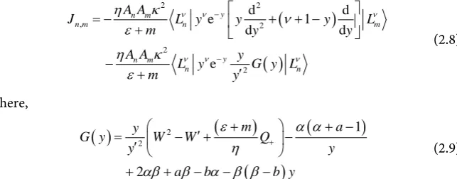
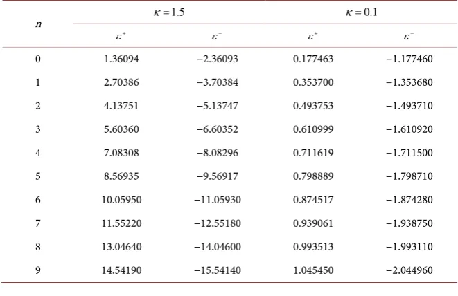
cannot be written in a closed form as the recursion relation cannot be compared to any well-known class of orthogonal polynomials contrary to what we had in the previous examples. In fact, the solutions are referred to new polynomials which have been called “dipole polynomials” and have been found in different physical problems like electron in the dipole field and non-central potential problems [19] [20], see also Equation (8) in [32]. Moreover, the eigenstates can be evaluated at any order and the energy eigenvalues can be computed numeri-cally with high accuracy. As an illustration, we have tabulated the lowest ten energy eigenvalues in Table 4. The spinor upper component for this system is written as

(

, n

)

j

( ) ( )

n j

j

x f x

ψ+ ε ₌

∑

ε φ+ _{, where}

{

( )

}

0

j n _j

f

ε

∞₌ are solutions to

(3.2.10) and

φ

j

( )

x

+ _{is written in terms of Jacobi basis below:}

( )

(

( )

)

2 1

(

( )

)

2 1 ( , )

(

( )

)

4 4

1 cos 1 cos cos

j x Aj x x Pj x

ν µ

µ ν

φ+ ₌ ₊ κ + ₋ κ + κ _(3.2.11)

where

(

1

) (

(

) (

)

2 1 1 1

1 1

2

n

n n n

A

n n

µ ν

κ

µ ν

ν

µ

+ +

+ + + Γ + Γ + + + =

Γ + + Γ + + . Similarly, we can fo-

llow this procedure to find solutions for the pseudo-spin-symmetric coupling for the same sinusoidal potentials. For more solvable potentials in the presence of spin symmetries, we have tabulated more results in Table 5.

3.3. General Case

An interesting example we mention here is when S=W =0, and V x

( )

=V x0 2, [image:13.595.208.539.522.736.2]

which can be used for an electron in graphene moving under the influence of a

Table 4. The first ten positive and negative energy solutions to Equation (3.23). Here we took m=1,V0=0.5, µ ν= =1 2, and κ=1.5, 0.1.

n κ =1.5 κ =0.1

ε+ _ε− _ε+ _ε−

(14)

[image:14.595.61.535.97.734.2]

DOI: 10.4236/jamp.2017.510172 2085 Journal of Applied Mathematics and Physics Table 5. Few examples of solvable potentials in the spin-symmetric coupling with the bound states spectrum formula and spinor wavefunction upper component for each [14]. One can obtain similar results in the pseudo-spin symmetry.

( )

V x =S x W x

( )

εn ψn

( )

x

+ 2 2 2 e e 2 x x

A λ B λ

λ _ − ₊ − _

  0 ( )

2

2 2 2 1

2

n n

A

m m n

B

ε − = −λ _ ε + + + _

  ( ) ( ) ( ) ( )

(

)

1 _e 2

2 ₂ ₁

e

2 e

x n

n

A _m _n _B B

n n

A _m _n

x B

n x A

L B m

λ λ ε ε _λ ψ ε − − + + + − + + + + − = × + m ε< , B>0,

(

1

) (

1

)

n

A = λΓ +n Γ + +n ν

0e

x

V −λ 0e

x

W −λ ( )

2

2 2 2 0

0

2 3

2

n n

V

m m n

W

ε λ ε

λ   − = − _ + + + _   ( ) ( ) ( )

(

)

0 0 0 0 0 2 3 e 2 4 2 3 0 e 2 e x V m n W W n n V m n W x n x A L W λ

λ ε λ

λ ε λ λ ψ λ − − + + + − + + + + − = × m

ε< , W0>0,

(

1

) (

1

)

n

A = λΓ +n Γ + +n ν

( )

0tanh

V=V λx W=W0tanh( )λx

2

2 2 2 2 2 2 2

0 0 2

n

n n n

m

m W V ε

ε λ ϑ ϑ

λ −   +   − = −  + _ _      1 2

n n D

ϑ =_ + − λ_

 

2 2 2

0 0 4

D =W +αW +λ

(

)

2

0 0 4

W W +α > −λ

( )

(

( )

)

(

( )

)

( )

(

( )

)

2 2

,

1 tanh 1 tanh tanh

n n

n

x A x x

P x

ν µ

µ ν

ψ λ λ

λ + ₌ ₊ ₋ ×

(

)

2 2 0 2

n n m V n m

µ = −_ε − − ε + _ λ

(

)

2 2 0

2

n n m V n m

ν = −_ε − + ε + _ λ

, 1

n n µ ν > −

(

)

2

e 1

e x 1 x

C A

λ

λ −

− ₋ + − 0

( )( )

2 2 2

2 2 1 2

1

4 2

2

n n

m A C

m n n ε λ λ ν ε _ν    + + −  = −  + + ₊   +     

( )2

2 2 2

1 4

n m

ε − = −λ µ+

( ) ( )( 1 2) ₍ ₎( 1 2) (,)_{( )}

1 1

n x An y y Pn y

ν µ µ ν

ψ + +

= − +

1 2e x

y= − −λ

(

)

₍ ₎

2 2

1

8 C n m

λ ν ε − = + ( ) ( )

(

)

( ) 2 2 0 1 2 sinh

2 tanh 1

2

cosh

V r

V V r

r λ λ λ + + −

+ 0 see [22] see [22]

( ) ( ) 0 1 2 tanh cosh

V V x

x

λ λ +

0 see [22] see [22]

( )

(

)

0 1 1 e 1 2 1 2e 1 e r r r V r V V V λ λ λ − + − = −   ×_ + + − _ −  

0 see [22] see [22]

( )

( ) ( )

( )

( ) ( )

2 0 2

2

2 1 2

1 4 2 1 1 2 1 1 V

V x V

x L x L

x L V

V

x L x L

+ −  =  + − _ −  + − − _ −

(15)

confining parabolic electrostatic barrier. Using the transformation

2 1 2

y=  κx_

 

in (2.11), we obtain

(

)

0 4

4 1

4

m V ε ρ

ηκ +

= − _{, and} 2 2

2

1 2

m ε ν

σ ηκ

− +

= + _forν = ±1 2.

The J-matrix for this situation is given below:

(

)

(

)

(

)

(

)

}

2 2 2

0

, 4 2 ,

0

, 1 , 1

4

8

1 1

2 2

4 1

( 1) 1

4

n m n m

m V m

J n

m

m V

n n n n

ε

ηκ ν ε _δ

ε ηκ ηκ

ε

ν δ ν δ

ηκ + −

 +  +  − 

  

= ₊ _ + _ + + 

   

 

 +

 _{ } _

− − _{ } + + + + + _

 

(3.3.1)

Using Equation (1.1), we write the three-term recursion relation as follows:

(

)

(

)

(

)

(

)

2 2

0

2 4

0

1 1

4

8

1 1

2 2

8

1 1

( 1) 1

2 2

n n

m V m

f n f

m V

n n f n n f

ε

ε ν

ηκ ηκ

ε

ν ν

ηκ − +

+

 

− _{= −} ₊ +  ₊

 

 _ 

+

 _{ } _

+ _ − _{ } + + + + + _

 

(3.3.2)

by comparison with the three-term recursion relation of Meixner-Pollaczek po-lynomials (A13), we find that the solutions to Equation (3.3.2) are the norma-lized Meixner-Pollaczek polynomials. Using the infinite spectrum formula of these polynomials (A13), we obtain the following bound states spectrum for

1 2

ν = _:

(

)

2 2

0 3 4

4

n n

m ε ε m η V n 

 − = ± − _ + _

  _ _ (3.3.3)

where ε >0,V0>0 (or ε <0,V0<0), and

4 0 32

m V

ε

> +

ηκ

_{. The upper}

spi-nor wavefunction associated with this case is given below:

(

)

2 2₈

( )

(

₂ ₂

)

, e 4

2

x

n j j n j

j

x κ x κ A f Lν x

ψ+ ε ₌ −

∑

ε κ _(3.3.4)

where

A

_j

= Γ +

(

j

1

) (

Γ +

j

3 2

)

,

( ) (

)

3 4 _;

n n

f = ω ξ P ξ θ , where

( )

3 4 _;

n

P ξ θ is

the Meixner-Pollaczek polynomial of order n in

ξ

,

ω ξ

( )

_{is its weight}

func-tion (A11), with

(

)

2 2

0 4

m

m V

ε ξ

ε η

− =

+ and

( )

(

)

0

(

)

0

4 4

8 1 8 1

cosh

2 2

m V m V

ε ε

θ

ηκ ηκ

+ +

   

=_ + _{ } − _

   

the spinor wavefunction lower component can be easily obtained using the above result in Equation (2.1).

We will not be able exhaust all solvable potentials in this section, but one can follow the same procedure to obtain different solvable potentials like

( )

0e

x V x =V −κ ,

( )

0sin

( )

V x =V

κ

x , and others. We should point out here that we have used the

(16)

ad-DOI: 10.4236/jamp.2017.510172 2087 Journal of Applied Mathematics and Physics

vised to refer to [23] and references therein.

4. Conclusion and Future Recommendations

We have solved the one-dimensional Dirac equation using the Tridiagonal Re-presentation Approach (TRA). This approach, even limited, provides a very easy and handy approach to find analytical solutions to a certain class of solvable tentials for the 1D Dirac Equation. In the presence of symmetry between the po-tential components in Dirac Equation, the problem can be reduced to solving an effective Schrodinger-like equation which was treated previously using the TRA

[15] [18] [19] [20] [21]. The solvable potential configurations we obtained have been discussed in details in Section 3. As a potential application of our analytical results, we have mentioned in Section 3 that some of our results can be used di-rectly in graphene to treat electrons subject to electrostatic or magneto static (or both) barriers, a subject of major importance in recent graphene literature. Fi-nally, we would like to express our interest in extending our approach to Dirac Equation in higher dimensions.

Acknowledgements

The authors would like to thank King Fahd University of Petroleum and Miner-als for their support under research group project RG1502-1 and RG1502-2. We also acknowledge the material support of the Saudi Center for Theoretical Phys-ics (SCTP). Our deep appreciation goes to Prof. Abdulaziz Alhaidari under whose guidance this research has been performed.

References

[1] Greiner, W. (1994) Relativistic Quantum Mechanics: Wave Equations. Springer, Berlin.

Bjorken, J.D. and Drell, S.D. (1964) Relativistic Quantum Mechanics. McGraw-Hill, New York.

[2] Dombey, N., Kennedy, P. and Calogeracos, A. (2000) Supercriticality and Trans-mission Resonances in the Dirac Equation. Physical Review Letters, 85, 1787.

https://doi.org/10.1103/PhysRevLett.85.1787

[3] Novoselov, K.S., Geim, A.K., Morozov, S.V., Jiang, D., Zhang, Y., Dubonos, S.V., Grigorieva, I.V. and Firsov, A.A. (2004) Electric Field Effect in Atomically Thin Carbon Films. Science, 306, 666.https://doi.org/10.1126/science.1102896

[4] Stander, N., Huard, B. and Goldhaber-Gordon, D. (2009) Evidence for Klein Tunneling in Graphene p-n Junctions. Physical Review Letters, 102, Article ID: 026807. https://doi.org/10.1103/PhysRevLett.102.026807

[5] Castro Neto, A.H., Guinea, F., Peres, N.M.R., Novoselov, K.S. and Geim, A.K. (2009) The Electronic Properties of Grapheme. Reviews of Modern Physics, 81, 109.

https://doi.org/10.1103/RevModPhys.81.109

Das Sarma, S., Adam, S., Hwang, E.H. and Rossi, E. (2011) Electronic Transport in Two-Dimensional Graphene. Reviews of Modern Physics, 83, 407.

https://doi.org/10.1103/RevModPhys.83.407

Geim, A. (2009) Graphene: Status and Prospects. Science, 324, 1530.

(17)

[6] Hartmann, R.R. and Portnoi, M.E. (2014) Quasi-Exact Solution to the Dirac Equa-tion for the Hyperbolic-Secant Potential. Physical Review A, 89, Article ID: 012101.

https://doi.org/10.1103/PhysRevA.89.012101

Eshghi, M. and Mehraban, H. (2017) Exact Solution of the Dirac-Weyl Equation in Graphene under Electric and Magnetic Fields. Comptes Rendus Physique, 18, 47.

https://doi.org/10.1016/j.crhy.2016.06.002

[7] Quesne, C. and Tkachuk, V.M. (2005) Dirac Oscillator with Nonzero Minimal Un-certainty in Position. Journal of Physics A, 38, 1747.

https://doi.org/10.1088/0305-4470/38/8/011

[8] Nouicer, K. (2006) An Exact Solution of the One-Dimensional Dirac Oscillator in the Presence of Minimal Lengths. Journal of Physics A, 39, 5125.

https://doi.org/10.1088/0305-4470/39/18/025

[9] Quesne, C. and Tkachuk, V.M. (2007) Generalized Deformed Commutation Rela-tions with Nonzero Minimal Uncertainties in Position and/or Momentum and Ap-plications to Quantum Mechanic. SIGMA, 3, 016.

[10] Jana, T.K. and Roy, P. (2009) Exact Solution of the Klein-Gordon Equation in the Presence of a Minimal Length. Physics Letters A, 373, 1239.

https://doi.org/10.1016/j.physleta.2009.02.007

[11] Witten, E. (2004) Supersymmetry and Other Scenarios. International Journal of Modern Physics A, 19, 1259. https://doi.org/10.1142/S0217751X04019160

Cooper, F., Khare, A. and Sukhatme, U. (2001) Supersymmetry in Quantum Me-chanics. World Scientific, Singapore. https://doi.org/10.1142/4687

[12] Yurov, A.V. (1997) Darboux Transformation for Dirac Equations with (1 + 1) Po-tentials. Physics Letters A, 225, 51. https://doi.org/10.1016/S0375-9601(96)00836-5

[13] Anderson, A. (1991) Intertwining of Exactly Solvable Dirac Equations with One-Dimensional Potentials. Physical Review A, 43, 4602.

https://doi.org/10.1103/PhysRevA.43.4602

Shishkin, G.V. (1993) On the Exact Description of the Dirac Particle in the Scalar and Pseudoscalar Fields. Journal of Physics A, 26, 4135.

https://doi.org/10.1088/0305-4470/26/16/029

[14] Alhaidari, A.D., Bahlouli, H. and Assi, I.A. (2016) Solving Dirac Equation Using the Tridiagonal Matrix Representation Approach. Physics Letters A, 380, 1577-1581.

[15] Alhaidari, A.D. (2005) An Extended Class of L 2-Series Solutions of the Wave Equa-tion. Annals of Physics, 317, 152-174. https://doi.org/10.1016/j.aop.2004.11.014

[16] Chihara, T.S. (2011) An Introduction to Orthogonal Polynomials. Courier Corpora-tion.

[17] Nikiforov, A.F. and Uvarov, V.B. (1988) Special Functions of Mathematical Physics. Vol. 205. Birkhäuser, Basel. https://doi.org/10.1007/978-1-4757-1595-8

[18] Alhaidari, A.D. (2005) Scattering and Bound States for a Class of Non-Central Po-tentials. Journal of Physics A, 38, 3409-3429.

https://doi.org/10.1088/0305-4470/38/15/012

[19] Alhaidari, A.D. and Bahlouli, H. (2008) Electron in the Field of a Molecule with an Electric Dipole Moment. Physical Review Letters, 100, Article ID: 110401.

[20] Alhaidari, A.D. and Ismail, M.E.H. (2015) Quantum Mechanics without Potential Function. Journal of Mathematical Physics, 56, Article ID: 072107.

https://doi.org/10.1063/1.4927262

(18)

I. The Infinite Potential Well with a Sinusoidal Bottom. Journal of Mathematical Physics, 49, Article ID: 082102. https://doi.org/10.1063/1.2963967

[22] Alhaidari, A.D. (2017) Solution of the Nonrelativistic Wave Equation in the Tridia-gonal Representation Approach. Journal of Mathematical Physics, 58, Article ID: 072104.

[23] Lewin, M. and Séré, É. (2014) Spurious Modes in Dirac Calculations and How to Avoid Them. In: Bach, V. and Delle Site, L., Eds., Many-Electron Approaches in Physics, Chemistry and Mathematics: A Multidisciplinary View, Mathematical Physics Studies IX, Springer, Berlin, 31-52.

https://doi.org/10.1007/978-3-319-06379-9_2

[24] Kuru, Ş., Negro, J. and Nieto, L.M. (2009) Exact Analytic Solutions for a Dirac Elec-tron Moving in Graphene under Magnetic Fields. Journal of Physics: Condensed Matter, 21, Article ID: 455305. https://doi.org/10.1088/0953-8984/21/45/455305

[25] De Martino, A., Dell’Anna, L. and Egger, R. (2007) Magnetic Confinement of Mass-less Dirac Fermions in Graphene. Physical Review Letters, 98, Article ID: 066802.

[26] Page, P.R., Goldman, T. and Ginocchio, J.N. (2001) Relativistic Symmetry Sup-presses Quark Spin-Orbit Splitting. Physical Review Letters, 86, 204.

[27] Arima, A., Harvey, M. and Shimizu, K. (1969) Pseudo LS Coupling and Pseudo SU 3 Coupling Schemes. Physics Letters B, 30, 517-522.

https://doi.org/10.1016/0370-2693(69)90443-2

[28] Hecht, K.T. and Adler, A. (1969) Generalized Seniority for Favored J≠ 0 Pairs in Mixed Configurations. Nuclear Physics A, 137, 129-143.

https://doi.org/10.1016/0375-9474(69)90077-3

[29] Ginocchio, J.N. (1999) A Relativistic Symmetry in Nuclei. Physics Reports, 315, 231-240. https://doi.org/10.1016/S0370-1573(99)00021-6

[30] De Castro, A.S., et al. (2006) Relating Pseudospin and Spin Symmetries through Charge Conjugation and Chiral Transformations: The Case of the Relativistic Har-monic Oscillator. Physical Review C, 73, Article ID: 054309.

https://doi.org/10.1103/PhysRevC.73.054309

[31] Akcay, H. (2009) Dirac Equation with Scalar and Vector Quadratic Potentials and Coulomb-Like Tensor Potential. Physics Letters A, 373, 616-620.

[32] Alhaidari, A.D. (2017) Orthogonal Polynomials Inspired by the Tridiagonal Repre-sentation Approach. arXiv:1703.04039 [math-ph]

(19)

Appendix A: Orthogonal Polynomials

A1. The Generalized Laguerre Polynomials:

Theses polynomials are solutions of the following second order differential equation:

(

)

( )

2

d d

1 0

d

d n

y y n L y

y y

ν

 

+ + − + =

 

  (A1)

where y∈ ∞

[ [

0, , ν > −1, and n∈Z+.

These polynomials satisfy the following useful properties:

( )

(

)

1

( )

d

( )

d n n n

y L y nL y n L y

y

ν ν _ν ν

−

= − + _(A2)

( ) (

2 1

) ( ) (

)

1

( ) (

1

)

1

( )

n n n n

yLν y = n+ +

ν

Lν y − +n

ν

Lν₋ y − +n Lν₊ y (A3)

( ) ( )

(

)

,

0

1

e d

!

y

n m n m

n

y L y L y y

n

ν ν ν ν _δ

∞

− ₌Γ + +

∫

(A4)

A2. The Jacobi Polynomials: Jacobi polynomials ( , )

( )

n

Pµ ν y defined on

[ ]

−1,1 are solutions to the

follow-ing ODE:

(

2

)

2

(

)

(

)

( , )

( )

2

d d

1 2 1 0

d

d n

y y n n