Munich Personal RePEc Archive
Rational Inattention and the Dynamics
of Consumption and Wealth in General
Equilibrium
Luo, Yulei and Nie, Jun and Wang, Gaowang and Young,
Eric
18 April 2017
Rational Inattention and the Dynamics of Consumption and Wealth in
General Equilibrium
∗
Yulei Luo†
University of Hong Kong
Jun Nie‡
Federal Reserve Bank of Kansas City
Gaowang Wang§
Shandong University
Eric R. Young¶ University of Virginia
April 18, 2017
Abstract
We use a recursive utility version of a basic Huggett (1993) model to study the cross-sectional dispersion of consumption and wealth (relative to income). The basic model implies too little dispersion compared to the data, whereas a one-parameter extension to include rational inatten-tion (limited informainatten-tion processing) delivers a better fit to both facts in general equilibrium. In particular, intertemporal substitution plays an important role in determining the two key dispersion moments via affecting the degree of optimal attention in equilibrium. Alternative models that rely on habit formation, incomplete information about current income, or borrow-ing constraints are not consistent with the facts we document.
Keywords:Rational Inattention; General Equilibrium; Consumption and Wealth Volatility.
JEL Classification Numbers:C61; D83; E21.
∗We are grateful to Laura Veldkamp (editor) and two anonymous referees for many constructive suggestions and
comments. We also would like to thank Ken Kasa, Chris Sims, Neng Wang, Mirko Wiederholt, and Christian Zimmer-mann for helpful discussions and suggestions, and conference and seminar participants in the 2015 SED annual meeting, the 11th world congress of the econometric society, the 2015 international conference on computing in economics and finance, University of Kansas, Kansas City Fed, University of Hong Kong, Central University of Finance and Economics and Shandong University for helpful comments. Luo thanks the General Research Fund (GRF No. HKU791913) in Hong Kong for financial support. We thank Andrew Palmer for excellent research assistance. All errors are the responsibility of the authors. The views expressed here are the opinions of the authors only and do not necessarily represent those of the Federal Reserve Bank of Kansas City or the Federal Reserve System. All remaining errors are our responsibility.
†Faculty of Business and Economics, The University of Hong Kong, Hong Kong. E-mail:[email protected]. ‡Research Department, Federal Reserve Bank of Kansas City. E-mail:[email protected].
1. Introduction
Our interest in this paper is to evaluate the general equilibrium implications of limited
information-processing capacity (rational inattention or RI) for the joint cross-sectional dispersions of consump-tion, wealth, and income. The evolution of the consumpconsump-tion, income, and wealth inequality based on optimal consumption-saving choice is a central topic in modern macroeconomics. In
intertem-poral consumption-savings problems,prudenthouseholds save today for three reasons: (i) they
an-ticipate future declines in income (saving for a rainy day), (ii) they face uninsurable risks
(precau-tionary savings), and (iii) they are patient relative to the interest rate. For example, the “permanent income hypothesis” (PIH) of Friedman (1957) emphasizes the motive (i) in which consumption is
solely determined by permanent income (the annuity value of total wealth) and follows a random
walk (see Hall 1978).1
A growing recent literature inspired by Sims (2003) shows that RI plays an important role in influencing the consumption and saving dynamics and has also gained some empirical support. Specifically, Sims (2003), Luo (2008), and Luo and Young (2010) introduce RI into the basic partial
equilibrium PIH environment; RI implies that agents process signals slowly and therefore appear to respond sluggishly to innovations in permanent income. This sluggish response appears to
deliver changes in consumption in response to anticipated income changes, and as a result also delivers smaller responses to permanent income changes; that is, the model delivers both excess
sensitivity and excess smoothness in the consumption behavior we observed in the US data.2 Some
empirical studies found that incomplete information about the state plays an important role in
af-fecting individual agents’ optimal decisions. For example, Coibion and Gorodnichenko (2015) and Andrade and Le Bihan (2013) find pervasive evidence consistent with Sims (2003)’s rational
inat-tention theory using the U.S. and European surveys of professional forecasters and other agents,
respectively.3 Crucial for our purposes, the RI model delivers only one new free parameter, which
maps directly into the speed of learning (one can think of this parameter as a filter gain).
However, the above RI-PIH models are partial equilibrium, taking as given a constant exoge-nous risk-free rate. By construction, the models shut off the feedback loop from the equilibrium
1This statement holds, for example, if households have quadratic utility and have access to a single risk-free bond
with a constant return. If utility is not quadratic, the random walk nature of consumption is only approximately true, but the PIH still holds.
2The tests of the PIH, while robust to the possibility that agents have more information than the econometrician (see
Campbell and Deaton 1989), may not be robust to the RI implication that the econometrician may actually have more information than the agents (at least at the time of decisions). The reason is that agents with more information will still set consumption changes to be orthogonal to everything the econometrician observes; it is clear that the converse would not necessarily hold.
3Hong, Torous, and Valkanov (2007) find evidence for rational inattention in the financial markets. Specifically,
interest rate to the dynamics of consumption and wealth. Furthermore, these RI models do not sep-arate risk aversion from intertemporal substitution in determining consumption dynamics, while many papers on recursive utility (RU) preferences highlight the importance of the separation
be-tween risk aversion and intertemporal substitution in affecting optimal consumption-portfolio rule and asset pricing. (See, for example, Epstein and Zin 1989, Campbell 2003, Vissing-Jï¿œrgensen
and Attanasio 2003, Guvenen 2006.) This paper therefore fills the gap by providing a general theo-retical RU framework to explore the general equilibrium implications of rational inattention for the
joint cross-sectional dispersion of consumption, wealth and income. We investigate both the theo-retical mechanism (how RI influences the equilibrium interest rate) and the empirical performance
(how RI could lead the model to fit the data better compared to alternative hypotheses).
Specifically, we propose an equilibrium precautionary saving model in which inattentive con-sumers have recursive utility with exponential risk and intertemporal attitudes and face
uninsur-able labor income. We disentangle two distinct aspects of preferences: the agent’s elasticity of intertemporal substitution (EIS; attitudes towards variation in consumption across time) with the
coefficient of absolute risk aversion (CARA; attitudes towards variation in consumption across
states).4 We solve our model in closed-form and analytically inspect how risk aversion and
in-tertemporal substitution interact with rational inattention and then affect the equilibrium interest rate as well as the cross-sectional dispersion of consumption and wealth (relative to income). We
find that if attention is elastic (i.e., consumers can adjust the degree of attention in response to changes in the real world), the EIS plays an important role in affecting the equilibrium properties
of the model economy.5 In particular, we show that an increase in EIS affects the equilibrium
in-terest rate through two channels: (i) it increases the relative importance of the impatience-induced
dissaving effect (the direct channel) and (ii) it reduces the optimal attention level and thus increases
the inattention-induced precautionary saving amount (the indirect channel). In addition, the
opti-mal level of attention in our RU model is mainly determined by the EIS, and is independent of the
degree of risk aversion. We also show that the general equilibrium exists and is unique in such an RI-RU economy.
We then bring the theory to the data as well as compare with alternative hypotheses to
ex-4Constant-relative-risk-aversion (CRRA) utility functions are more common in macroeconomics, mainly due to
balanced-growth requirements. CRRA utility would greatly complicate our analysis because the intertemporal sumption model with CRRA utility and stochastic labor income has no explicit solution and leads to non-linear con-sumption rules. Introducing RI would then be substantially more difficult and involve approximations of unknown quality.
5Coibion and Gorodnichenko (2015) find that information rigidities were falling from the late 1960s to the early 1980s
amine whether our RI model can better explain the data. We use the RI model to interpret the
dispersion of consumption and wealth (relative to income) that we observe in the data.6 We find
that RI substantially improves the predictions of the model for these relative dispersions. The
full-information model, for the income process we estimate from micro data, implies that these dispersions are much lower than in the data; the separation of risk aversion and intertemporal
substitution made feasible by recursive utility does not help increase these dispersions. For plau-sible value of the CARA and EIS, the dispersion of consumption and wealth relative to income is
still well below their empirical counterparts. With RI, as households become less attentive, relative dispersions in consumption and wealth both rise. Interestingly, we find that the same value of
the RI parameter roughly matches both moments, providing an over-identifying test of the model. General equilibrium effects turn out to be less significant when consumers are less
information-constrained, acting to slightly reduce the dispersions in the model relative to a partial equilibrium exercise with a fixed interest rate.
Next, we ask whether our model provides a story for the observed changes in the
cross-sectional distributions of consumption and income. The significant increase in household income inequality or dispersion for the U.S. in the 1980s and 1990s is a well-documented fact. Many
stud-ies have found that the dispersions of U.S. household earnings and incomes have a strong upward
trend.7 In addition, the literature has documented that the recent increase in income inequality
in the U.S. has not been accompanied by a corresponding rise in consumption inequality over the 1980s and 1990s. In other words, over the sampling period income and consumption inequality
diverged and the relative volatility of consumption to income has decreased, as discussed Krueger and Perri (2006) and Blundell, Pistaferri, and Preston (2008). With elastic attention we find that our model naturally predicts a decline in the relative volatility of consumption to income, in response
to a rise in income volatility, and the magnitude is close to that found in our data; this experiment provides additional evidence for our model.
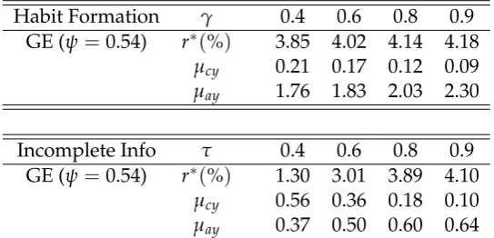
To further justify the validation of RI in explaining the data, we compare our RI model with several alternative models that are commonly used to study consumption dynamics in the
litera-ture. We first compare our RI model with models of sluggish movements in consumption, namely habit formation and incomplete information about current income. As the habit parameter
in-creases, consumption changes become sluggish as households try to smooth changes in
consump-6As the PSID does not have complete consumption information, we construct a panel with consumption and income
based on the approach from Guvenen and Smith (2014) to impute total consumption via a demand system estimated on the CEX (see also Blundell, Pistaferri, and Preston 2008). We also use the PSID to construct measures of wealth, and then we compare our measures to those predicted by the model.
7See Katz and Autor (1999) for a survey of these empirical findings. Table 1 also reports the increases in the variance
tion rather than levels. Thus, there is a sense in which the two model frameworks look similar; in fact, Luo (2008) shows that the two models are observationally equivalent at the aggregate level (in terms of consumption growth dynamics), but not at the individual level: RI delivers high
con-sumption volatility from the noise shocks. We show that this similarity does not extend to the equilibrium cross-sectional dispersion moments we examine here, even though the noise shocks
aggregate out; unlike RI, habit formation moves the relative dispersion of consumption to income away from its empirical counterpart, and the model’s prediction on the wealth dispersion is well
below its empirical counterpart.8 In addition, we find that stronger habit formation leads to higher,
not lower, interest rates.
With incomplete information, households cannot distinguish between permanent and transi-tory innovations in current income; although similar to rational inattention on its face, there is a key difference – under RI, agents cannot observe the value of their assets in addition to their
in-come, and therefore need to extract endogenous as well as exogenous components. It turns out that incomplete information economies behave very much like habit models – the larger the MA
coefficient on the forecast of future income (which captures the speed of learning), the higher the equilibrium interest rate. Consequently, the consumption dispersion measure gets too small, and
the wealth dispersion measure remains far too low.
Finally, we consider whether introducing borrowing constraints can deliver the observed
dis-persion measures. We argue that they cannot, based on an additional observation – we find that our relative dispersion measure for consumption does not vary across the income and wealth
dis-tributions. In models that rely mainly on borrowing constraints, households near the constraint have high marginal propensities to consume, which leads them to respond very strongly to income changes; as a result, the relative variation in consumption for “poor” households is much higher
than that for “rich” ones. Given that this difference is decisively rejected by the data we conclude that borrowing constraints are not a critical ingredient in a model of cross-sectional consumption,
income, and wealth dynamics.
This paper is organized as follows. Section 2 constructs a precautionary saving model with
a continuum of inattentive consumers who have the recursive utility and face uninsurable labor income. Section 3 solves optimal consumption-saving rules under rational inattention and
char-acterizes the unique general equilibrium of this economy. Section 4 examines how RI affects the interest rate and the joint dynamics of consumption, income, and wealth quantitatively. Section 5 compares the rational inattention model to the models with habit formation, incomplete
infor-8Relative wealth dispersion is not strictly monotone in the habit parameter, but the change occurs at very high habit
mation about current income, and borrowing constraints. In the appendices we provide the key proofs and derivations.
2. A Caballero-Huggett-Wang Economy with Rational Inattention
2.1. A Full-information Rational Expectations Model with Recursive Utility and
Precautionary Savings
In this section, we first consider a full-information rational expectations (FI-RE) recursive
util-ity model with labor income and precautionary savings. Although the expected utilutil-ity model has many attractive features, it implies that the agent’s elasticity of intertemporal substitution is
the reciprocal of the coefficient of relative risk aversion. However, risk aversion (attitudes to-wards atemporal risks) and intertemporal substitution (attitudes toto-wards shifts in consumption
over time) capture two distinct aspects of preferences, and should not necessarily be linked so
tightly.9 In this paper, we assume that agents in our model economy have recursive preferences of
the Kreps-Porteus/Epstein-Zin type, and can disentangle the degree of risk aversion from the
elas-ticity of intertemporal substitution. Specifically, for every stochastic consumption stream,{ct}∞t=0,
the utility stream,{f(Ut)}∞t=0, is recursively defined as follows:10
f(Ut) = f(ct) + 1
1+ρf(CEt[Ut+1]) (1)
whereρ>0 is the agent’s subjective discount rate, f(x) =−ψexp(−x/ψ),
CEt[Ut+1] =g−1(Et[g(Ut+1)]), (2)
is the certainty equivalent ofUt+1conditional on the periodtinformation, andg(Ut+1) =−exp(−αUt+1)/α.
In (1),ψ>0 governs the elasticity of intertemporal substitution (EIS), whileα>0 governs the
co-efficient of absolute risk aversion (CARA). Ifψ= 1/α, the functions f andgare the same and the
recursive utility reduces to the standard time-separable expected utility function used in Caballero
(1990) and Wang (2003). In addition,ψ = 1/αalso implies that the consumer is indifferent about
the time at which uncertainty is resolved.11
9Risk aversion describes the agent’s reluctance to permit consumption to vary across different states of the world
and is meaningful even in a static setting. In contrast, intertemporal substitution describes the agent’s willingness to substitute consumption over time and is meaningful even in a deterministic setting. Furthermore, many estimates in the literature reject the special case of expected utility.
10Angeletos and Calvet (2006) adopt similar recursive utility preferences to study the effects of idiosyncratic
produc-tion risks on business cycles and growth.
11Consumers prefer early resolution of uncertainty ifα>1/ψand late resolution ifα<1/ψ. Luo and Young (2016)
Following Caballero (1990) and Wang (2003), the flow budget constraint is written as
at+1= (1+r)at+yt−ct, (3)
whereris a constant rate of interest and labor income,yt, follows a stationary AR(1)process with
Gaussian innovations
yt= φ0+φ1yt−1+wt, t≥1, |φ1|<1, (4)
wherewt ∼ N 0,σ2,φ0 = (1−φ1)y,yis the mean ofyt, and the initial levels of labor incomey0
and asseta0are given.12
In order to facilitate the introduction of rational inattention, we follow Luo (2008) and Luo and
Young (2010) and reduce the multivariate model to a univariate model with iid innovations to total
wealth. Let total wealth,st =at+ht, be defined as a new state variable. Here
ht≡ 1
1+rEt
"∞
∑
j=0
1
1+r
j
yt+j
#
, (5)
is human wealth (defined as the discounted expected present value of current and future labor income); evaluating the sum yields
ht =φ
yt+ φ0
r
,
whereφ = 1/(1+r−φ1).13 Using (3) and (4), it is straightforward to show that the evolution of
the new state variable can be written as
st+1= (1+r)st−ct+ζt+1, (6)
where the time(t+1)innovation to total wealth can be written as
ζt+1 ≡ 1
1+r
∞
∑
j=t+1
1
1+r
j−(t+1)
(Et+1−Et)yj, (7)
which can be reduced toζt+1 =φwt+1if we use income process (4).14
12Assuming that the individual income shock includes two components, one permanent and the other transitory,
does not change the main results in this paper. Here we follow Wang (2003) and adopt specification (4), in order to simplify the algebra. A detailed derivation of the model with the two-income shock specification is available from the corresponding author by request. For the empirical studies on the income specification, see Attanasio and Pavoni (2011).
2.2. Incorporating Rational Inattention
In this section, we follow Sims (2003) and incorporate rational inattention (RI) due to finite
information-processing capacity into the above permanent income model with the CARA-Gaussian specifica-tion. Under RI, consumers have only finite Shannon channel capacity available to observe the
state of the world. Specifically, we use the concept of entropy from information theory to charac-terize the uncertainty about a random variable; the reduction in entropy is thus a natural measure
of information flow. With finite capacityκ ∈ (0,∞), a random variable{st}following a
contin-uous distribution cannot be observed without error and thus the information set at time t+1,
denotedIt+1, is generated by the entire history of noisy signals
n
s∗jot+1
j=0. Following the literature,
we first assume the noisy signal takes the additive form:15
s∗t+1 =st+1+et+1,
whereet+1is the endogenous noise caused by finite capacity.16 We further assume thatet+1is an iid
idiosyncratic shock and is independent of the fundamental shocks hitting the economy. The reason
that the RI-induced noise is idiosyncratic is that the endogenous noise arises from the consumer’s own internal information-processing constraint. Agents with finite capacity will choose a new
signals∗t+1∈ It+1 =
s∗1,s2∗,· · ·,s∗t+1 that reduces the uncertainty about the variablest+1as much
as possible. Formally, this idea can be described by the information constraint
H(st+1|It)− H(st+1|It+1)≤κ, (8)
whereκis the investor’s information channel capacity,H(st+1| It)denotes the entropy of the state
prior to observing the new signal att+1, andH(st+1| It+1)is the entropy after observing the new
signal. κimposes an upper bound on the amount of information flow – that is, the change in the
entropy – that can be transmitted in any given period. Finally, following the literature, we suppose
that the prior distribution ofst+1is Gaussian.
In a linear-quadratic-Gaussian (LQG) setting, Sims (2003) and Shafieepoorfard and Raginsky
(2013) show thatex postGaussian distributions, st|It ∼ N(E[st|It],Σt)withΣt = Et
h
(st−bst)2
i
,
15Mackowiak and Wiederholt (2009) show that this additive noisy signal form is optimal if the state being tracked is a
stationary Gaussian AR(1) process. The proof for the optimal form of the noisy signal in their paper can be extended to our model in which the state being tracked is a random walk if the channel capacity,κ, is greater than a lower bound so that all conditional moments appearing in the proof are finite and well-defined. Please see the proof in Online Appendix A for the details.
16For other types of imperfect information about state variables, see Pischke (1995) and Wang (2004). Pischke (1995)
are optimal. Here we first assumeex post Gaussian distributions of the true state and Gaussian noise but adopt negative exponential recursive utility preferences. Because both the optimality ofex postGaussianity and the standard Kalman filter are based on the linear-quadratic-Gaussian
(LQG) specification, the applications of these results in the RI models with negative exponential
preferences are only approximately valid.17 In the next section we verify that the loss function due
to RI is approximately quadratic and consequently the optimality of theex postGaussianity of the
state approximately holds in the recursive utility model.
Since bothex anteandex postdistributions of the state are Gaussian, (8) reduces to
ln(|Ψt|)−ln(|Σt+1|)≤2κ, (9)
whereΣt+1 = vart+1(st+1)andΨt = vart(st+1) = (1+r)2Σt+vart(ζt+1)are the posterior and
prior variances of the state variable,st+1, respectively. In our univariate model, (9) fully determines
the value of the steady state conditional varianceΣ:
Σ= vart(ζt+1)
exp(2κ)−(1+r)2, (10)
which means thatΣ is entirely determined by the variance of the exogenous shock (vart(ζt+1))
and finite capacity(κ). To guarantee that the state is stabilizable and the unconditional variance
converges, we need to make the following assumption on the amount of channel capacity:
Assumption 1
κ >ln(1+r). (11)
It is worth noting that this restriction is very weak ifr is small; in general equilibriumr will be
smaller thanρ, so for short time periods this condition is not restrictive at all.
Following the steps outlined in Luo and Young (2014), we can compute the Kalman gain in the
steady stateθas
θ =1−exp1(2κ); (12)
θmeasures the fraction of uncertainty removed by a new signal in each period, and is the only new
parameter introduced by the rational inattention framework.
The evolution of the estimated statebstis governed by the Kalman filtering equation
bst+1= (1−θ) ((1+r)bst−ct) +θs∗t+1, (13) 17See Peng (2004), Mondria (2010), and Van Nieuwerburgh and Veldkamp (2009, 2010) for applications of CARA
wherebst= Et[st]is the conditional mean of the state,st. Combining (6) with (13) yields
bst+1= (1+r)bst−ct+ζbt+1, (14)
where
b
ζt+1= θ(1+r) (st−sbt) +θ(ζt+1+et+1) (15)
is the innovation tobst+1 and is independent of all the other terms on the RHS of (14). ζbt+1 is an
MA(∞)process withEt
h b
ζt+1 i
=0 and
varζbt+1
=Γ(θ,r)ω2ζ, (16)
whereωζ2=vart(ζt+1),
Γ(θ,r) = θ
1−(1−θ) (1+r)2
>1 (17)
forθ<1, and
st−bst=
(1−θ)ζt
1−(1−θ) (1+r)·L−
θet
1−(1−θ) (1+r)·L (18)
is the estimation error withEt[st−bst] =0 and var(st−bst) = 1−(1−1−θ)(θ1+r)2ωζ2;Lis the standard lag
operator. To guarantee that the sum of these infinite series converges, we impose the restriction
κ>0.5 ln(1+r), which is weaker than (11). From (17), it is clear that ∂Γ
∂r >0 and ∂
Γ
∂θ <0.
3. General Equilibrium under RI
3.1. Optimal Consumption and Savings Functions
The consumption function and the value function under RU and RI can be obtained by solving the Bellman equation:
f(J(bst)) =max ct
f(ct) + 1
1+ρf(CEt[J(bst+1)])
, (19)
subject to (14)-(18). The following proposition summarizes the main results from the above precautionary-savings model with RI.
Proposition 1. For a given Kalman gain,θ, the value function is
b
v(bst) =−ψ
r exp
−ψ1
rbst−ψln(1+r) +
ψ r ln
1+ρ
1+r
− 12αrω2ζb
, (20)
the consumption function is
c∗t =rbst+ψ
and the saving function is
d∗t = eft+r(st−bst) +Π(θ,r)− ψ
rΨ(r), (22)
where eft ≡ (1−φ1)φ(yt−y)captures the consumer’s demand for savings “for a rainy day”,bst
is governed by (14), st−bst is an MA(∞)estimation error process given in (18), Π(θ,r) ≡ αrω2bζ/2 =
rαΓ(θ,r)ω2ζ/2 is the precautionary saving demand, and Ψ(r) ≡ ln11++ρr captures the
patience-induced saving.
Proof. See Appendix 7.1 for the derivations.
Given the value function (20), we can show that the loss function due to RI is approximately quadratic and the optimality of the ex post Gaussianity of the state still approximately holds in the
RU model, which justifies the Kalman filtering equation, (14). See Appendix 7.2 for the detailed proof.
Asκ converges to ∞ (or θ converges to 1), bst and ω2
b
ζ reduce tobst andω
2
ζ, respectively;
con-sequently, our RI model reduces to the full-information rational expectations (FI-RE) model.18 To
explore the effects of limited attention on precautionary savings within the RU framework, we first define the precautionary saving premium due to limited attention as
Pri ≡ 1
2(Γ(θ,r)−1)αrω
2
ζ, (23)
whereΓ(θ,r)is given in (17). It is clear that this premium is decreasing with the degree of
atten-tionθ, and is increasing with the coefficient of absolute risk aversion(α)and the persistence and
volatility of the income shock (φ1andσ) for any givenθ. Thus, the incomplete information that RI
forces upon the households leads to an increase in saving.
To further explore the precautionary savings premium in (23), we isolate the effects of RI on individual consumption and saving by rewriting (21) as
c∗t =rbst+
ψ
rΨ(r)− 1 rα
ln(Et[exp(−rαθ(1+r) (st−bst))]) +12 rαθωζ 2
+ 1
2(1−θ)Γ(θ,r) rαωζ 2
, (24)
whereΨ(r) =ln11++ρrmeasures the relative importance of patience to the interest rate in
deter-mining optimal consumption (it is greater than 0 ifρ >r),
1
αrln(Et[exp(−αrθ(1+r) (st−bst))]) = 1
2rαθ(1−θ)Γ(θ,r) (1+r)
2
ω2ζ
is the precautionary savings premium due to the timet estimation error, rαθωζ 2
/2 is the
pre-cautionary savings premium driven by the exogenous fundamental income shocks {wt}, and
(1−θ)Γ(θ) rαωζ 2
/2 captures the precautionary savings premium driven by the endogenous
noise shocks, {et}.19 From (21), for finite capacity (κ < ∞ or θ ∈ (0, 1)), the precautionary
saving premium due to fundamental shocks is smaller than that in the full-information case,
rαθωζ 2
/2 < rαωζ2/2, because of the incomplete adjustment of consumption to the
funda-mental shock; however, we have two new positive terms that increase the total savings more than
the absolute value of the reduced savings: (i) the premium due to the estimation error and (ii) the premium due to the RI-induced endogenous noise.
Given the timetavailable information and the fact thatEt[st−bst] =0, the conditional mean of
(22) can be written as
e
dt= eft+Π(θ,r)−ψ
rΨ(r). (25)
3.2. Existence and Uniqueness of General Equilibrium
As in Wang (2003), we assume that the economy is populated by a continuum ofex anteidentical,
but ex postheterogeneous agents, of total mass normalized to one, with each agent solving the optimal consumption and savings problem with RI specified in (19). Similar to Huggett (1993), we
also make the following assumption:
Assumption 2The risk-free asset in our model is a pure-consumption loan and is in zero net supply.
The initial cross-sectional distribution of permanent income is a stationary distributionΦ(·).
By the law of large numbers in Sun (2006), provided that the spaces of agents and the prob-ability space are constructed appropriately, aggregate permanent income and the cross-sectional
distribution of permanent incomeΦ(·)are constant over time.
Proposition 2. The total savings demand “for a rainy day” in the precautionary savings model with RI
equals zero for any positive interest rate. That is, Ft(r) =´yt eft(r)dΦ(yt) =0, for r>0.
Proof. The proof uses the LLN and is the same as that in Wang (2003).
Proposition 2 states that the total savings “for a rainy day” is zero, at any positive interest rate.
Therefore, from (22), forr>0, the expression for total savings under RI in the economy at timetis
D(θ,r)≡Π(θ,r)−ψ
rΨ(r), (26)
19This result is derived by using Equation (18) and the iid property of the processesnζb t o
whereΠ(θ,r) =rαΓ(θ,r)ωζ2/2 measures the amount of precautionary savings, andΨ(r)captures the patience-induced saving effect. Given (26), an equilibrium under RI is defined by an interest
rater∗ satisfying
D(θ,r∗) =0. (27)
The following proposition shows the existence of the equilibrium and the PIH holds in the RI general equilibrium.
Proposition 3. There exists a unique equilibrium with an interest rate r∗ ∈ (0,ρ)in the precautionary-savings model with RI. In equilibrium, each agent’s consumption is described by the PIH, in that
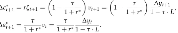
c∗t =r∗bst, (28)
wherebst = E[st|It] is the perceived value of permanent income. The evolution equations of wealth and
consumption are
∆c∗t+1 =r∗ζbt+1, (29)
∆a∗t+1 = 1−φ1
1+r∗−φ1 (yt−y) +r∗(st−bst), (30)
respectively, whereζbt+1is specified in (15) with Et
h b
ζt+1 i
=0,varζbt+1
=Γ(θ,r∗)ωζ2, andΓ(θ,r∗) = θ
1−(1−θ)(1+r∗)2. In the general equilibrium, the value function under RI can be written as
b
v(bst) =−ψ(1+r)
r exp
−ψrbst
, (31)
Proof. Ifr >ρ, the two terms,Π(θ,r)and−ψΨ(r)/r, in the expression for total savingsD(θ,r∗),
are positive, which contradicts the equilibrium condition,D(θ,r∗) =0. SinceΠ(θ,r)−ψΨ(r)/r <
0 (> 0) when r = 0 (r = ρ), the continuity of the expression for total savings implies that there
exists at least one interest rater∗ ∈ (0,ρ) such that D(θ,r∗) = 0. From (21), we can obtain the
individual’s optimal consumption rule under RI in general equilibrium asc∗t = r∗bst. Substituting
(14) and (28), we can obtain (29). (28) into (3) yields (30). The proof of uniqueness is longer and relegated to Appendix 7.3.
The intuition behind Proposition 3 is similar to that in Wang (2003). With an individual’s
con-stant total precautionary savings demandΠ(θ,r), for anyr > 0, the equilibrium interest rater∗
must be such that each individual’s dissavings demand due to impatience is exactly balanced by
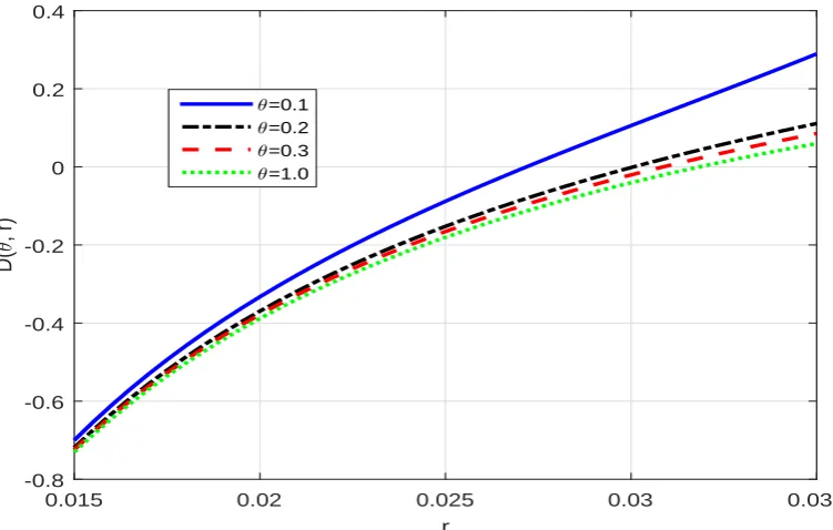
as a function ofθ, given the parametersα=2,ψ=0.54,φ1= 0.92,σ= 0.175, andρ= 0.04.20 It is
clear from the figure that the equilibrium interest rate increases withθ.
Regarding uniqueness, Toda (2017) demonstrates that the FI-RE model used here can have
multiple stationary equilibria, provided the income process is sufficiently rich; the AR(1) process we use here does not satisfy the requirements for multiple equilibria, though. Our results suggest
that RI does not deliver any new insights into the nature of multiple equilibria, so we do not investigate this issue further.
The magnitude of the EIS(ψ)is a key issue in macroeconomics and asset pricing. For example,
Parker (2002) and Vissing-Jorgensen and Attanasio (2003) estimate the IES to be well in excess of
one. Hall (1988) and Campbell (2003), on the other hand, estimate its value to be well below one.
Here we chooseψ = 0.5 for illustrative purposes and will examine how EIS affects the general
equilibrium under RI in Section 4 when we do the quantitative analysis.21 From the equilibrium
condition (27), it is clear that a high value ofψwould amplify the relative importance of the
dissav-ing effectΨ(r)for the equilibrium interest rate. The intuition behind this result is simple. When
ψis higher, consumption growth responds less to changes in the interest rate. In order to clear the
market, the consumer must be offered a higher equilibrium risk free rate in order to be induced
to save more and making his consumption tomorrow even more in excess of what it is today (less smoothing).
Given (21) and (27), it is clear that even though the individual increases their total precautionary
savings in response to information frictions for a givenr, the level of aggregate savings equals zero.
That is, RI does not affect the aggregate wealth in the economy, because the equilibrium interest
rate is pushed down to counteract this precautionary savings increase.22 With lower Shannon
channel capacity, the equilibrium interest rate is lower.
From the equilibrium condition,
1 2r
∗αΓ(θ,r∗)ω2 ζ −
ψ r∗ ln
1+ρ
1+r∗
=0, (32)
20In Section 4.1, we will provide more details about how we estimate the income process using the U.S. data. The
main result here is robust to the choices of these parameter values.
21Guvenen (2006) finds that stockholders have a higher EIS (around 1.0) than non-stockholders (around 0.1). Crump,
Eusepi, Tambalotti, and Topa (2015) find that the EIS is precisely and robustly estimated to be around 0.8 in the general population using the newly released FRBNY Survey of Consumer Expectations (SCE).
22If we introduced an asset with elastic supply, such as the capital stock in Aiyagari (1994), the same effects would be
it is straightforward to show that
dr∗ dθ =
r∗3(2+r∗) h
1−(1−θ) (1+r∗)2i2
2r∗θ[1−(1−θ) (1+r∗)]
h
1−(1−θ) (1+r∗)2i2 +
2ψ
α(1+r∗)ω2 ζ
−1
. (33)
where 1−(1−θ) (1+r∗)2>0. It is clear from this expression thatr∗is decreasing in the degree of
inattention 1−θ. The first row of Table 2 reports the general equilibrium interest rates for different
values ofθ.23We can see from the table thatr∗decreases as the degree of inattention increases. For
example, ifθ is reduced from 1 to 0.1,r∗is reduced from 3.41 percent to 2.89 percent. In addition,
it is clear that
dr∗
dα <0 and
dr∗ dψ >0.
That is, the equilibrium interest rate decreases with the degree of risk aversion and increases with the degree of intertemporal substitution. Here it is worth noting that although both the CARA
model and the LQ model lead to the PIH in general equilibrium, both risk aversion and intertem-poral substitution play roles in affecting the dynamics of consumption and wealth in the CARA
model via the equilibrium interest rate channel.
One might ask what a reasonable value of θ is, and if there is any way to calibrate it outside
a model. Unfortunately, there is no direct survey evidence on the value of channel capacity of or-dinary households in the economics literature, and thus it is not straightforward to answer these
questions; estimates of learning capacity exist, but they are not directly useful since we are in-terested in the capacity that will be devoted to economic activity (specifically, consumption and
saving). In lieu of such evidence, we simply note that 0.1 is the value needed to match portfolio holdings in Luo (2010) and is therefore not obviously unreasonable (a caveat can be found in Luo and Young 2016, where a significantly larger number is obtained using recursive utility). Coibion
and Gorodnichenko (2015) have the most “model independent” measure ofθ, and they findθ =0.5
provides a good fit for a variety of forecast and survey data, and a variety of other papers obtain
a number of different values depending on what facts they bring to bear. We will show below
thatθ = 0.1 allows us to match some cross-sectional dispersion facts, but are cognizant that this
parameter’s value is quite uncertain.
3.3. Elastic Attention
Instead of using fixed channel capacity to model finite information-processing ability, one could assume that the marginal cost of processing (i.e., the shadow price of
information-23Here we also setα=3,φ
processing capacity) is fixed. That is, the Lagrange multiplier on (9) is constant.24 In the univariate case, the objective of the agent with finite capacity in the filtering problem is to minimize the discounted expected mean square error (MSE),
Lt= Et[v0(st)−v(xt)], (34)
wherev0(·)andv(·)are the value functions in the FI-RE model and the RI model, respectively,
st is the unobservable state variable and xt is the best estimate of the true state, subject to the
information-processing constraint, or
min
{Σt}
( ∞
∑
t=0
βt
"
1
2ΦΣt+λln
(1+r)2Σt−1+ω2ζ
Σt
!#)
,
whereΦ= (r/ψ)2,Σtis the conditional variance att, andλis the Lagrange multiplier
correspond-ing to (9).25
Solving this problem yields the optimal steady state conditional variance:
Σ(r,λ∗) =
(1+r)2(1−β)λ∗−Φ+rh(1+r)2(1−β)λ∗−Φi2+4λ∗(1+r)2Φ
2Φ(1+r)2 ω
2
ζ, (35)
whereλ∗ =λ/ωζ2is the normalized shadow price of information-processing capacity. It is
straight-forward to show that asλgoes to 0,Σ = 0; and asλgoes toπ∞,Σ = ∞. Note that ∂lnΣ
∂lnω2
ζ
< 1 if
we adopt the assumption thatλis fixed, while ∂∂lnlnωΣ2
ζ
=1 in the fixedκcase. Comparing (35) with
(10), it is clear that the two RI modeling strategies are observationally equivalent in the sense that they lead to the same conditional variance if the following equality holds:
κ(r,λ∗) =ln(1+r) +1
2ln
1+ 2
Φ
(1+r)2(1−β)λ∗−Φ+rh(1+r)2(1−β)λ∗−Φi2+4λ∗(1+r)2Φ
.
(36)
24See Ma´ckowiak and Wiederholt (2015) and Matejka, Filip and Alisdair McKay (2015) for applications of elastic
attention in other macroeconomic settings.
25As in the fixed-capacity case, although we adopt the CARA-Gaussian setting, the loss function due to
In this case, the Kalman gain is
θ(r,λ∗) =1−1+1 r
1+ 2Φ
(1+r)2(1−β)λ∗−Φ+rh(1+r)2(1−β)λ∗−Φi2+4λ∗(1+r)2Φ
−1
.
(37)
It is obvious thatκconverges to its lower limitκ =ln(1+r)≈rasλgoes to∞; and it converges
to∞ asλgoes to 0. In addition, it is also clear that the higher the income uncertainty, the more
capacity is devoted to monitoring the evolution of the state. In other words, using this RI model-ing strategy, the consumer is allowed to adjust the optimal level of capacity in such a way that the marginal cost of information-processing for the problem at hand remains constant. Figure 2 clearly
shows that the optimal level of attention is decreasing with the value of EIS for different values of
the marginal information-processing cost.26 That is, when consumers are more reluctant in
substi-tuting their consumption over time (low EIS), they choose to devote more capacity and attention to monitoring the evolution of the state. The intuition behind this result is that when inattentive
consumers really like flat consumption profile, they devote more attention to monitoring the state in order to avoid making the consumption profile steep, which occurs with low attention due to
“accidental savings”.27 In summary, we use the following two-stage optimization procedure to
solve the joint optimal control-filtering model under RI:
1. Given that κ is constant channel capacity, guess that the ex post Gaussian distribution of
the true state and additive iid Gaussian noise due to RI are still optimal when the agent
has recursive utility. Given the optimality of ex post Gaussianity and Gaussian noise, we can apply the standard Kalman filter and dynamic programming to solve the RI model explicitly.
Using the loss function derived from the value functions under RI and FI-RE, we can verify that our guess about the optimality of ex post Gaussianity and Gaussian noise is correct.
2. Minimizing the same loss function due to the information-processing constraint obtained in
Stage 1 and fixed marginal cost leads to optimal conditional variance (Σ∗) and endogenous
attention (κ), which verifies that the assumption of constant channel capacity we used in
Stage 1 is correct.
Although the above two RI modeling strategies, inelastic and elastic capacity, are
observation-ally equivalent in the “static” sense, they have distinct implications for the model’s propagation
26Here we setβ=0.96 andr=0.025.
mechanism if the economy is experiencing regime switching. With inelastic capacity, the prop-agation mechanism governed by the Kalman gain is fixed regardless of changes in fundamental uncertainty, whereas with elastic capacity the propagation mechanism will change in response to
changes in fundamental uncertainty. In a recent study, Coibion and Gorodnichenko (2015) used the SPF forecast survey data to test the degree of information rigidities governed by the Kalman
gain and find that the information rigidities were decreasing with the volatility of the macroeco-nomic conditions. Specifically, they find that information rigidities were falling from the late 1960s
to the start of the Great Moderation (1983−1984) and have declined since then, and argue that one
should be wary of treating the degree of information rigidities as a structural parameter because it
responds to changes in macroeconomic conditions. In the following analysis, we show that elastic attention delivers an accurate prediction about the response of consumption dispersion to changes
in income volatility.
Sinceκandθin the elastic attention case depend on both the equilibrium interest rate and labor
income uncertainty, the equilibrium interest rate is now determined implicitly by the following
function:
Dθr∗,eλ,r∗≡Πθr∗,eλ,r∗−ψrΨ(r∗). (38)
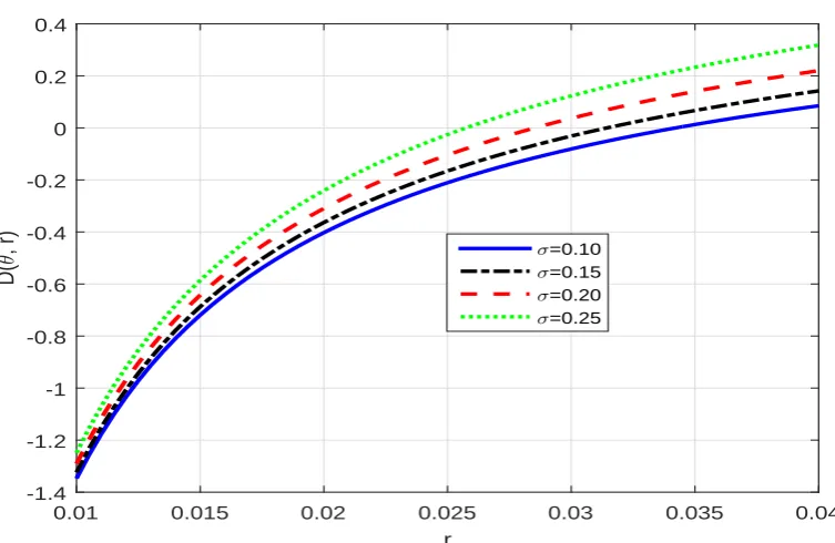
Figure 3 illustrates howr∗varies with labor income uncertainty,σ, for fixed information-processing
cost,λ– the aggregate saving function is increasing with the interest rate and the general
equilib-rium interest rate is decreasing with labor income uncertainty. We can see from Table 4 that if the
economy becomes more volatile (i.e., largerσ), the Kalman gain (θ)increases while the
equilib-rium interest rate(r∗)decreases. This result is different from that obtained in the fixed capacity
case in whichθ and r∗ move in the same direction. (See Table 2.) The main reason for this
re-sult is that income uncertainty affects the equilibrium interest rate via two channels: (i) The direct
channel which leads to higher aggregate savings (i.e., the ω2
ζ term in (38)) and (ii) the indirect
channel which leads to lower aggregate savings (i.e., the θr∗,eλ term in (38)), and the direct
channel dominates.28 In the next section, after estimating the income process using the U.S. data,
we will examine how changes in income uncertainty affects the level of optimal attention and the equilibrium interest rate, and the relative volatility of consumption and wealth to income.
It is worth noting that the analysis in the benchmark model can be extended to an economy with risky financial assets, which consumers can use to partially hedge their idiosyncratic labor
income shocks. Under some reasonable assumptions, the general equilibrium results obtained in our benchmark model remain valid when we reinterpret the variance of the labor income as the
variance of the residual risk faced by the consumers after hedging using the risky financial assets.29
4. Empirical and Quantitative Results
In this section we assess our GE-RI model’s implications for the dynamics of consumption, income
and wealth. To construct empirical counterparts that are comparable with the theoretical moments derived in the model, we construct a panel with individual consumption, income and wealth based
on the Panel Study of Income Dynamics (PSID) and the Consumer Expenditure Survey (CEX), us-ing the imputation approach from Blundell, Pistaferri, and Preston (2008) as extended by Guvenen
and Smith (2014). Then, using the estimated income process, we show the GE-RI model signifi-cantly fits the data better than the full information model in terms of the consumption and wealth dynamics. Our closed-form solutions explicitly show the different channels through which RI
drives the results.
4.1. Empirical Evidence
In order to measure the relative consumption dispersion in the data, sd(∆c)/ sd(∆y), we
con-struct a panel data set which contains both consumption and income at the household level. The
PSID does not include enough consumption expenditure data to create full picture of household nondurable consumption. Such detailed expenditures are found, though, in the CEX from the
Bureau of Labor Statistics. But households in this study are only interviewed for four consecu-tive quarters and thus do not form a panel. To create a panel of consumption to match the PSID
income measures, we use an estimated demand function for imputing nondurable consumption following Guvenen and Smith (2014). Using an IV regression, they estimate a demand function for nondurable consumption that fits the detailed data in the CEX. The demand function uses
demo-graphic information and food consumption which can be found in both the CEX and PSID. Thus, we use this demand function of food consumption and demographic information (including age,
family size, inflation measures, race, and education) to estimate nondurable consumption for PSID households, creating a consumption panel.
Following Blundell, Pistaferri, and Preston (2008), we define the household income as total household income (including wage, financial, and transfer income of head, wife, and all others
in household) minus financial income (defined as the sum of annual dividend income, interest income, rental income, trust fund income, and income from royalties for the head of the household
only) minus the tax liability of non-financial income. This tax liability is defined as the total federal tax liability multiplied by the non-financial share of total income. Tax liabilities after 1992 are
not reported in the PSID and so we estimate them using the TAXSIM program from the National Bureau of Economic Research. Our final household income measure can be expressed as:
income measure=(total HH income−financial income)−taxes×total HH income−financial income
total HH income .
Our household sample selection closely follows that of Blundell, Pistaferri, and Preston (2008)
as well.30 We exclude households in the PSID poverty and Latino subsamples. We exclude
house-holds in years of family composition change, change in marital status, or female headship, as well as in years where the head or wife is under 30 or over 65. Households in years with missing
ed-ucation, region, income, and imputed consumption responses are also excluded. We also exclude households in years where they report a negative income or a food consumption level in the top or
bottom 5 percent of all reported values in that year. Income and consumption values are then
de-flated by the CPI to constant 1982−1984 dollars. Our final panel contains 7, 111 unique households
with 58, 034 yearly income responses and 48, 990 imputed nondurable consumption values.31
With this constructed panel of household income and consumption, we next drop households
in years where year-over-year food consumption changes are more than 20 percent or less than−20
percent. To exclude extreme outliers, we then follow Floden and Linde (2001) and normalize both income and consumption measures as ratios of the mean of each year, and exclude household in
bottom and top 1 percent of the distribution of those ratios. Figure 4 shows the relative dispersion of consumption, defined as the ratio of the standard deviation of the consumption change to the
standard deviation of the income change between 1980 and 2000. The basic pattern confirms but extends the findings in Blundell, Pistaferri, and Preston (2008) – relative consumption dispersion
declines in the 1980s, but this decline stops around 1990.
In order to calculate the relative volatility of wealth to income ratio,sd(∆a)/ sd(∆y), we use
wealth information included in the PSID data. Notice that the PSID only reports household wealth
variables every five years starting in 1983, and then every other year starting in 1998. To be con-sistent with the model, we construct household wealth in the following way. We use measure of
wealth defined as the sum of the net value of liquid assets (checking, savings, money market, etc.), vehicles, home equity, and other assets such as bonds, insurance policies, and trusts. All reported
30They create a new panel series of consumption that combines information from PSID and CEX, focusing on the
pe-riod when some of the largest changes in income inequality occurred. For other explanations for observed consumption and income inequality, see Krueger and Perri (2006) and Attanasio and Pavoni (2011).
31There are more household incomes than imputed consumption values because food consumption - the main input
values are again deflated by the CPI to constant 1982−1984 dollars. We normalize each reported wealth and income value to the mean of the year reported, and then exclude outliers of this dis-tribution at the top and bottom 1 percent. We then take the standard deviations of the change in
normalized value from the previous report for both wealth and income to calculate our ratio. Our final panel for wealth and income has 23, 630 observations across 6232 households. This panel is
somewhat smaller than our panel of consumption and income due to the limited number of years that wealth measures are reported. Figure 5 reports the results, which shows the relative volatility
of wealth to income has been relatively stable in the sample period.
When estimating the income process, we focus on the sample period to the years 1980−1996,
due to the PSID survey changing to a biennial schedule after 1996. To further restrict the sample to exclude households with dramatic year-over-year income changes, we eliminate household in-comes with year-over-year level changes in the top and bottom 5 percent of the distribution in each
year. Then, again following Floden and Linde (2001), we normalize household income measures as ratios of the mean for that year and exclude all household values in years in which the income is in
the top and bottom 1 percent of the normalized income measure for the year. To eliminate possible heteroskedasticity in the income measures, we follow Floden and Linde (2001) and regress each on
a series of demographic variables in a fixed-effect panel regression to remove variation caused by differences in age and education. We next subtract these fitted values from each measure to create
a panel of income residuals. We then use this panel to estimate the household income process as specified by equation (4) by running panel regressions on lagged income. As the last row of Table
1 reports, the estimated values ofφ0,φ1, andσare 0.0005, 0.919, and 0.175, respectively.
4.2. Empirical Implications for the Cross-Sectional Dispersion of Consumption, Wealth, and
Income
Luo (2008) examines how RI affects consumption volatility in a partial equilibrium version of the PIH model presented above. In general equilibrium, since RI affects the equilibrium interest rate,
it will have an additional effect on consumption dynamics. Using (29) and (30), we can obtain the key stochastic properties of the joint cross-sectional dispersion of individual consumption and
wealth relative to income. The following proposition summarizes the implications of RI for the relative dispersion of consumption to income as well as the relative dispersion of financial wealth
to income. Note that mathematically, the cross-sectional dispersion of consumption and wealth (relative to income) can be measured by the relative volatility of consumption to income and the
Proposition 4. Under RI, the relative volatility of individual consumption growth to income growth is
µcy≡ sd( ∆c∗t)
sd(∆yt) =
r∗
1+r∗−φ1
r
(1+φ1)Γ(θ,r∗)
2 , (39)
and the relative volatility of financial wealth to income is
µay ≡ sd( ∆a∗
t)
sd(∆yt) =
1 √
2(1+r∗−φ1)
s
1−φ1+ r
∗2(1−θ) (1+φ 1)
1−(1−θ) (1+r∗)2+
2r∗(1−θ) 1−φ2
1
1−φ1(1−θ) (1+r∗).
(40)
Proof. See Appendix 7.1.
Expression (39) shows that RI has two opposing effects on the relative consumption
disper-sion. The first effect is direct through its presence in the expression ofΓ(θ,r∗), whereas the second
effect is through the general equilibrium interest rate(r∗)and is thus indirect. Using the
expres-sion ofΓ(θ,r∗), it is straightforward to show that the direct effect of RI is to increase consumption
volatility. The intuition is very simple: the presence of the RI-induced noise dominates the slow adjustment of consumption in determining consumption volatility at the individual level. In
con-trast, the indirect effect of RI will reduce consumption volatility because it reduces the general
equilibrium interest rate and∂Γ(θ,r∗)/∂r∗ > 0. Following the literature of precautionary savings
and the estimated income process in the preceding subsection, we setρ = 0.04,α= 3,σ =0.175,
andφ1 =0.919. The second to fourth rows of Table 2 reports how the interest rate and the relative
volatility of consumption and wealth to income vary withθin general equilibrium whenψ=0.54.
It is clear from the second row of Table 2 that RI can significantly affect the equilibrium interest
rate. For example, whenθdecreases from 1 to 0.10,r∗decreases from 3.41 percent to 2.89 percent,
which is very close to 2.97 percent, the average annual equilibrium real interest rate from 1980 to
1996 estimated in Laubach and Williams (2015) using 1961−2014 U.S. quarterly data (note that if
θ = 0.11, the equilibrium interest rate obtained in our model is exactly the same as its empirical
counterpart). Here we focus on the 1980−1996 period because we use it to estimate the income
process and the relative volatility of consumption to income.
From the third row of Table 2, the relative volatility of consumption growth to income growth
increases with the degree of inattention. For example, whenθdecreases from 1 to 0.1,µcyincreases
from 0.290 to 0.375, which is the same as the empirical counterpart. It is clear from these results that
the direct effect of inattention via theΓ(θ,r∗)term in (39) dominates its indirect general
equilib-rium effect viar∗. We can get the same conclusion by shutting down the general equilibrium (GE)
Com-paring the GE and PE results in Table 2, we can see the values ofµcyare lower in the GE case if the
interest rate is fixed asθ decreases. In other words, the general equilibrium effect of RI tends to
reduce the volatility of individual consumption in this case.32 Furthermore, from the second panel
of Table 2, we can see that the equilibrium relative volatility of consumption to income increases with the EIS. The main reason for the result is that the equilibrium interest rate increases with the
EIS. Note that the higher the value of the EIS, the higher the dissaving effect due to impatience, and the higher the equilibrium interest rate.
Another important implication of RI in general equilibrium is that RI leads to more skewed
wealth dispersion measured byµay, the relative volatility of financial wealth to labor income. From
the fourth row of Table 2, we can see that whenθis reduced from from 1 to 0.1,µayincreases from
1. 748 to 2.62 in theψ=0.54 case, which is much closer to the empirical counterpart. (For example,
µay is 3.11 in 1993 and is 2.59 in 1998.) From (30), it is clear that the main driving force behind
this result is the presence of the estimation error, st−bst, because ∂var(st−bst)/∂θ < 0. Note
that although∂r∗/∂θ>0, the estimation error channel dominates the general equilibrium channel
and increases wealth dispersion. Therefore, RI also increases wealth inequality, which makes the
model fit the data better.33 We can also see from the second panel of Table 2, the equilibrium
relative volatility of wealth to income increases with the EIS. The main reason for the result is that the equilibrium interest rate increases with the EIS. We can clearly inspect this mechanism by
considering a special case whenφ1 =1. Specifically, in this case, (30) reduces to
µay=
s
1−θ
1−(1−θ) (1+r∗)2, (41)
which implies thatµayincreases withψandr∗.
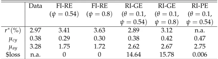
To briefly summarize the key discussions above, Table 3 compares the performances of the
FI-RE model, the general equilibrium rational inattention model (RI-GE), and the partial equilibrium rational inattention model (RI-PE) with the data. Overall, it shows under the estimated income
process and at a single value of rational inattention parameter (θ), the GE-RI model can do a
sig-nificantly better job than the FI-RE model in generating a lower interest rate, a higher consumption
volatility, and a higher wealth volatility, bring all of them much closer to the data. In terms of wel-fare loss, as the last row in Table 3 shows and will be discussed in detail in the next subsection, the
32We cannot examine the stochastic properties of aggregate consumption dynamics because all idiosyncratic shocks
(income shocks and RI-induced noise shocks) cancel out after aggregating across consumers.
33The literature has found that simple models based on standard CRRA preferences and on measured uninsurable
partial equilibrium model significantly underestimates the welfare loss, though the welfare loss is generally small.
Table 4 reports how elastic Kalman gain, the general equilibrium interest rate, and the relative
volatility of consumption and wealth to income vary with different values of income uncertainty
measured byσ(andσy). We have reached four key findings. First, it is clear from the second row of
Table 4 that the Kalman gain increases with income volatility. For example, ifλ = 0.38 (the value
calibrated to the data as explained in the next paragraph) andψ=0.54,θincreases from 0.11 to 0.15
whenσincreases from 0.2 to 0.4. This means agents optimally allocate more attention to the state
variable when income uncertainty increases. Second, RI has significant effects on the equilibrium
interest rate. For example,r∗ declines from 2.79 percent to 1.94 percent whenσincreases from 0.2
to 0.4. It is worth noting that in the elastic capacity case an increase in income volatility affects the
equilibrium interest rate via two channels: (i) the direct channel (theω2
ζ term in (38)) and (ii) the
indirect channel (the elastic capacityθ term in (38)). The third panel of Table 4 reports the results
when we shut down the indirect channel and assume thatθ = 1. Comparing the first and third
panels of Table 4, we can see that the indirect channel is more important whenσis relatively low.
For example, given thatσ = 0.2,r∗ decreases from 3.23 percent to 2.79 percent when we switch
from the FI economy to the RI economy, whereasr∗only decreases from 2.14 percent to 1.94 percent
whenσ = 0.4. Third, EIS can significantly affect the dispersions of consumption and wealth via
affecting the optimal attention level and the equilibrium interest rate. For example, whenσ= 0.2
andψincreases from 0.54 to 0.8, the optimal attention level is reduced from 11% to 8% and the
equilibrium interest rate is reduced from 2.79 percent to 2.73 percent. Note that under RI, EIS affects the equilibrium interest rate via two channels: (i) the optimal attention channel and (ii) the impatience-induced dissaving channel. In this quantitative analysis, we can see that the optimal
attention channel dominates the impatience-induced dissaving channel. Consequently, µcy and
µay increases from 0.34 to 0.43 and from 2.53 to 2.87, respectively. Fourth, the relative volatility
of consumption growth to income growth decreases with the value of σ in general equilibrium.
That is, consumption becomes smoother when income becomes more volatile. For example, in the
equilibrium RI economy whenψ=0.54,µcydecreases from 0.34 to 0.21 whenσincreases from 0.2
to 0.4.34
The last finding highlighted above might provide a potential explanation for the empirical evidence documented in Blundell, Pistaferri, and Preston (2008) that income and consumption
34It is not surprising thatµ
inequality diverged over the sampling period they study.35 To explore this issue in our model,
we do the following exercise. First, we divide the full sample into two sub-samples (1980−1986
and 1987−1996) and apply the same estimation procedure to re-estimate σ andφ1 (see the first
and second rows of Table 1 for the estimation results). Household income is more volatile in late
sub-periods than earlier ones. Specifically, the standard deviation ofyis 0.386 in the sub-sample