Annex I and non Annex I countries’productive performance revisited using a generalized directional distance function under a metafrontier framework: Is there any convergence divergence pattern for technology gaps?

Munich Personal RePEc Archive

Annex I and non-Annex I

countries’productive performance

revisited using a generalized directional

distance function under a metafrontier

framework: Is there any

convergence-divergence pattern for

technology gaps?

Kounetas, Kostas and Zervopoulos, Panagiotis

University of Patras, Department of Economics, Greece, Department

of Management, College of Business Administration, University of

Sharjah, Sharjah 27272, United Arab Emirates

15 July 2017

1

Annex I and non-Annex I countries’productive performance revisited using a

generalized directional distance function under a metafrontier framework: Is there any convergence-divergence pattern for technology gaps?

Konstantinos Kounetas a,* and Panagiotis D. Zervopoulos b

a

Department of Economics, University of Patras, Rio 26504, Patras, Greece

b

Department of Management, College of Business Administration, University of Sharjah, Sharjah 27272, United Arab Emirates

Abstract

Countries rapid economic growth, energy consumption and anthropogenic emissions (GHGs) in the atmosphere are creating serious environmental problem on both global and local scales -. This is while compiled evidence about the relationship between climate change/global warming and the amount of GHG released is present (IEA, 2010). In advance, it is generally accepted that countries production processes, should seriously, take into account environmental sustainability principles and targets. In recent years, there have been a series of studies using a directional distance function dealing with environmental efficiency with the aim of measuring the ability of decision making units (i.e regions, firms, industries, countries) to produce more with less impact on the environment. A scarcity of empirical studies appears concerning the estimation of directional distance function under a metafrontier framework. In this paper we employ a balanced panel of 103 countries from 1995-2011 to shed light on the idiosyncratic performance of countries participating in two distinct different groups (Annex I and non-Annex I) using a generalized directional distance function independent of the direction vector length -. The non-parametric metafrontier framework - used in this study, as a first stage of analysis, is exploited to account for the heterogeneity between countries participating in our sample. In the second stage, a convergence-divergence hypothesis has been examined for the technology gaps estimated for each period. Our findings reveal significant patterns between countries’ individual performance.

Key words: Metafrontier; Generalized Distance Function; Technology gaps; Annex-I

countries

*Corresponding Author Department of Economics University of Patras Rio Campus, 26504 Greece

2

1. Introduction

The Intergovernmental Panel on Climate Change (2007) has assessed that over the

last 50 years, global warming has been caused due to anthropogenic greenhouse gas

emissions (GHGs). The impact of GHGs on climate change has been the top agenda

and considered the leading issue for many governments, organizations, economists,

researchers and scholars since it threatens countries’ sustainable development (Tol,

2009; Weitzman, 2009). The significance of this problem is apparent from cases such

as the signing of the Kyoto Agreement in 1997 and subsequent efforts in Copenhagen

and Cancun (2010), Durban and Doha (2011), Warsaw (2013) and latest in Paris

(2015) to reach an international agreement aimed at reducing greenhouse gas

emissions. In the face of climate change repercussions, many countries have devoted a

large portion of their resources towards designing and implementing mitigation to

achieve a satisfactory level of sustainable development while others (headed by U.S)

criticizes insisting on a more voluntary orientation. Furthermore, it is true that Kyoto

climate policies put more attention and emphasis on the reduction of global emissions

to mitigate climate change (Yu-Ying et al., 2013).

The Kyoto protocol was negotiated in 1997 during the Third Conference of the

Parties to the United Nations framework Convention of Climate Change. During its

establishment put into discussion the reduction levels of GHGs, most notably CO2

from fossil fuel combustion, for Annex I and non-Annex I countries in an

international agreement framework (Den Elzen and Höhne, 2008). Moreover, in a

world where economies are linked by international trade and capital flows emissions

abatement of Annex I economies may have, possibly, effect on trade, carbon leakage,

3

(Den Elzen and De Moor, 2002). A further caveat, from the stance of economic

theory, considers large economic adjustment costs to Annex I coutries (Böhringer, C.,

Vogt, C. 2003) or consider possible policies (i.w preferential tarrifs reductions) for

their compesantion (Babiker et al. 2000). Furthermore, some studies report the fact

that recent Kyoto modifications, including U.S decision, boil down climate policies as

business as usual questioning its economic and enviromental impacts for the countries

participated in this commitment (Böhringer and Vogt, 2003; 2004).

The level of ambitions for reducing emissions by developed (Annex I) and

developing (non-AnnexI) countries under the Kyoto agreement was one of the most

important aspects in current climate negotiations. Although there have been many

attempts for the non-AnnexI group to ratify the agreement, several political,

institutional and economic barriers appeared to hinder them (Calbick and Gunton,

2014)1. Thus, the clear distinction for countries participating as AnnexI and

non-AnnexI gathers significant opportunity for engineers, economists, scholars and

politicians to examine the negative impact of human activity, in terms of pollution

equivalents, even at a country level through this perspective. This growing interest in

incorporating undesirable outputs in the production function under the different

technological regimes yields, on the one hand, numerous published articles (see

Zhang and Choi, 2014) while, on the other hand, introduces several methods for

asymmetrically handling the two types of outputs (i.e Tone, 2001; Cheng and

Zervopoulos, 2014).

A common characteristic of these studies is that operates under the assumption

of technological isolation (Tsekouras et al., 2016) examining a rather homogeneous

1

4

group (Feroz et al., 2009; Halkos and Tzeremes, 2014). It may also adopt a

metafrontier production function in a “mechanistic” way creating groups according to

specific criteria ignoring their technological status (Kounetas, 2015). The introduction

of the metafrontier production function (Battese et al., 2004) allows technological

heterogeneity to be incorporated in productive efficiency analysis and therefore

relaxing restrictive technological isolation conditions. In the framework of

technological heterogeneity, any positive influence of technological spillovers from

domestic mitigation strategies onto productive performance may be eliminated, if the

production units are locked-in, or if they exhibit path-dependence of the evolution of

their productive performance (Tsekouras et al., 2016).

In this paper we extent a generalized efficiency measure of a directional distance

function (Cheng and Zervopoulos, 2014) in a methodological framework which

allows the co-examination of (i) efficiency differences in terms of productive

performance for countries operating under two distinct technological regimes, (ii) any

inter-linkages and flows between the two heterogeneous technologies and more

specifically spillover effects on non-Annex I countries (iii) the convergence

hypothesis for technology gaps for the examined set of countries. This analytical

framework is applied to 103 countries over the 1995-2011 period revealing interesting

patterns of productive performance which have not been traced by previous seminal

papers on environmental efficiency.

This study unfolds as follows. Section 2 reviews the literature on directional distance

functions in conjunction with the metafrontier analysis. Section 3 presents the

methodology. Section 4 discusses the selection of input and output variables. Section

5

2. Review of the literature

In efficiency and productivity analysis, directional distance functions (hereafter DDF)

have also become popular since most production processes generate undesirable

output(s) as byproduct(s) (i.e. CO2 emissions for firms or mortality rate for health

systems). The main reason for this increased popularity is the ability of DDF to

expand good outputs while reducing bad since the production process of every entity

has not only an economic but also an environmental and social output (Färe and

Grosskopf, 2000; Färe et al., 2005; Zhang et al., 2013). In this context, many

empirical studies have used DDF to investigate the performance of individual DMUs.

Extant studies apply DDF to measure energy efficiency (Zhang et al., 2013; Zhou et

al., 2012), environmental efficiency (Kounetas, 2015; Kumar and Khanna, 2009;

Caramero et al., 2008), sustainability performance (Zhang et al., 2013) and

eco-efficiency (Oggioni et al., 2011; Picazo-Tadeo et al., 2012; Zhang et al., 2008; Färe et

al. 2007; Kuosmanen and Kortelainenn, 2005)2.

Focusing now on the methodological approaches that have been used to

estimate the abovementioned indexes, the literature classifies three groups according

to their framework. The first group contains transformations of conventional DEA

models including hyperbolic distance functions (Färe et al., 1989) radial measures

(Chambers et al., 1996) and non-radial measures. Τhe second one concerns

modifications on the slack-based measures (Tone, 2001) while the third group

contains several modifications on the directional distance function (Chung et al.,

1997).

Many studies have been recorded incorporating DDFs in order to mostly

measure energy and environmental performance of different DMUs. As mentioned

2

6

above, radial nature of DDF stimulates researchers to develop non-radial measures.

For instance, Färe and Grosskopf (2010) and Zhou et al. (2012) extended it in a

non-radial model and Mahlberg and Sahoo (2011) proposed a non-non-radial Luenberger

indicator. Extending the DDF, Zhang et al. (2013), Choi et al. (2012) and Zhou et al.

(2006) developed several slack-based measures for environmental performance while

Fukuyama and Weber (2009) proposed a slacks-based efficiency measure of

efficiency combining the ideas of DDF and SBM. In addition, Zaim and Taskin

(2000) and Cuesta et al. (2009) developed a hyperbolic efficiency measure while

Fukuyama et al. (2011) and Barros et al. (2012) with DDFs proposed slacks-based

measures and weighted Russell DDF. Sueyoshi et al. (2010) presented a

Range-Adjusted measure model for US coal-fired power plants. Finally, Chang and Hu

(2010), Färe and Grosskopf (2010) and Cheng and Zervopoulos (2014) put forth a

generalized non-radial DDF while Zhang et al. (2014) presented a sequential

generalized directional distance function.

On the other hand, very few studies have taken the potential technology

heterogeneity into consideration. First, Oh (2010) using a Malmquist-Luenberg

productivity index incorporated group heterogeneity while Kounetas (2015), Chiu et

al. (2012) and Yu-Ying Lin et al. (2013) measured, not only technology gaps, but also

environmental efficiency technology gaps exploiting the scarcity of similar studies

under the presence of heterogeneity.

3. Methodology

Our methodological framework is developed in two interconnected stages. In the

first stage, we present the theoretical and methodological underpinnings regarding the

estimation of the generalized directional distance function and we discuss the

7

inclusion. In the second stage, we present the theory concerning the convergence

hypothesis using a stochastic kernel approach.

3.1 Definitions, notation and technological gaps

The inputs

1

( ,..., ) m m

x x x  _ are used to produce desirable outputs

1

( ,..., ) s s

y y y  _ and undesirable outputs ( ,...,₁ ) p p

b b b  _ (i.e. CO2 emissions).

In this context, the technology is described as follows:

T x( ) {( , ) : can produce ( , )} y b x y b (1)

where m s p

T  _ _ _, which represents the input - desirable output - undesirable

output bundles that are technologically achievable.

The desirable outputs (y) are jointly produced with the undesirable outputs

(b), modelled as follows:

if ( , )y b T x( ) and b0 then y0 (2)

The assumptions that the technology satisfies are: (a) closedness, (b) free

disposability of inputs and desirable outputs:

( , )x y T, if 'x x and 'y y then ( ', ')x y T

     , (c) weak disposability of

undesirable outputs:  ( , )x b  T ( ,x



b)  T



1, (d) no free lunch:

if ( , , )x y b T and x0 then y0 and b0, (e) doing nothing is feasible:

(0,0,0)T , and (f) convexity (Färe et al., 1994).

The technology is described by the following directional distance function

(DDF):

D x y b g g gT( , , ; x, y, b)sup{ : ( xg yx, g by, gb)T x y b( , , )} (3)

where β denotes inefficiency and the non-zero g(g g gx, y, b) expresses the direction

vector of the inputs, desirable outputs, and undesirable outputs, respectively. The

expression (3) reflects simultaneous reduction in inputs, expansion of desirable

outputs and contraction of undesirable outputs. Drawing on expression (3), the

efficiency is defined as follows: 1 1

 

8

In this study, a generalized directional distance function (GDDF) is applied to

measure environmental efficiency put forth by Cheng and Zervopoulos (2014).

According to this generalized DDF, which is also based on expression (3) and

satisfies the assumptions of the technology set, the efficiency is measured by the ratio:





1

1 1

1

1 /

1

1 / /

m

i io

i

s p

r ro t to

r t

g x m

g y g b

s p



 



 



 









where gi/xio expresses the proportion of

the reduction in inputs, and g_r /y_ro and g_t /b_to indicate the proportion of the expansion and contraction of desirable and undesirable outputs, respectively. The

efficiency measures obtained from this generalized DDF are units invariant,

monotone, translation invariant provided that the Variable Returns to Scale (VRS) technology applies, and reference set invariant (Tone, 2001; Färe and Grosskopf, 2010). Unlike the conventional DDF, the generalized DDF that is used in this study

yields efficiency scores independent of the length of the direction vector (g).

Moreover, like the conventional DDF, this generalized DDF produces efficiency

scores that are consistent with those obtained from radial models.

In the case where multiple technologies (e.g. k distinct technologies, where

1,...,

k K) are present, the input – desirable output – undesirable output sets are

grouped into k technologically feasible sets (i.e. 1 2

, ,..., K

T T T ). The collection of all

input-output feasible combinations of the operational units (e.g. countries) construct

the smallest convex set that is known as metatechnology set, denoted by meta

T

(Battese and Rao, 2002; Battese et al., 2004; O’Donnell et al., 2008). The metatechnology set is modelled as follows:

meta( ) {( , ) : can produce ( , )}

T x  y b x y b (4)

and the group-specific technology set is described as follows:

k( ) {( , ) : used by operational units in group can produce ( , )}

T x  y b x k y b (5)

Hence, meta( ) { ( )1 2( ) ... K} T x  T x T x  T .

By introducing the generalized DDF (Cheng and Zervopoulos, 2014) into the

metatechnology framework, we measure the metaefficiency and group-specific

9





1 1 1 1 1 / ( , , ; , , ) 1

1 / /

meta

m _{meta k}

i io

i

k k k

x y b

T _{s p}

meta k meta k

r ro t to

r t

g x m

D x y b g g g

g y g b

s p           







1 1

. . 1,...,

K n

k k k meta

j ij io x

k j

s t  x x  g i m

    



1 1 1,..., K n

k k k meta

j rj ro y

k j

y y g r s

      



1 1 1,..., K n

k k k meta

j tj to b

k j

b b g b l

      



1 1 1 K n k j k j    



k 0 j

  (6)





1 1 1 1 1 / ( , , ; , , ) 1

1 / /

k

m _{k k}

i io

i

k k k

x y b

T _{s p}

k k k k

r ro t to

r t

g x m

D x y b g g g

g y g b

s p           







1

. . 1,...,

n

k k k k

j ij io x

j

s t v x x  g i m

   



1 1,..., n

k k k k

j rj ro y

j

v y y  g r s

   



1 1,..., n

k k k k

j tj to b

j

v b b  g b l

   



1 1 n k j j v  



k 0, 1,...,

j

v  k  K (7)

where kj and k j

v represent the optimal weights assigned to inputs and outputs. In our

10

Using programs (6) and (7), we can calculate the technology gap ratio (Battese

et al., 2004) or the reciprocal relationship of the metatechnology ratio (MTR) (O’Donnell et al., 2008).









1 1 1 1 1 1 1 1 / 1

1 / /

MTE( , , )

0 MTR( , , ) 1

1

TE( , , ) _{1 /}

1

1 / /

m _{meta k}

i io

i

s _{meta k} p _{meta k}

r ro t to

r t

m _{k k}

i io

i

s _{k k} p _{k k}

r ro t to

r t

g x m

g y g b

x y b s p

x y b

x y b

g x m

g y g b

s p                        













(8)

where MTE expresses the technical efficiency of an operational unit with respect to

the metatechnology, and TE represents the technical efficiency of an operational unit

with respect to the k group frontier.

The metafrontier framework provides benchmarking for all operational units

independently from the group-specific frontier that each unit belongs. As a result,

drawing on the technology heterogeneity concept, we can attribute differences,

captured by technology gaps, due to: (a) the structure of national markets, (b) national

regulations and policies, (c) cultural profiles and legal and institutional frameworks

(Halkos and Tzeremes, 2011), (d) available resource endowments, (e) economic

infrastructure, (f) characteristics of the physical, social and economic environment in which production takes place (O’Donnell et al., 2008; Kounetas et al., 2009), and (g) knowledge characteristics and strategic orientation (Kontolaimou and Tsekouras,

2010). In this context, a value of the MTR closer to unity indicates smaller technology

heterogeneity while a value closer to zero denotes greater technology heterogeneity.

In addition to the identification of technology heterogeneity, the

metatechnology framework facilitates the measurement of technology gaps (TG).

Chiu et al. (2012) defined the TG inefficiency as the distance between the individual

frontier and the metafrontier. The TG is obtained as follows:

TG( , , ) TE (1 MTR( , , ))x y b    x y b (9)

We present a graphical analysis (please see Fig.1) of the world metafrontier and

the two individual frontiers for the output-oriented framework. At a given input and

output level, say x and y the observed country A under the non-Annex I technology

11

frontier) between points A and B, the metatechnical inefficiency between points A

and C (MGDDF relative to the metafrontier) and the technology gap difference

denoting as TG.

3.2 The Technology Gaps’Stochastic Convergence Hypothesis

Thus we can consider technology gap (TG)3 as a continuous-time stochastic

process



X t( ), t0



and assume that the each stochastic process is a

continuous-time Markov chain with distribution function _t. Each satisfies the Markovian

property Prob(X_t A X_j, jt X; x)Prob ( , ) x A , with A E where is

the space state of , i called “stochastic kernel” and under certain conditions

(Quah, 1997) satisfies the following equation _t ( , ) d_t

E

x A x 

_ 



 that leads to

( ) ( ) ( )d

t t

E

f_ y 



f_ y x f x x with f xt( ) and f y x( ), which are respectively the density

function of _t and Prob, if they exist.

The empirical estimate of the marginal probability density function (pdf) of x is

given by: 2 2 ₁ 1 2 2 1

1 1 1

ˆ_{( )} ˆ_{( , )d d}

2 2 j j y x y y x x n h h

j _{x y}

f x f x y y e e y

n h



h



    _{ }                    









2 1 2 1 1 1 2 j x x x n h j _x e

n h



          





(10)

where the joint distribution ( , )f x y is obtained using a product of Gaussian kernel K

(Fotopoulos, 2006): 2 2 ₁ 1 2 2 1

1 1 1

ˆ_{( , )}

2 2 j j y x y y x x n h h

j x y

f x y e e

n h



h



    _{ }             _   



3

12

1

1 1 1

n

j j

j x x y y

x x y y

K K

n _ h h h h

 

 

 

  _{ }

  _{ }

 





(11)

where hx and hy are bandwidths calculated with the direct plug method applied

separately in each dimension. In this way, a nonparametric estimation of the

stochastic kernel4 is given by:

ˆ( ) ˆ( , )_ˆ ( ) f y x f y x

f x

  (12)

The stochastic kernel may be interpreted as a transition matrix with a continuum

of rows and columns. Let a time interval of length  ; the relationship among two

distributions over  can be written as:

f_{t }( )y f y x f x x_( ) ( )d_t 









(13)

Following the approach developed by Johnson (2000 and 2005) and Fotopoulos

(2006), the long-run ergodic distribution is found as the solution to:

f ( )y f y x f_( ) ( )dx x



 







(14)

One possible way to face this problem is through a discretization of the time

interval [ , ] b by partitioning it in n non-overlapping subintervals, then is possible to

estimate ( | ) with midpoints of these subintervals. If ( | )

( ) are defined and is sufficiently large (which leads to ∑ ( | ) )

then the matrix { } has the same structure as a transition probabilities

matrix and { } may be seen as the conditional probability mass function. The

ergodic density can be evaluated as ( ) , where is the rescaled (unit

4

13

sum) left eigenvector corresponding to the unity eigenvalue (also the largest one) of

the matrix .

4. Data Sources and Variable Definitions

To investigate the issues surrounding our main research question we have devised a

unique dataset by employing and matching distinct, but complementary, information

sources. The resulting dataset is a balanced panel consisting of 103 countries for the

1995-2011 period and our final panel dimension comprises of 1751 observations. We

should note that our sample is affected by the events of the global financial crisis that

manifested from August 2007 onwards but also covers the period before and after

Kyoto’s implementation. It is worth adding that the sample period was chosen purely

on the basis of availability of key variables, some of which become unavailable after

1995.

For the estimation of productive efficiency with respect to each country

frontier and the specific metafrontier as well, we employ a multi-input –

single-desirable output- single-unsingle-desirable output data set. More specifically, we

approximate the output variable (Y) by the Gross Value Added of each industry as the

desirable output and CO2 emissions in metric tonnes (Mt) as the undesirable one. For

the input side, we include the capital stock (K) in million Dollars, the labor input (L)

which is captured by the total hours worked by employees, expenditure on

intermediate inputs (M) in million Dollars and the total energy consumption (E)

measured in million tons (Mt) of oil equivalent. Table 1 provides the definition,

measurement and basic descriptive statistics for each variable.

As already mentioned, the data were drawn by combining several distinct sources

14

intermediate inputs were obtained from the World Bank database (World Bank

Developing Indicators), Enerdata-Odyssey database was used to collect data on

energy consumption and CO2. Finally, data on capital were acquired through OECD

Structural Analysis and World Bank databases respectively. The deflators used to

convert the current into constant 2005 prices are specific to each country. At this

point, we should mention that the distinction in two specific frontiers (AnnexI and

non-AnnexI) has been held following the distinction of Kyoto’s protocol.

5. Empirical Results and Discussion

The presentation and discussion of the empirical results follows the two stage

structure of the methodology section.The country specific efficiency scores with

respect to the two groups are firstly presented and discussed.Subsequently, the

metatechnology efficiency scores, the associated metatechnology ratios and

technology gaps which arises in the context of the metafrontier have been used for the

examination of our hypothesis. At the end, the results from the estimation of the

stochastic kernel for the technology gaps has been presented.

5.1 Efficiency,Metatechnology ratios and Technology Gap Estimates

Productive efficiency scores with respect to the specific technology and the

metatechnology, the associated metatechnology ratios and technological gaps are

estimated for the 103 countries in each of the 17 years. GAMS is used to solve the

linear problem of the generalized distance function expanding its use in also the

metatechnology (Cheng and Zervopoulos, 2014). At this point, it is crucial to note that

both the productive efficiency and technology gap estimations are grounded on a

15

individual production set. Therefore, the values of the estimated productive efficiency

and technology gap for each country encompass two dynamic factors. First is the

change of the distance from the (meta-) frontier, while the second is the movement

outwards (technical change) or inwards (technical regress) of the metafrontier itself.

Using this logic, the estimated time-series for efficiency and technology gaps reflect

the diachronic evolution of productive performance of the examined country,

considering any technological developments either in the industry-specific frontier or

in the metatechnology.

Mean values of productive efficiency for each frontier, the metafrontier and

the associated technology gaps are calculated in Table 3. The sample average of

metatechnical efficiency is 0.827. This implies that countries operate at the average

values of outputs and inputs have the potential to increase their GDP and

simultaneously, decrease their CO2 emissions by about 17.3%. Furthermore, it is

quite interesting to mention the slightly difference between AnnexI and non-AnnexI

countries regarding their efficiency performance (0.886 against 0.847) with respect to

their frontier but also the significant difference for their performance with respect to

their metafrontier (0.878 against 0.799). The same holds for technology gaps with the

corresponding values to be 0.029 for the AnnexI and 0.167 for the non-AnnexI.

Furthermore, a Kruskal-Wallis test has been applied to examine the technology

frontier differences between the AnnexI, non-AnnexI countries. The result shows that

the value of this test is 203.17 and thus, the two groups have distinct technology

frontiers with respect to their meta-efficiency productive performance.

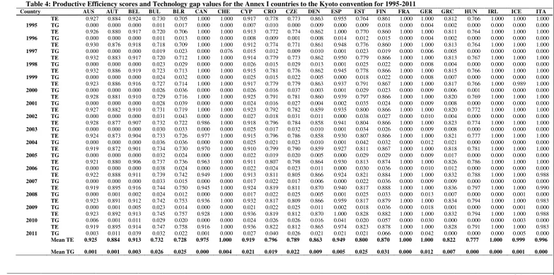
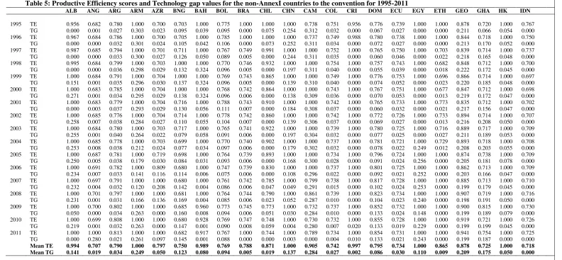
Tables 4 and 5 display the estimated values of (i) the productive efficiency

with respect to the specific technology and (ii) the technology gap with respect to the

16

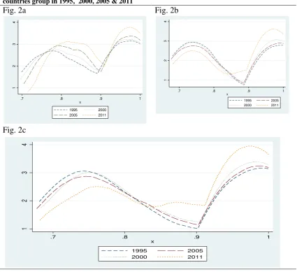
productive efficiency are also given in Fig.2 which shows kernel density estimates for

the first period of the sample (1995), two middle periods (2000 and 2005), and the last

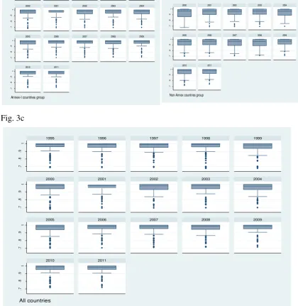
(2011). Furthermore, the time evolution of metatechnology ratios for the two groups

and the total sample are depicted in Fig.3.

We begin by looking at the estimated productive efficiency and technology

gap values for Annex-I countries. From our results it is clear that countries like

Germany, France, the Czech Republic, Ireland, Latvia, the Netherlands, New Zealand,

Slovenia, Sweden Turkey, UK and USA exhibit the highest scores for productive

efficiency constructing the Champions group, while Bulgaria, Belarus, Croatia and

Hungary perform the worst (the laggards group). Furthermore, examining the

efficiency scores with respect to the metatechnology, Canada, France, Ireland, Italy,

Japan, Malta, Norway, Turkey, UK and USA present the smallest technology gaps

and constitute, diachronically, the metafrontier. In contrast, a group of countries like

Lithuania, Latvia, Poland, Portugal, Romania, Slovakia, and Ukraine perform worst

among the remaining ones suggesting that significant knowledge spillover effects are

not in operation within country-specific technologies. Latvia and New Zealand

interestingly, though a champion under the AnnexI frontier, also maintain a large

technology gap, suggesting some strong allocative inefficiencies.

Shifting attention towards to the non-AnnexI technological frontier given in

Table 5, the sample average productive efficiency scores reveal that Armenia, China,

Hong-Kong, Egypt, Mexico, Singapore and South Korea perform identically on

average. However, it is quite interesting that only 4 of 66 (6.02%) of them

diachronically define the metafrontier. Indonesia, Iran, Philippines and Singapore

define the metafrontier more often than any other counterpart whilst Armenia,

17

accompanied from the significant low TGs scores for the specific group support the

idea of significant knowledge incoming spillover barriers from the metatechnology

(Tsekouras et al. 2016). Possible explanations arises from the specific nature of the

agreement for non-Annex I countries (Böhringer and Vogt, 2003; 2004), the role of

appropriability conditions (Castellaci, 2007), the degree of openness to foreign

competition, mainly via globalization, the assymetric effect of technological

opportunities and the size of the market (Los and Verspagen, 2006).

The time evolution of the productive efficiency scores, using the

corresponding kernel densities, for the total sample, depicted in Fig.2c, reflect a

process of continuous and quite significant divergence only for the 2011 period. This

is reflected in the increased deviation of the distribution. The specific result provides

valuable information for the impact of the Kyoto protocol on environmental

performance since 2011 is only one year from its expiration. On the other hand, it is

quite interesting the small but noticeable deterioration in 2005 year during the Kyoto

transition period. The corresponding time evolution of the AnnexI (Fig.2a) reveals

that, although the overall picture is quite similar to the one sketched for the total

sample, a significant increase of the productive efficiency scores were especially

significant during the period. Fig.2b offers the time evolution of the productive

efficiency scores of the non-Annex I group. Notwithstanding this, the distribution

remains almost steady with no apparent divergence or convergence processes in

operation.

Finally, the box-plots of diachronic performance of metatechnology ratios

provide more insight into the distribution among AnnexI, non-AnnexI and the total

sample. In Fig.3c a box plot graph of the estimated metatechnology ratios of the total

18

are diachronically constant with no significant fluctuations. It is clear that Annex-I

countries yield the best average and variance of metatechnology ratios compared with

non-Annex-I and the total sample with a distribution skewed to the right (see Fig.3a).

Moreover, the metatechnology ratios slightly decrease in the 2002-2005 period but

exhibit a drastic increase over the 2005-2011. In contrast, Fig.3b mirrors a rather

different, compared to the AnnexI case, pattern of the non-AnnexI metatechnology

ratios performance. More specifically, it seems that between 1995 and 2001

technology gaps remain quite distant while for the 2002-2008 period a significant

decrease has occurred. On the contrary, in the time window from 2009 to 2011, a

considerable increase emerged. In the same direction, but more impressive, is the

picture of the total sample metatechnology ratios distribution presented in Fig.3c.

5.2 Stochastic Kernel of Annex I and non-Annex I Technology Gaps

The non parametric methodology of stochastic kernel adopted in this study,

refers to the “convergence literature”, typified by the seminal papers by Barro and

Sala-i-Martin (1991) and Mankiw et al. (1992) exploring beta-convergence.However,

according to Quah (1993) stochastic Kernels describes the law of motion of a

sequence of distribution and it serves to retrieve the evolution of the probability

distribution of a random variable (usually GDP) along time allowing it to overcome

the limitations of conventional convergence analysis focus on the dynamic properties

of the series.Stochastic Kernel (Quah, 1996, 1997) resulted in the literature from the

necessity to substitute discrete transition matrices. In this way, stochastic kernels can

be achieved by estimating the density function of a distribution over a given period,

19

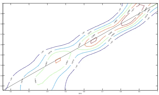
We examine the convergence-divergence hypothesis for technology gaps. The

stochastic kernel in Fig.4 shows how countries’ technological gaps in 1995 evolves

into 2011.Thus, over the 17 years, a three peaks property appears. Each specific peak

reflects a comparatively substantial number of observed transitions from a part of the

distribution to another while having a constant point x-axis. We can understand the

estimated distribution of technology gapsin 2011 at its initial level in 1995. A large

portion of the probability mass is concentrated along the 45o diagonal while the

existence of three peaks along the diagonal indicates the presence of individual

convergence clubs for all the 103 countries. More specifically, there are two local

maxima in both low and high technological gaps parts and a third in the middle part of

relative ones.

Considering the corresponding contour plot in Fig.5, we notice that during the

examined period, countries have a low probability of changing their relative position

in one year in terms of technological gaps suggesting that the mobility is low. The

three peaks phenomenon for technological gaps directly links productivity

differentials and technology structure. This could be further explained in terms of

factor accumulation deformations, factor prices change that acts as an inducement for

the introduction of new technologies (Binswanger et al., 1978) and localized

technological change (Antonelli, 2006; Mulder and DeGroot, 2012). Factor

accumulation distortions (Easterly and Levine, 2001) of the examined countries in

both physical and in terms of human capital could be important to facilitate the

objective of the three clubs creation. For instance, physical capital investment may

embody new energy saving technologies to help in catching up the frontier but this is

20 6. Conclusions

Addressing the problems arising from GHGs emissions released in the environment

and climate change calls for a better understanding of the patterns of CO2 emissions

and country efficiency performance over time. The Kyoto Protocol which imposes

emissions reduction targets on industrialized countires, has been celebrationg as a

milestone in climate protection and mitigation for the world community. In this study,

we apply a generalized efficiency measure of a directional distance function that

allows the directional vector to be independent of the length, under a metafrontier

framework. A particular, however, emphasis is on the construction of a best practice

metafrontier production function that allows for the comparison of two individual

frontiers (AnnexI and non-AnnexIcountries) with completely different technological

regimes.

It has been found that, on average, countries of AnnexI group achieved highest

values of productive efficiency and meta-efficiency performance compared with

non-AnnexI group frontier. Among the countries, Canada, France, Ireland, Italy, Japan,

Malta, Norway, Turkey, UK and USA seem to perform best in their frontier and

metafrontier. In addition, only four countries, Indonesia, Iran, Philippines and

Singapore, report the same for the non-AnnexI countries case.

Moreover, the results with respect to technological gaps report a rather

enlarged differentiation for the two groups. The specific differentiation seems to

acquire a timeless character with completely different behaviors in the two clusters.

The significantly different behavior of the two clusters, in terms of technological

gaps, could strongly depend on differences in local capabilities and on consequential

21

function. Causes of the different behavior of the two frontiers would benefit from

further investigation.

The information yielded investigating the convergence hypothesis with respect

to technological gaps reveals the significant role of spillovers and its inner-flows not

only for each country but also for the two groups. Furthermore, it is related with

general factors as different national policies, level of technology, the ambiguity of the

role of internationalization and lax regulation.

Finally, it should be notes that the results of our study are dependent on the

countires included and the variables used. Further research may be carried out to

extent this study by covering a greater number of countries with a larger period of

examination. Moreover, it is interesting to examine the possible drivers responsible

for the different groups behavior with respect to their productive performance and

22 Acknowledments

The authors are grateful to the participants of the Workshop on the

Econometrics and Statistics of Efficiency Analysis: Recent Developments and

Perspectives, held in "Dipartimento di Scienze dell'Economia" of University of

Salento (Lecce, Italy) on 20-21 June 2015, for their useful comments and suggestions

on earlier versions of this paper and to Kostas Tsekouras for his insightful comments

on earlier versions of this manuscript as well. The author would like to express their

23 References

Antonelli, C., 2006.Localized technological change and factor markets: Constraints

and inducements to innovation. Structural Change and Economic Dynamics,

17(2), 224-247.

Babiker, A., Reilly, M.J., Jacoby, D,H., 2000. The Kyoto Protocol and developing

countries. Energy Policy, 28, 525-536.

Barros, C.P., Managi, S. R. Matousek, R., 2012,. The technical efficiency of the

Japanese banks: non-radial directional performance measurement with undesirable

outputs. Omega, 40, 1–8

Barro, R.J.,Sala-i-Martin, X.,1991.Convergence Across States and Regions. Brooking

Papers on Economic Activity, 1990 (1), 107-182.

Battese, G. E., & Rao, D. P. 2002. Technology gap, efficiency, and a stochastic

metafrontier function. International Journal of Business and Economics, 1(2),

87-93.

Battese, G. E., Rao, D. P., & O'Donnell, C. J. 2004. A metafrontier production

function for estimation of technical efficiencies and technology gaps for firms

operating under different technologies. Journal of Productivity Analysis, 21(1), 91

103.

Binswanger, H.P., Ruttan, V.W., Ben-Zion, U., Janvry, A. D., Evenson, R.E., 1978.

Induced innovation; technology, institutions, and development.

Böhringer, C., Vogt, C. 2003. Economic and environmental impacts of the Kyoto Protocol. Canadian Journal of Economics/Revue canadienne d'économique, 36(2),

475-496.

Böhringer, C., Vogt, C. (2004). The dismantling of a breakthrough: the Kyoto Protocol as symbolic policy. European Journal of Political Economy, 20(3),

597-617.

Calbick, K.S., Gunton, T., 2014. Differences among OECD countries’ GHG

emissions: Causes and policy implications. Energy Policy, 67, 895–902.

24

Camarero, M., Castillo, J., Picazo-Tadeo, A.J., and Tamarit, C., 2013. Is ecofficiency

in greenhouse gas emissions converging among European Union countries.

Empirical Economics , 47(1), 143-168.

Castellacci, F., 2007. Technological regimes and sectoral differences in productivity

growth. Industrial and Corporate Change, 16(6), 1105-1145.

Cheng, G., Zervopoulos, P., 2014. Estimating the technical efficiency of health care

systems: A cross-country comparison using the directional distance function.

European Journal of Operational Research, 238 (3), 899-910.

Chambers, F.G., Chung, Y., Fare, R., 1996. Benefit and distance functions. Journal

of Economic Theory, 70, 407–419

Chiu, C.R., Liou, J.L., Wu, P.I., Fang, C.L. 2012. Decomposition of the

environmental inefficiency of the meta-frontier with undesirable output. Energy

Economics 34, 1392-1399.

Cuesta, R. A., Lovell, C. K., & Zofío, J. L. (2009). Environmental efficiency measurement with translog distance functions: A parametric approach. Ecological

Economics, 68(8), 2232-2242.

Den Elzen, M., Höhne, N. 2008. Reductions of greenhouse gas emissions in Annex I

and non-Annex I countries for meeting concentration stabilisation targets. Climatic

Change, 91(3), 249-274.

Den Elzen, M. G., De Moor, A. P. 2002. Analyzing the Kyoto Protocol under the

Marrakesh Accords: economic efficiency and environmental effectiveness.

Ecological Economics, 43(2), 141-158.

Easterly, W., Levine R., 2001. What have we learned from a decade of empirical

research on growth? It's Not Factor Accumulation: Stylized Facts and Growth

Models. World Bank Economic Review, 15 (2), 177-219.

Färe, R, S. Grosskopf, C. Pasurka 2007. Environmental production functions and

environmental directional distance functions. Energy 32 ,1055-1066.

Färe, R.,and S. Grosskopf 2010. Directional distance functions and slacks-based

measures of efficiency. European Journal of Operational Research, 200 320-322.

Färe, R., Grosskopf, S., Dong-Woon N., Weber, W., 2005. Characteristics of a

polluting technology:theory and practice. Journal of Econometrics, 126, 469-492.

Färe, R., and Grosskopf, S, 2000, Theory and Application of Directional Distance

25

Färe, R., Grosskopf, S., Lovell, C. (1994). Production frontiers. Cambridge University Press: Cambridge.

Feroz, E. H., Raab, R. L., Ulleberg, G. T., & Alsharif, K. 2009. Global warming and

environmental production efficiency ranking of the Kyoto Protocol nations.

Journal of environmental management, 90(2), 1178-1183.

Fotopoulos, G., 2006. Νonparametric Analysis of Regional Income Dynamics: the case of Greece. Economic Letters, 91, 450-457.

Fukuyama, H., Weber, W.L., 2009.A directional slacks-based measure of technical

efficiency. Socio-Economic Planning Science, 43, 274–287

Fukuyama,H., Yoshida, Y., Managi, S., 2011. Modal choice between air and rail: a

social efficiency benchmarking analysis that considers CO2 emissions.

Environment and Economic Policy Studies,13,89-102.

IEA (2010). Carbon Dioxide Emissions from Fuel Combustion. Highlights.

International Energy Agency. OCDE.

Johnson, A.P., 2000. A nonparametric analysis of income convergence across the US

states. Econ. Lett. 69, 219-223.

Johnson, A.P., 2005. A continuous state space approach to "Convergence by Parts.

Economic Letters, 86 (3), 317-321.

Halkos, G. E., Tzeremes, G.N., 2014. Measuring the effect of Kyoto protocol agreement on countries’ environmental efficiency in CO2 emissions: an application of conditional full frontiers. Journal of Productivity Analysis 41 (3),

367-382.

Halkos, G. E., Tzeremes, G.N., 2011 Modelling the effect of national culture on

multinational banks performance: a conditional robust nonparametric frontier

analysis. Economic Modeling , 28, 515–525

IPCC Climate Change 2007. In: Pachauri, R.K., Reisinger, A. (Eds.), Synthesis

Report. Contribution of Working Groups I, II and III to the Fourth Assessment

Report of the Intergovernmental Panel on Climate Change. Core Writing Team.

IPCC, Geneva, Switzerland.

Kontolaimou, A., Kounetas, K., Mourtos, I., & Tsekouras, K. 2012. Technology gaps

in European banking: Put the blame on inputs or outputs? Economic Modelling,

26

Kounetas, K. 2015. Heterogeneous technologies, strategic groups and environmental

efficiency technology gaps for European countries. Energy Policy, 83, 277-287.

Kumar, S., Khanna, N., 2009. Measurement of environmental efficiency and

productivity: a cross-country analysis. Environment and Development

Economics, 14 (4),473–495.

Kuosmanen, T and Kortelainen, M., 2005. Measuring Eco-efficiency of Production

with Data Envelopment Analysis. Journal of Industrial Ecology, 9 (4) 59-72.

Los, B., Verspagen, B., 2006. The evolution of productivity gaps and specialization

patterns. Metroeconomica, 57(4), 464-493

Mahlberg, B. Sahoo, B. K., Luptacik, M., 2011. Alternative measures of

environmental technology structure in DEA: An application. European Journal of

Operational Research, 215(3), 750-762.

Mankiw, N.G., D. Romer, D., D.N. Weil, D.N., 1992. A contribution to the empirics

of economic growth. Quarterly Journal of Economics, 107 (2), 407–437.

Mulder, P., De Groot, L.F.H., 2012.Structural change and convergence of energy

intensity across OECD countries, 1970-2005. Energ. Econ. 34, 1910-1921.

O’Donnell, C. J., Rao, D. P., & Battese, G. E. 2008. Metafrontier frameworks for the study of firm-level efficiencies and technology ratios. Empirical Economics, 34(2),

231-255.

Oggioni, G., Riccardi, R., & Toninelli, R. (2011). Eco-efficiency of the world cement

industry: a data envelopment analysis. Energy Policy, 39(5), 2842-2854.

Oh, Dong-hyun 2010. A metafrontier approach for measuring an environmentally

sensitive productivity growth index. Energy Economics 32 (1), 146-157.

Quah, D.T., 1997. Empirics for Growth and Distribution: Stratification, Polarization,

and Convergence Clubs. Journal of Economic Growth, 2, 27-59.

Quah, D.T., 1993. Galton's Fallacy and the Convergence Hypothesis. Scandinavian

Journal of Economics, 95, 427-443.

Quah, D.T., 1996. Convergence empirics across economies with (some) capital

mobility. Journal of Economic Growth, 1, 95-124.Sueyoshi, T., Goto, M. 2010.

Should the US clean air act include CO 2 emission control?: Examination by data

envelopment analysis. Energy Policy, 38(10), 5902-5911.

Tol R., 2009. The economic effects of climate change. Journal of Economic

27

Tone, K. 2001. A slacks-based measure of efficiency in data envelopment analysis.

European Journal of Operational Research 130, 498-509.

Tsekouras, K., Chatzistamoulou, N., Kounetas, K., Broadstock, D. C. 2016.

Spillovers, path dependence and the productive performance of European

transportation sectors in the presence of technology heterogeneity. Technological

Forecasting and Social Change, 102, 261-274.

Yu-Ying Lin, E., Chen Ping-Yu., Chen, Chi-Chung 2013.Measuring the

environmental efficiency of countries: A directional distance function metafrontier

approach. Journal of Environmental Management 119, 134-142.

Weitzman, M.L., (2009) On modeling and interpreting the economics of catastrophic

climate change. The Review of Economics and Statistics, 91 (1) 1-19

Taskin, F., & Zaim, O. (2001). The role of international trade on environmental

efficiency: a DEA approach. Economic Modelling, 18(1), 1-17.

Zhou,P., B.W. Ang, H. Wang 2012. Energy and CO2 emission performance in

electricity generation: a non-radial directional distance function approach.

European Journal of Operational Research, 221, 625–635

Zhang, N., P. Zhou, Choi Yongrok 2013. Energy efficiency, CO2 emission

performance and technology gaps in fossil fuel electricity generation in Korea: a

meta-frontier non-radial directional distance function analysis. Energy Policy, 56,

28 APPENDIX A

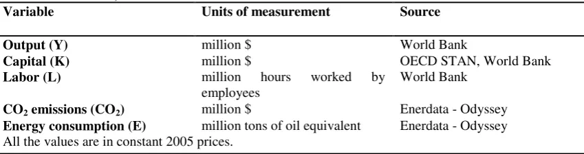
Table 1: Variables, units of measurement and sources

Variable Units of measurement Source

Output (Y) million $ World Bank

Capital (K) million $ OECD STAN, World Bank

Labor (L) million hours worked by employees

World Bank

CO2 emissions (CO2) million $ Enerdata - Odyssey

[image:29.595.88.513.107.219.2]

Energy consumption (E) million tons of oil equivalent Enerdata - Odyssey All the values are in constant 2005 prices.

Table 2: Descriptive statistics by type of agreement and variable

TOTAL Annex-I Non-Annex-I

Y 203,81

(143,1)

125,16 (185,41)

14,64 (18,87)

K 1575,85

(4561,07)

745,14 (658.1)

55,48 (98,49)

L 24.05

(84.06)

12.83 (24.17)

3.91 (4.97)

CO2 231,441

(731,35)

168,15 (125,17)

89,25 (63,25)

E 93,125

(281,76)

65,47 (58,62)

22,01 (17,32)

[image:29.595.88.427.454.560.2]

Note 1: Numbers indicate the mean value while parentheses correspond to the standard deviation

Table 3: Average descriptive statistics for technical, metatechnical efficiency and technology gaps for the individual groups

Technical Efficiency

Meta-technical Efficiency

Technology Gap

Annex-I 0.886

(0.102)

0.878 (0.107)

0.029 (0.011) Non-Annex-I I 0.849

(0.125)

0.799 (0.122)

0.167 (0.103)

ALL 0.869

(0.118)

0.827 (0.122)

[image:30.842.36.819.91.480.2]

29

Table 4: Productive Efficiency scores and Technology gap values for the Annex I countries to the Kyoto convention for 1995-2011

Country AUS AUT BEL BUL BLR CAN CHE CYP CRO CZE DEN ESP EST FIN FRA GER GRC HUN IRL ICE ITA 1995

TE 0.927 0.884 0.924 0.730 0.705 1.000 1.000 0.917 0.778 0.773 0.863 0.955 0.764 0.861 1.000 1.000 0.812 0.766 1.000 1.000 1.000

TG 0.000 0.000 0.000 0.011 0.017 0.000 0.000 0.007 0.010 0.000 0.009 0.000 0.009 0.018 0.000 0.004 0.002 0.000 0.000 0.000 0.000

1996

TE 0.926 0.880 0.917 0.720 0.706 1.000 1.000 0.913 0.772 0.774 0.862 1.000 0.770 0.860 1.000 1.000 0.811 0.764 1.000 1.000 1.000

TG 0.000 0.000 0.000 0.011 0.013 0.000 0.000 0.008 0.009 0.001 0.008 0.014 0.012 0.015 0.000 0.004 0.002 0.000 0.000 0.000 0.000

1997

TE 0.930 0.876 0.918 0.718 0.709 1.000 1.000 0.912 0.774 0.771 0.861 0.948 0.776 0.860 1.000 1.000 0.813 0.764 1.000 1.000 1.000

TG 0.000 0.000 0.000 0.019 0.023 0.000 0.076 0.015 0.012 0.009 0.010 0.001 0.023 0.019 0.000 0.006 0.005 0.000 0.000 0.000 0.000

1998

TE 0.932 0.883 0.917 0.720 0.712 1.000 1.000 0.914 0.779 0.773 0.862 0.950 0.779 0.866 1.000 1.000 0.813 0.767 1.000 1.000 1.000

TG 0.000 0.000 0.000 0.023 0.029 0.000 0.000 0.026 0.015 0.029 0.013 0.001 0.025 0.022 0.000 0.008 0.004 0.000 0.000 0.000 0.000

1999

TE 0.932 0.886 0.919 0.723 0.713 1.000 1.000 0.915 0.781 0.776 0.862 0.945 0.778 0.866 1.000 1.000 0.815 0.766 1.000 1.000 1.000

TG 0.000 0.000 0.000 0.024 0.032 0.000 0.000 0.025 0.015 0.022 0.005 0.000 0.018 0.022 0.000 0.008 0.007 0.000 0.000 0.000 0.000

2000

TE 0.923 0.886 0.916 0.727 0.714 1.000 1.000 0.917 0.779 0.779 0.863 0.937 0.791 0.867 1.000 1.000 0.817 0.766 1.000 0.989 1.000

TG 0.000 0.000 0.000 0.026 0.036 0.000 0.000 0.026 0.016 0.037 0.003 0.001 0.029 0.023 0.000 0.009 0.006 0.001 0.000 0.000 0.000

2001

TE 0.928 0.881 0.910 0.729 0.716 1.000 1.000 0.925 0.791 0.781 0.860 0.939 0.797 0.866 1.000 1.000 0.820 0.769 1.000 1.000 1.000

TG 0.000 0.000 0.000 0.028 0.039 0.000 0.000 0.024 0.016 0.027 0.004 0.002 0.035 0.024 0.000 0.009 0.008 0.000 0.000 0.000 0.000

2002

TE 0.927 0.882 0.910 0.731 0.719 1.000 1.000 0.923 0.792 0.782 0.859 0.935 0.800 0.866 1.000 1.000 0.820 0.772 1.000 1.000 1.000

TG 0.000 0.000 0.000 0.031 0.043 0.000 0.000 0.027 0.018 0.031 0.011 0.000 0.038 0.027 0.000 0.010 0.004 0.000 0.000 0.000 0.000

2003

TE 0.928 0.877 0.907 0.732 0.722 0.986 1.000 0.918 0.796 0.784 0.858 0.941 0.804 0.866 1.000 1.000 0.823 0.774 1.000 1.000 1.000

TG 0.000 0.000 0.000 0.030 0.033 0.000 0.000 0.025 0.017 0.032 0.010 0.001 0.034 0.026 0.000 0.009 0.008 0.000 0.000 0.000 0.000

2004

TE 0.924 0.873 0.904 0.733 0.726 0.977 1.000 0.915 0.796 0.786 0.858 0.930 0.807 0.866 1.000 1.000 0.821 0.777 1.000 1.000 1.000

TG 0.000 0.000 0.000 0.036 0.036 0.000 0.000 0.025 0.021 0.023 0.010 0.001 0.042 0.032 0.000 0.012 0.021 0.000 0.000 0.000 0.000

2005

TE 0.919 0.872 0.901 0.734 0.730 0.970 1.000 0.910 0.799 0.790 0.859 0.927 0.811 0.867 1.000 1.000 0.818 0.781 1.000 1.000 1.000

TG 0.000 0.000 0.000 0.032 0.024 0.000 0.000 0.022 0.019 0.020 0.005 0.000 0.029 0.029 0.000 0.009 0.017 0.000 0.000 0.000 0.000

2006

TE 0.921 0.880 0.906 0.737 0.736 0.963 1.000 0.911 0.807 0.798 0.864 0.930 0.813 0.874 1.000 1.000 0.826 0.786 1.000 1.000 1.000

TG 0.000 0.000 0.000 0.038 0.024 0.000 0.000 0.022 0.024 0.023 0.011 0.000 0.030 0.036 0.000 0.010 0.012 0.000 0.000 0.000 0.000

2007

TE 0.922 0.888 0.911 0.739 0.742 0.949 1.000 0.913 0.811 0.805 0.866 0.924 0.821 0.884 1.000 1.000 0.832 0.788 1.000 1.000 0.988

TG 0.000 0.000 0.000 0.033 0.015 0.000 0.000 0.017 0.022 0.017 0.006 0.000 0.022 0.036 0.000 0.009 0.009 0.000 0.000 0.000 0.000

2008

TE 0.919 0.895 0.916 0.744 0.750 0.945 1.000 0.924 0.819 0.811 0.870 0.940 0.817 0.888 1.000 1.000 0.836 0.797 1.000 1.000 0.990

TG 0.000 0.001 0.002 0.024 0.012 0.000 0.000 0.017 0.022 0.025 0.005 0.001 0.025 0.033 0.000 0.013 0.007 0.000 0.000 0.001 0.000

2009

TE 0.923 0.891 0.912 0.742 0.753 0.936 1.000 0.932 0.817 0.809 0.866 0.959 0.817 0.879 1.000 1.000 0.834 0.794 1.000 1.000 0.983

TG 0.000 0.001 0.005 0.023 0.014 0.000 0.000 0.021 0.022 0.025 0.011 0.002 0.018 0.036 0.000 0.018 0.001 0.000 0.000 0.001 0.000

2010

TE 0.923 0.892 0.913 0.745 0.757 0.928 1.000 0.936 0.819 0.812 0.870 1.000 0.828 0.882 1.000 1.000 0.832 0.794 1.000 1.000 0.988

TG 0.006 0.001 0.011 0.029 0.020 0.000 0.000 0.024 0.026 0.026 0.016 0.041 0.020 0.057 0.000 0.030 0.000 0.000 0.000 0.003 0.000

2011

TE 0.919 0.895 0.914 0.747 0.758 0.916 1.000 0.936 0.822 0.812 0.865 0.974 0.823 0.878 1.000 1.000 0.828 0.791 1.000 1.000 0.983

TG 0.003 0.011 0.039 0.032 0.022 0.001 0.000 0.027 0.040 0.026 0.021 0.021 0.021 0.066 0.000 0.042 0.000 0.000 0.000 0.005 0.000

Mean TE 0.925 0.884 0.913 0.732 0.728 0.975 1.000 0.919 0.796 0.789 0.863 0.949 0.800 0.870 1.000 1.000 0.822 0.777 1.000 0.999 0.996 Mean TG 0.001 0.001 0.003 0.026 0.025 0.000 0.004 0.021 0.019 0.022 0.009 0.005 0.025 0.031 0.000 0.012 0.007 0.000 0.000 0.001 0.000

JAP LTU LUX LAT MAL NLD NOR NZL POL POR ROM SVK SVN SWE TUR UKR UK USA Mean

30

1995 TE

1.000 0.739 1.000 0.736 1.000 0.938 1.000 0.823 0.758 0.794 0.711 0.762 0.795 0.851 1.000 0.699 1.000 1.000 0.879 0.111

TG 0.000 0.261 0.000 0.264 0.000 0.062 0.000 0.177 0.242 0.206 0.289 0.238 0.205 0.149 0.000 0.301 0.000 0.000 0.064 0.104

1996 TE

0.997 0.989 1.000 1.000 1.000 1.000 0.987 1.000 0.998 0.998 0.978 0.992 1.000 1.000 1.000 1.000 1.000 1.000 0.939 0.095

TG 0.000 0.257 0.000 0.261 0.000 0.067 0.000 0.182 0.240 0.207 0.288 0.236 0.199 0.152 0.000 0.305 0.000 0.000 0.064 0.104

1997

TE 0.996 0.989 1.000 1.000 1.000 1.000 0.986 1.000 0.997 0.998 0.979 0.990 1.000 1.000 1.000 1.000 1.000 1.000 0.938 0.094

TG 0.000 0.253 0.000 0.260 0.000 0.068 0.000 0.182 0.236 0.208 0.289 0.233 0.193 0.150 0.000 0.306 0.000 0.000 0.067 0.102

1998

TE 0.994 0.980 0.998 1.000 1.000 1.000 0.973 1.000 0.996 0.997 0.966 0.976 1.000 1.000 1.000 0.999 1.000 1.000 0.937 0.092

TG 0.000 0.247 0.000 0.257 0.000 0.064 0.000 0.180 0.234 0.205 0.289 0.228 0.190 0.145 0.000 0.306 0.000 0.000 0.065 0.101

1999

TE 0.989 0.968 0.987 1.000 1.000 1.000 0.963 1.000 0.995 0.996 0.957 0.967 1.000 1.000 1.000 0.999 1.000 1.000 0.936 0.091

TG 0.000 0.247 0.000 0.255 0.000 0.047 0.000 0.176 0.227 0.203 0.288 0.227 0.188 0.141 0.000 0.306 0.000 0.000 0.064 0.100

2000

TE 0.996 0.975 0.987 1.000 1.000 1.000 0.955 1.000 0.996 0.995 0.954 0.966 1.000 1.000 1.000 0.999 1.000 1.000 0.936 0.090

TG 0.000 0.242 0.000 0.248 0.000 0.050 0.000 0.181 0.223 0.204 0.288 0.226 0.187 0.141 0.000 0.304 0.000 0.000 0.064 0.099

2001

TE 0.995 0.980 0.977 1.000 1.000 1.000 0.958 1.000 0.996 0.994 0.948 0.972 1.000 1.000 1.000 0.998 1.000 1.000 0.937 0.088

TG 0.000 0.231 0.000 0.243 0.000 0.056 0.000 0.181 0.221 0.205 0.285 0.223 0.183 0.147 0.000 0.302 0.000 0.000 0.064 0.098

2002

TE 0.989 0.970 0.964 1.000 1.000 1.000 0.950 1.000 0.995 0.994 0.945 0.956 1.000 1.000 1.000 0.999 1.000 1.000 0.935 0.087

TG 0.000 0.229 0.000 0.241 0.000 0.068 0.000 0.180 0.217 0.206 0.278 0.219 0.182 0.140 0.000 0.301 0.000 0.000 0.064 0.096

2003

TE 0.986 0.962 0.957 1.000 1.000 1.000 0.946 1.000 0.995 0.993 0.939 0.953 1.000 1.000 1.000 0.999 1.000 1.000 0.935 0.086

TG 0.000 0.221 0.000 0.237 0.000 0.071 0.000 0.181 0.213 0.209 0.276 0.217 0.179 0.131 0.000 0.299 0.000 0.000 0.063 0.095

2004

TE 0.990 0.985 0.958 1.000 1.000 1.000 0.957 1.000 0.994 0.994 0.942 0.964 1.000 1.000 1.000 1.000 1.000 1.000 0.935 0.086

31

2005

TE 0.991 0.987 0.940 1.000 0.999 1.000 0.960 1.000 0.992 0.993 0.942 0.965 1.000 1.000 1.000 1.000 1.000 1.000 0.935 0.085

TG 0.000 0.208 0.000 0.229 0.000 0.069 0.000 0.188 0.211 0.211 0.269 0.210 0.173 0.000 0.000 0.295 0.000 0.000 0.058 0.093

2006

TE 0.994 0.991 0.957 1.000 0.998 1.000 0.972 1.000 0.992 0.994 0.957 0.974 1.000 1.000 1.000 1.000 1.000 1.000 0.938 0.083

TG 0.000 0.200 0.000 0.224 0.000 0.058 0.000 0.187 0.206 0.208 0.263 0.202 0.167 0.000 0.000 0.291 0.000 0.000 0.057 0.091

2007

TE 0.995 0.991 0.957 1.000 0.998 1.000 0.971 1.000 0.989 0.993 0.956 0.973 1.000 1.000 1.000 1.000 1.000 1.000 0.939 0.081

TG 0.000 0.192 0.000 0.217 0.000 0.058 0.000 0.183 0.202 0.202 0.258 0.190 0.161 0.000 0.000 0.287 0.000 0.000 0.055 0.089

2008

TE 0.997 0.994 0.982 1.000 0.998 1.000 0.979 1.000 0.990 0.994 0.972 0.984 1.000 1.000 1.000 1.000 1.000 1.000 0.942 0.079

TG 0.000 0.185 0.000 0.219