254
GEval: Tool for Debugging NLP Datasets and Models
Filip Grali ´nski†,§ and Anna Wr´oblewska†,‡ and Tomasz Stanisławek†,‡ †Applica.ai, Warszawa, Poland
Kamil Grabowski†,‡ and Tomasz G´orecki§
‡Faculty of Mathematics and Information Science, Warsaw University of Technology
§Faculty of Mathematics and Computer Science, Adam Mickiewicz University, Pozna´n
Abstract
This paper presents a simple but general and effective method to debug the output of ma-chine learning (ML) supervised models, in-cluding neural networks. The algorithm looks for features that lower the evaluation metric in such a way that it cannot be ascribed to chance (as measured by their p-values). Us-ing this method – implemented as GEval tool – you can find: (1) anomalies in test sets, (2) is-sues in preprocessing, (3) problems in the ML model itself. It can give you an insight into what can be improved in the datasets and/or the model. The same method can be used to compare ML models or different versions of the same model. We present the tool, the the-ory behind it and use cases for text-based mod-els of various types.
1 Introduction
Currently, given the burden of big data and pos-sibilities to build a wide variety of deep learning models, the need to understand datasets, intrinsic parameters and model behavior is growing. These problems are part of the interpretability trend in the state-of-the-art research, the good example being publications at NeurIPS 2018 conference and its Interpretability and Robustness in Audio, Speech, and Language Workshop.1
The problem of interpretability is also crucial in terms of using ML models in business cases and applications. Every day, data scientists analyze large amounts of data, build models and sometimes they just do not understand: why the models work in a certain way. Thus, we need fast and efficient tools to look into models in their various aspects, e.g. by analyzing train and test data, the way in which models influence their results, and how their internal features interact with each other. Conse-quently, the aim of our research and paper is to
1https://irasl.gitlab.io/
present a tool to help data scientists understand the model and find issues in order to improve the pro-cess. The tool will be show-cased on a number of NLP challenges.
There are a few extended reviews on inter-pretability techniques and their types available at (Guidotti et al.,2018;Adadi and Berrada,2018;Du et al.,2018). The authors also introduce purposes of interpretability research: justify models, control them and their changes in time (model debugging), improve their robustness and efficiency (model val-idation), discover weak features (new knowledge discovery). The explanations can be given as: (1) other models easier to understand (e.g. linear re-gression), (2) sets of rules, (3) lists of strong and weak input features or even (4) textual summaries accessible for humans.
The interpretability techniques are categorized into global or local methods. “Global” stands for techniques that can explain/interpret a model as a whole, whereas “local” stands for methods and models that can be interpreted around any chosen neighborhood. Another dimensions of the pretability categorization are: (1) intrinsic inter-pretable methods, i.e. models that approximate the more difficult ones and are also easy to understand for humans or (2) post-hoc explanations that are derived after training models. Hence, explanations can be model-specific or model-agnostic, i.e. need-ing (or not) the knowledge about the model itself.
As far as model-agnostic (black-box) methods are concerned, one of the breakthroughs in the do-main was the LIME method (Local Interpretable Model-Agnostic Explanations) (Tulio Ribeiro et al.,
the model output for perturbed samples. The other disadvantage is that it takes a very long time to process big datasets, which makes the method un-feasible in case of really large datasets, e.g. several millions of text documents.
Other interpretability methods concern the in-ternal model structure in a white-box manner, e.g. L2X (Chen et al., 2018), which instruments a deep learning model with an extra unit (layer) and the analyzed model is trained with this unit jointly.
We introduce an automatic, easy to use and a model-agnostic method that does not require ac-cess to models. The only requirement is acac-cess to the dataset, i.e. input sample data points, model results and gold standard labels. The method (and a command-line tool), called GEval,2is based on statistical hypothesis testing and measuring the sig-nificance of each feature. GEval finds global fea-tures that “influence” the model evaluation score in a bad way and worsen its results.
Moreover, we present the work of GEval us-ing examples from various text-based model types, i.e. named entity recognition, classification and translation.
In the following sections we introduce the idea to use p-value and hypotheses testing to debug ML models (Section2), describe the algorithm behind GEval (Section3), and then show some use cases for state-of-the-art ML models (Section4).
2 Using p-values for debugging ML Models – general idea
Creating an ML model is not a one-off act, but a whole continuous process, in which data scientist or ML engineer should analyze what are the weakest points of a model and try to improve the results by fixing the pre- or post-processing modules or by changing the model hyperparameters or the model type itself. Moreover, regression checks are needed for new releases of a model and its companion software, because, even if the overall result is better, some specific regressions might creep in (some of them for trivial reasons) and be left unnoticed in the face of the general improvement otherwise. Thus, one may look for features, in a broad sense, in the test data and, during the ML engineering process, focus on the ones for which the evaluation metric
2https://gonito.net/gitlist/geval.git/;
see also (Grali´nski et al., 2016) for a discussion of a companion Web application
significantly goes down below the general average (in absolute terms or when compared with another model) as they might reveal a bug somewhere in the ML pipeline.
Which features are suspicious? We should look for either the ones for which evaluation metric de-creases abruptly (even if they are infrequent) or the ones which are very frequent and which influence the evaluation metric in a negative manner, even if just slightly (or the ones which are somewhere in between these two extremes). We will show (in Section4) that natural language processing (NLP) tasks are particularly amenable to this, as words and their combinations can be treated as features. Consider, for example, a binary text classification task. If you have an ML model for this task, you could run it on a test set, sort all words (or bigrams, trigrams, or other types of features) using a chi-squared statistical test to confront the feature (or its lack) against the failure or success (using a2×2
contingency table) of the classification model and look at the top of the list, i.e. at words with the highest value ofχ2statistics, or, equivalently, the lowest p-value. P-value might be easier to interpret for humans and they are comparable across statis-tical tests. As we are not interested in p-values as such (in contrast to hypothesis testing), but rather in comparing them to rank features, there is no need to use procedures for correcting p-values for multiple experiments, such as Bonferroni correction.
See, for instance, Table1, where we presented the results of such an experiment for a specific classifier in the Twitter sentiment classification task. The average accuracy for the tweets with the word “know” is higher than for the ones containing the word “reading”; still, the accuracy for “know” is more significant (as it was more frequent). Thus, when debugging this ML model, more focus should be given to “know”, and even more to “though”, for which lower average accuracy and p-value was found (this is, of course, related to the fact that this conjunct connects contrastive clauses, which are hard to handle in sentiment analysis).
WORD COUNT + − ACC χ2
P-VALUE
THOUGH 343 254 89 0.7405 35.2501 0.00000
KNOW 767 619 148 0.8070 13.4284 0.00025
READING 72 57 15 0.7917 2.226 0.1357
This kind of analysis is clearly not white-box debugging (it does not depend on the internals of the models), but even calling it black-box is not accurate, as the model is not re-run. What is needed is just the input and the actual and expected output of the system. Hence, the most appropriate name for this technique should be ”no-box” debugging.
2.1 Evaluating ML models for NLP
Counting successes and failures (accuracy) is just the simplest evaluation metrics used in NLP and there are actually many more: for the classi-fication itself, a soft metric such as cross-entropy could be used, for other tasks we have metrics such as F1 (sequence labeling tasks), BLEU (machine translation), WER (ASR) or even more specialized metrics, e.g. GLEU for grammatical error correc-tion (Napoles et al.,2015). For such non-binary evaluation schemes using chi-square test is not enough, a more general statistical test is needed.
Let us introduce some notation first. A test set T = (X, Y) is given, where X = (X1, . . . , Xp), X1, . . . , Xp ∈ X are inputs and
Y = (Y1, . . . , Yp), Y1, . . . , Yp ∈ Y — corre-sponding expected outputs (i.e. T consists of p
items or data points and their expected labels). There are no assumptions as to what Xi and Yi are, they could be numbers, strings, vectors of numbers/strings, etc. Also, actual outputs Yˆ = ( ˆY1, . . . ,Yˆp),Yˆ1, . . . ,Yˆp ∈ Yˆ from the analyzed
ML system are given. An evaluation metric
Z:Xp×Yp×Yˆp →R,
is assumed and defined for anyp.
No assumption is made forZhere, it does need to be differentiable, its values does not have to be interpretable on an interval or ratio scale. All that is assumed is that higher values of Z represent a “better” outcome. Z is a the-higher-the-better metric, a loss functionLwould need to be turned intoZas:Z =−L(X, Y,Yˆ).
The evaluation metric Z is usually run for the whole test set to get one number, the overall value summing up the quality of the system.
For the purposes of “no-box” debugging, how-ever, we are going to use it in a non-standard man-ner: the evaluation scoreZis going to be calculated for each itemseparatelyto learn which items are “hard” and which items are “easy” for an ML model in question. For a classification tasks, it means sim-ply partitioning the items, e.g. sentences, into
suc-cesses and failures, but in the case of more “gradual” evaluation schemes, the items will be ranked more “smoothly” – from items for which the system
out-put was perfect, through nearly perfect, partially wrong to completely incorrect. Building on this, we will be able to compare the distribution of evalu-ation scores (or rather their ranks) within the subset of itemswitha given feature against the subset of itemswithoutit (see Section2.3).
In other words, a vector ζ = (ζ1, . . . , ζp) of evaluation scores, one score for each data point will be calculated:
ζi=Z((Xi),(Yi),( ˆYi)).
This approach is natural for some evaluation schemes, especially the ones for which the eval-uation metric for the whole test set is calculated as a simple aggregate, e.g. as the mean:
Z(X, Y,Yˆ) = 1 p
p X
i=1
Z((Xi),(Yi),( ˆYi))
= 1 p
p X
i=1
ζi.
The examples of metrics having the above property are accuracy and cross-entropy. There exist, how-ever, evaluation metrics for which the equality like this would not hold. For instance, BLEU evalua-tion metric, widely used in machine translaevalua-tion, is based on precision of n-grams calculated for the
wholedataset (Papineni et al.,2002). BLEU is not recommended to be used forsingleutterances, as many translations will be scored at 0 in isolation, even when their quality is not that low (if no 4-gram from the gold standard is retrieved, BLEU scores to zero, which is a problem for isolated sentences, but not when the whole corpus is considered). In other words, it is not a good idea to use BLEU to compare sentences (to know which one was hardest to translate), as many bad and not-so-bad transla-tions are indistinguishable if BLEUζivalues were considered. Still, when looking for words which are “troublesome” for a specific machine transla-tion system, BLEU ζi value might have enough signal to be useful. Alternatively, one could switch to a similar metric, which has better properties for per sentence evaluation, e.g. to Google GLEU for machine translation (Wu et al.,2016).
In exploratory data analysis, only sets ofXand
do is to treat the output of an ML model (Yˆ) and evaluation results (ζ) as additional columns in a data frame and explore such extended dataset to find anomalies. It could be viewed as a blend of machine learning and data science.
2.2 Feature extraction
We are interested in “features”, i.e. factors that might or might not occur in a data point (features or “metafeatures” as these are taken not only from the inputs, but also from the actual and expected outputs). In the case of textual data, it is words that could be treated as features to be ranked with p-value with our approach, so for NLP tasks, after tokenization (and possibly some normalization), one could obtain features such as: “input contains the word ‘der”’, “expected output contains the word ‘but”’, “actual output contains the word ‘though”’. In general, we need a set of possible features
Fand a functionφto extract features from a data point:
φ:X×Y×Yˆ →2F.
Note that in this general form, a feature might be a combination of simpler features, e.g.: “input con-tains the word ‘ein’ and expected output concon-tains the word ‘an”’.
2.3 Using the Mann-Whitney test
The main idea for “no-box” debugging is taken from hypotheses testing, just as assessing different methods for medical treatments or in A/B testing schedule: we assume that we have two datasets – the results of working procedures (Biau et al.,2010;
Kohavi and Longbotham,2017). The datasets are treated as distinct results of different procedures and compared. In our case, one “dataset” is the subset(X, Y,Yˆ)+f of items with a chosen particu-lar featuref ∈Fand the other one –(X, Y,Yˆ)−f
– the data points without the featuref.
We rank the whole dataset (X, Y,Yˆ) and then check if the distributions of data points from the two subdatasets ((X, Y,Yˆ)+f against
(X, Y,Yˆ)−f) are similar or not. Checking is car-ried out using the Mann-Whitney rankU test. If the p-value is very low, we may suspect that the difference in metric is not accidental. Thus, we can draw the conclusion that the feature reduces the evaluation score of our model and should be looked at.
The (Wilcoxon-)Mann-Whitney signed-ranks (Wilcoxon,1945) test is a non-parametric equiva-lent of the paired t-test when the population might not be assumed to be normally distributed. It is most commonly used to test for a difference in the mean (or median) of paired observations.
The Mann-Whitney test makes important as-sumptions: (1) the two samples need to be depen-dent observations of the cases, (2) the paired ob-servations are randomly and independently drawn, (3) data are measured on at least an ordinal scale. The assumptions are fulfilled in our non-standard (from the point of view of hypothesis testing) case. One-tailed test will be used, as we want to separate the “hardest” features from the “easiest” ones.
2.4 Aren’t p-values an abomination?
The p-value is the probability for a given statis-tical model that, when the null hypothesis is true, the statistical summary would be greater than or equal to the observed value. The use of p-values in hypothesis testing is common in many fields of science. Criticisms of p-values are as old as the measures themselves. There is a widespread think-ing that p-values are often misused and misinter-preted. There are many critical articles concerning these problems (Briggs,2019). In particular, fixed significance level (α) is often criticized. The sig-nificance level for a study is chosen before data collection, and typically set to 5%. One practice that has been particularly criticized is rejecting the null hypothesis for any p-value less than 5% with-out other supporting evidence. The p-value does not, in itself, support reasoning about the probabili-ties of hypotheses but is only an additional tool for deciding whether to reject the null hypothesis or not. Based on this concept we use p-values only to select the most promising features. We do not use significance level but only raw p-values, so that we could generate a ranked list of features.
Instead of p-value, the “expected improvement” (how the evaluation score would improve if we fixed the problem, i.e. the average score were the same as for the items without it?) could be calcu-lated for a featuref:
Z((X, Y,Yˆ)−f)−Z(X, Y,Yˆ).
interested in questions like: are longer sentences harder to translate? are shorter utterances harder to classify? are named entities harder to find in older texts?
Kendall’s τ coefficient (Kendall, 1938), is a statistic used to measure the ordinal association between two measured quantities. It evaluates the degree of similarity between two sets of ranks given to a same set of objects. This coefficient depends upon the number of inversions of pairs of objects which would be needed to transform one rank or-der into the other. It is known that when one of the variables is binary and the other is ordered, with or without tied values, the Mann-Whitney test is equivalent to Kendall’sτ test (Burr,1960). This means that it is sound to rank numerical features against 0/1 features such as words. All p-values reported in the following sections are according to the Mann–Whitney/Kendall test.
2.5 Most worsening features
Instead of calculating feature p-values for a sin-gle model, one couldcomparethe results of two models by looking at the difference in their evalu-ation scores rather than at the absolute value. Let us assume that two modelsM and M0 are to be compared and their outputs, respectively Yˆ and
ˆ
Y0, are known, hence evaluation scoresζ andζ0
can be calculated. Now, we could apply the Mann-Whitney test for δi = ζi −ζi0 rather than forζi orζi0. This way, features that worsen the results (when switching from M toM0) can be tracked, e.g. whenever a new version of a model or a pro-cessing pipeline is released. This could be viewed as a form of regression testing for ML models.
Note that for some evaluation metrics, other methods for comparing scores (e.g. ζi/ζi0 rather thanζi−ζi0) may be more sound. Still, simple dif-ference should give you at least a general direction for each feature.
3 Implementation
GEval was implemented in Haskell as a command-line tool. First of all, it is a general evaluator for a wide variety of tasks, i.e. it simply calculates the total score for a number of evaluation metrics. On top of this basic functionality, more advanced modes are available in GEval, e.g. one can evaluate the test set item by item (basically calculate ζi) and sort the items starting from the ones with the worst score. Calculating p-values
for features is a step even further. Fortunately, this can be done in an effective manner even for a very large number of features simply by accumulating feature ranks, as the sum of the ranks could be easily turned into Mann-WhitneyU and, then, the final p-value.
As the item-by-item (or “line-by-line”) mode or calculating p-values can be done for any evalua-tion metric in GEval, whenever a new metric, even an exotic or complicated one, is implemented in GEval, such advanced options for data analysis are available and ready to use.
This stands in contrast to specialized eval-uation tools, e.g. SacreBLEU for Machine Translation (Post, 2018). Moreover, GEval pro-cessed very large datasets in minutes in contrast to popular model-agnostic interpretability tool LIME (Tulio Ribeiro et al.,2016) that works about 14 s per one data point (tests made at GPU DGX machine). Thus, LIME method is not efficient for very large datasets.
3.1 Features
First of all, we need to understand the output of GEval analysis and what is meant as a feature.
Features are combined from the inputs, model outputs and expected results (i.e. gold standard), identified respectively as “in:”, “out:”, “exp:”. There might be an additional index, mainly for the input data, e.g. ”in<number>” indicates the index of a column in the file.
A feature generated in GEval listing is of the following form:
• a token from the input/output/expected output, e.g.in<1>:though,
• a bigram from the input/output/expected out-put, e.g.out:even ++ better,
• a word shape based on regular expressions, e.g.in<1>:SHAPE:99for two-digit numbers,
in<1>:SHAPE:A+for acronyms,
• a Cartesian feature – two features occurring together in one item, but not needing to stand side by side to each other, e.g.exp:1
˜˜in<1>:sadbeing a combination of class 1 in the expected output and “sad” occurring in the input text.
4 Case studies
named entities recognition. We tested models on common open-source datasets. Finally, we ob-served if our tool can help us understand model problems and their causes. In the following we show a few tips how the tool can help to find solu-tions to improve models, get some important find-ings or post-process model results to improve final predictions.
4.1 The GEval workflow
At the very beginning we should know the over-all metric for our validation or development set, GEval should be run for this as:
g e v a l −−m e t r i c M u l t i l a b e l−F1 −i i n . t s v − o o u t . t s v −e e x p e c t e d . t s v
Then we analyze GEval listing obtained with the --worst-features option (even more features can be derived using extra options such as --bigrams, --word-shapes,
--cartesians) and look for interesting features, i.e. features with very low p-value and the metric value much smaller than the metric value for overall test set. These features should have considerably high coverage in the dataset.
When we get the interesting feature listing, we may specific analyze data points from input dataset (GEval options: --line-by-lineand
--filter) to understand why there is a problem with those features.
4.2 Sentiment analysis
We tested text classification tasks on the “Twitter” data set (Go et al.,2009). The models are fitted using ULMFiT library (Howard and Ruder,2018).
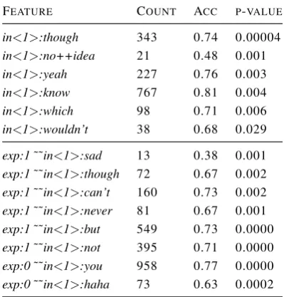
Results of Twitter sentiment analysis with ULM-FiT are shown in Table2. What is worth to note that the model has a problem with positive tweets that contain words of negation or words express-ing sadness or anger by their own (not in a longer context), e.g. “can’t”, “doesn’t”. Examples of such hard cases are: “Don’t hate physics. it is lovely.”, “It doesn’t mean I am angry with him.”.
We performed an additional test with the ULM-FiT model: We trained the model using half of the training set (774,998 text samples) and then found interesting/suspicious features. We added a set of samples (of size 18,009) with “though”
word, then trained a new model (though-model). Additionally, we combine preliminary set with the same additional number (18,009) of random
FEATURE COUNT ACC P-VALUE
in<1>:though 343 0.74 0.00004
in<1>:no++idea 21 0.48 0.001
in<1>:yeah 227 0.76 0.003
in<1>:know 767 0.81 0.004
in<1>:which 98 0.71 0.006
in<1>:wouldn’t 38 0.68 0.029
exp:1˜˜in<1>:sad 13 0.38 0.001
exp:1˜˜in<1>:though 72 0.67 0.002
exp:1˜˜in<1>:can’t 160 0.73 0.002
exp:1˜˜in<1>:never 81 0.67 0.001
exp:1˜˜in<1>:but 549 0.73 0.0000
exp:1˜˜in<1>:not 395 0.71 0.0000
exp:0˜˜in<1>:you 958 0.77 0.0000
[image:6.595.315.515.76.285.2]exp:0˜˜in<1>:haha 73 0.63 0.0002
Table 2: GEval feature listing for classification for sen-timent analysis on Twitter dataset. We used output from model ULMFiT with 0.86 total accuracy on the chosen validation set. “Acc” stands for the average ac-curacy for tweets with a given feature. Labels for pos-itive sentiment are “1”, i.e. in feature names “exp:1” , and for negative sentiment – “0”.
samples (random-model). The “though”-model achieved better accuracy of 85.704% than random and preliminary ones (respectively: 85.383% and 85.558%).
In Figure1, we show the result of LIME method for one data point (sentence) which contains hard features gotten from GEval.
Figure 1: LIME visualisation of influence of tokens on final results. The sentence is marked as positive in gold annotations. GEval hard feature are ”FAIL” and ”which” that generate drop in F1 for the whole test dataset (down to 59% and 71% respectively). They also contributes negatively into this sample.
4.3 Machine translation
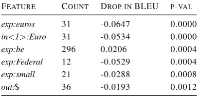
[image:6.595.308.529.510.558.2]than LIUM, using the method described in Sec-tion2.5. In other words, we were looking the spe-cific features for which the best model behaves badly when compared with an inferior model. The interesting features worsening UEDin in compari-son with LIUM are shown in Table3. Inspecting specific sentences we can see a problem that euro currency is translated to pounds, which can be a critical bug in an industry translation system. Obvi-ously, it is very easy to repair with post-processing. However the point is not to overlook the source of model problems, that can be easily and efficiently achieved with GEval.
Other examples of translation problems are “be” which is a very difficult word to translate in various contexts or words like “people” and “Menschen” that meanings varies in different contexts.
FEATURE COUNT DROP INBLEU P-VAL
exp:euros 31 -0.0647 0.0000
in<1>:Euro 31 -0.0534 0.0000
exp:be 296 0.0206 0.0004
exp:Federal 12 -0.0529 0.0004
exp:small 21 -0.0288 0.0008
[image:7.595.78.283.322.421.2]out:$ 36 -0.0193 0.0012
Table 3: Comparison of machine translation models: LIUM and UEDin – features worsening UEDin (WMT-17 new task test data).
4.4 Named entity recognition
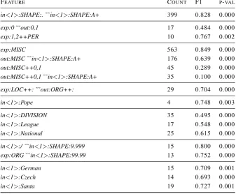
We tested known NER (named entities recogni-tion) models with GEval. Here we report results with FLAIR (Akbik et al.,2018) on CoNLL 2003 dataset (Tjong Kim Sang and De Meulder,2003). We achieved 93.06% F1 score3.
Our test procedure is as follows. We generated GEval listing. Below we explain the findings – GEval features and we show results in Table 4. A few input samples and outputs for the chosen features are presented in Table5. To understand the results we need to bear in mind that output results and annotations (gold standard) are encoded in CoNLL 2003 files as upper-cased named entity class (i.e. LOC, PER, ORG, MISC) and the index in the input sentence, e.g. “LOC:0 PER:7,8”.
3Results reported in authors publication for NER models
on original CoNLL 2003 test set is 93.07%. This result was not achieved with the current version of the library. See the discussion at (Flair,2018).
A few of our finding are presented here (in the Table 4, the relevant rows are listed in the same order):
• upper-cased texts are difficult for the model, e.g. features: in<1>:SHAPE:A+
˜˜in<1>:SHAPE:. (word written in upper case combined with a punctuation mark, i.e. not a header);
• there is a problem when named entity is ex-pected at the beginning of sentence, e.g. exp:0
˜˜out:0,1orexp:1,2++PER. It means that a named
entity was expected just for the first word, but was wrongly marked by the ML model for the first two words);
• there is a problem with MISC class, especially in upper-cased texts and at the beginning of texts, e.g. features: out:MISC
˜˜in<1>:SHAPE:A+; out:MISC++0,1;
out:MISC++0,1˜˜in<1>:SHAPE:A+;
• localization and organization classes are quite often mixed, e.g.exp:LOC++:˜˜out:ORG++:;
• a role of a person is sometimes mixed with the person name and in such cases there is a problem with annotation consistency between train and test dataset, e.g.in<1>:Pope;
• also part of organization names that also are common words are sometimes misannotated or not recognized by the model, e.g.in<1>:League;
in<1>:National;in<1>:DIVISION;
• numbers are hard for the model – numbers for dates, e.g. in<1>:/ ˜˜in<1>:SHAPE:9.999;
exp:ORG˜˜in<1>:SHAPE:99.99.
• and there are many particular cases that are worth looking into, e.g. country names that are might be adjectives as well: in<1>:German;
in<1>:Czech.
5 Conclusions
FEATURE COUNT F1 P-VAL
in<1>:SHAPE:.˜˜in<1>:SHAPE:A+ 399 0.828 0.000
exp:0˜˜out:0,1 17 0.484 0.000
exp:1,2++PER 10 0.767 0.002
exp:MISC 563 0.849 0.000
out:MISC˜˜in<1>:SHAPE:A+ 176 0.639 0.000
out:MISC++0,1 45 0.289 0.000
out:MISC++0,1˜˜in<1>:SHAPE:A+ 35 0.100 0.000
exp:LOC++:˜˜out:ORG++: 29 0.704 0.000
in<1>:Pope 4 0.748 0.003
in<1>:DIVISION 35 0.495 0.000
in<1>:League 17 0.548 0.000
in<1>:National 25 0.615 0.000
in<1>:/˜˜in<1>:SHAPE:9.999 15 0.800 0.000
exp:ORG˜˜in<1>:SHAPE:99.99 13 0.752 0.000
in<1>:German 15 0.709 0.001
in<1>:Czech 14 0.693 0.000
[image:8.595.129.467.81.359.2]in<1>:Santa 19 0.727 0.001
Table 4: Named entity recognition on CoNLL 2003 test dataset with FLAIR model (92.36% for the whole test set).
FEATURE& EXAMPLES GOLD STANDARD ANNOTATIONS& MODEL OUTPUTS
in<1>:National
Peters left a meeting between NZ First and National negotia-tors...
GOLD: ORG:NZ First, ORG:National; OUTPUT: ORG:NZ First and National
in<1>:SHAPE:(
1. United States III ( Brian Shimer , ... ) one; GOLD: ORG:United States III; OUTPUT: LOC:United States
in<1>:Santa
German Santa in bank nearly gets arrested . GOLD: MISC:German PER:Santa; OUTPUT:
MISC:German Santa
Table 5: Named entity recognition on CoNLL 2003 – items from the dataset for features extracted and shown in Table4.
Acknowledgements
The authors would like to acknowledge the support the project conducted by Applica.ai has received as being co-financed by the European Regional Development Fund (POIR.01.01.01-00-0144/17-00).
References
Shared task: Machine translation of news, emnlp wmt 2017.
A. Adadi and M. Berrada. 2018. Peeking inside the
black-box: A survey on explainable artificial intelli-gence (xai).IEEE Access, 6:52138–52160.
Alan Akbik, Duncan Blythe, and Roland Vollgraf. 2018. Contextual string embeddings for sequence labeling. InCOLING 2018, 27th International Con-ference on Computational Linguistics, pages 1638– 1649.
David Jean Biau, Brigitte M. Jolles, and Rapha¨el Porcher. 2010. P value and the theory of hypoth-esis testing: An explanation for new researchers. 468(3):885 – 892.
[image:8.595.71.522.397.531.2]Probabilistic Methods in Economics, volume 809 of Studies in Computational Intelligence, pages 22–44. Springer International Publishing.
Edmund. J. Burr. 1960. The distribution of Kendall’s score S for a pair of tied rankings. Biometrika, 47(1-2):151–171.
Jianbo Chen, Le Song, Martin J Wainwright, and Michael I Jordan. 2018. Learning to explain: An information-theoretic perspective on model interpre-tation.
Mengnan Du, Ninghao Liu, and Xia Hu. 2018. Tech-niques for interpretable machine learning. CoRR, abs/1808.00033.
Flair. 2018.Flair repository (issue 206 and 390).
Mercedes Garc´ıa-Mart´ınez, Ozan Caglayan, Walid Aransa, Adrien Bardet, Fethi Bougares, and Lo¨ıc Barrault. 2017. Lium machine translation systems for wmt17 news translation task. In Proceedings of the Second Conference on Machine Translation, pages 288–295. Association for Computational Lin-guistics.
A. Go, R. Bhayani, and L. Huang. 2009. Twitter senti-ment classification using distant supervision.
Filip Grali´nski, Rafał Jaworski, Łukasz Borchmann, and Piotr Wierzcho´n. 2016. Gonito.net - Open Plat-form for Research Competition, Cooperation and Reproducibility. InProceedings of the 4REAL Work-shop, pages 13–20.
Riccardo Guidotti, Anna Monreale, Salvatore Ruggieri, Franco Turini, Fosca Giannotti, and Dino Pedreschi. 2018.A survey of methods for explaining black box models.ACM Comput. Surv., 51(5):93:1–93:42.
Jeremy Howard and Sebastian Ruder. 2018. Universal language model fine-tuning for text classification.
Maurice G. Kendall. 1938. A new measure of rank cor-relation. Biometrika, 30(1/2):81–93.
Ron Kohavi and Roger Longbotham. 2017. Online Controlled Experiments and A/B Testing, pages 922– 929. Springer US, Boston, MA.
Courtney Napoles, Keisuke Sakaguchi, Matt Post, and Joel Tetreault. 2015. Ground truth for grammati-cal error correction metrics. InProceedings of the 53rd Annual Meeting of the Association for Compu-tational Linguistics and the 7th International Joint Conference on Natural Language Processing (Vol-ume 2: Short Papers), vol(Vol-ume 2, pages 588–593.
Kishore Papineni, Salim Roukos, Todd Ward, and Wei-Jing Zhu. 2002. Bleu: a method for automatic eval-uation of machine translation. In Proceedings of the 40th annual meeting on association for compu-tational linguistics, pages 311–318. Association for Computational Linguistics.
Matt Post. 2018. A call for clarity in reporting BLEU scores.CoRR, abs/1804.08771.
Rico Sennrich, Barry Haddow, and Alexandra Birch. 2016. Edinburgh neural machine translation sys-tems for wmt 16. InProceedings of the First Con-ference on Machine Translation: Volume 2, Shared Task Papers, pages 371–376. Association for Com-putational Linguistics.
Erik F. Tjong Kim Sang and Fien De Meulder. 2003. Introduction to the conll-2003 shared task: Language-independent named entity recognition. In Proceedings of the Seventh Conference on Natural Language Learning at HLT-NAACL 2003 - Volume 4, CONLL ’03, pages 142–147, Stroudsburg, PA, USA. Association for Computational Linguistics.
Marco Tulio Ribeiro, Sameer Singh, and Carlos Guestri. 2016. Model-agnostic interpretability of machine learning. In Proceedings of the Inter-national Conference on Machine Learning, Work-shop on Human Interpretability in Machine Learn-ing (WHI / ICML 2016), Stanford, CA. Morgan Kaufmann.
Frank Wilcoxon. 1945. Individual comparisons by ranking methods.Biometrics Bulletin, 1(6):80–83.