Learning the Dyck Language with Attention based Seq2Seq Models

138

Learning the Dyck Language with Attention-based Seq2Seq Models

Xiang Yu, Ngoc Thang Vu, Jonas Kuhn

Institute for Natural Language Processing (IMS) Universit¨at Stuttgart, Germany

{xiangyu,thangvu,jonas}@ims.uni-stuttgart.de

Abstract

The generalized Dyck language has been used to analyze the ability of Recurrent Neural Net-works (RNNs) to learn context-free grammars (CFGs). Recent studies draw conflicting con-clusions on their performance, especially re-garding the generalizability of the models with respect to the depth of recursion. In this paper, we revisit several common models and experi-mental settings, discuss the potential problems of the tasks and analyses. Furthermore, we ex-plore the use of attention mechanisms within the seq2seq framework to learn the Dyck lan-guage, which could compensate for the limited encoding ability of RNNs. Our findings reveal that attention mechanisms still cannot truly generalize over the recursion depth, although they perform much better than other models on the closing bracket tagging task. Moreover, this also suggests that this commonly used task is not sufficient to test a model’s understanding of CFGs.

1 Introduction

The generalized Dyck language has been a testbed for several research on the ability of Recurrent Neural Networks (RNNs), in particular the Long Short-term Memory model (LSTM) ( Hochre-iter and Schmidhuber, 1997), to learn context-free grammars. It consists of strings with bal-anced pairs of brackets of different types, e.g.,

“[ < > ] [ ] < [ ] >”. Recognizing the

generalized Dyck language is considered to be more difficult than anbn as tested in Gers and Schmidhuber (2001), since it cannot be simply solved by counting. Rather, the model has to remember the sequence of different (unclosed) brackets.

Among the recent studies, Sennhauser and Berwick (2018) analyze the generalizability of LSTMs to learn the generalized Dyck language

with two pairs of brackets, and conclude that the model cannot learn the underlying grammar rules. In contrast,Skachkova et al.(2018) concludes that the LSTM can model the language quite well. Bernardy(2018) experiment with several variants of RNNs, and find that the LSTM works reason-ably well on the given task, but fails to generalize to cases with deeper recursion.

All the aforementioned work explores the abil-ity to “understand” context-free languages with some tagging task similar to language model-ing. In these tasks, the RNN encodes a sequence, which is the prefix of a valid sequence in the lan-guage, and predicts the next possible token either for the last token or for every token. These prob-ing tasks have one thprob-ing in common, namely they predict only one token, which does not necessarily close the whole sequence, and thus are not suffi-cient to prove that the model learns the whole se-quence.

In this work, we show that a seq2seq model with attention mechanism not only solves the tagging task, but also generalizes well over unseen depths. While it appears to have “understood” the Dyck language, under closer inspection, it fails to com-plete deeper sequences and only closes the first several brackets correctly, which happens to be the evaluation metric of the tagging task.

2 Related Work

Instead of natural language data, where the correlation between structural and contex-tual/semantic information is difficult to avoid, many analyses with synthetic data have been conducted on RNNs since their invention, e.g., handling the XOR problem (Elman, 1990), the context-free language anbn and context-sensitive language anbncn (Gers and Schmidhuber, 2001; Weiss et al.,2018b), and extracting finite-state au-tomata (Weiss et al.,2018a).

Among the context-free languages, the general-ized Dyck language is a popular choice since it is simple enough in concept while expressive enough to represent all context-free languages (Chomsky and Sch¨utzenberger,1963).

Skachkova et al.(2018) probes the recognition of the generalized Dyck language in two tasks. The first one is a language modeling task which predicts the next bracket in the actual generated data and measures the perplexity, which compli-cates the evaluation by introducing unnecessary non-determinism. The second task predicts the last closing bracket of a balanced Dyck word, which could be solved with a short-cut. One simply needs to keep a counter for the depth of the sequence, and record the most recent opening bracket each time the counter hits zero. The task is over-simplified by the fact that all the instances are balanced, thus there is no need to memorize anything deeper than the outmost bracket.

Bernardy (2018) and Sennhauser and Berwick (2018) both frame the task as predicting the next valid closing bracket at any position in a Dyck word, which is arguably more difficult to by-pass. Both works also put much emphasis on the generalization over the depth. Comparing to Sennhauser and Berwick(2018), our tagger mod-els, while not perfectly generalizable, perform well above chance level, and the discrepancy be-tween training and testing performance is much smaller. But the general conclusion holds, the RNN-based taggers do not generalize well for the task. Bernardy (2018) reports better results, but they use much shorter sequences (less than 20) where the model has a chance to memorize instead of generalize.

With a different architecture,Deleu and Dureau (2016) uses a Neural Turing Machine (Graves et al.,2014) to recognize the Dyck language. They use the model as an acceptor for the original Dyck language with only one type of bracket pair, which

is much simpler both as a task and as a language. To solve this task, the model only needs to approx-imate a counter, and increment or decrement upon an opening or closing bracket. The LSTM’s abil-ity to approximate a counter machine is discussed inWeiss et al.(2018b).

While all these studies test the RNNs as ac-ceptor (classifier) or transducer (tagger), we also test their ability to decode sequences, which is ar-guably a harder task.

3 Task and Models

The Dyck language consists of strings (a Dyck word) of equal number of opening and closing brackets, and the number of closing brackets is never more than the opening brackets in any pre-fix of the string (a Dyck prepre-fix). The general-ized Dyck language has more than one type of bracket pairs, where all pairs have to be balanced and no crossing of different pairs is allowed. For-mally, the generalized Dyck language is defined asDPwith(oi,ci)∈P, where(oi,ci)are different

bracket pairs. The language can be described by the following grammar:

S→S S S→oiSci

S→oici

We adopt the commonly used tagging task, in which the model has to predict the next valid clos-ing bracket given any Dyck prefix shorter than 100. Note that this differs from the language mod-eling task, since the target is not from the ac-tual, stochastic dataset, but an unambiguous clos-ing bracket. If the prefix is already a balanced Dyck word, then the target is a special symbol ‘$’, which also makes it a recognition task for balanced Dyck words.

We compare four models with different archi-tectures and different training objectives, but the main target is the same. All models have the same encoder architecture, a one-layer bidirec-tional LSTM with 50 hidden units, and only differ in the decoder.

The first model tagger-last predicts the tar-get with a simple linear transformation from the LSTM state of the last token.

The second model tagger-all has exactly the same architecture, but it is trained to predict a clos-ing bracket after every token in the sequence. The

evalua-tion and comparison, while the rest can be viewed as an auxiliary task.

The third model generator-simplefollows the common seq2seq architecture (Sutskever et al., 2014). It generates a sequence of closing brack-ets to eagerly complete the Dyck prefix into a bal-anced Dyck word, and the generation stops when the ‘$’ symbol is predicted. For this model, the

first generated bracket is the main target and the rest is the auxiliary task.

The fourth model generator-attention aug-ments the decoder with the attention mechanism (Bahdanau et al.,2014). It uses thegeneral vari-ant of attention (Luong et al.,2015):

score ht,hs

=h>_t Wahs

whereht denotes the decoder state, hsdenotes all

encoder states, andWais the model parameter.

All the models are trained with the Adam opti-mizer (Kingma and Ba,2014) with the default pa-rameters in the Dynet library (Neubig et al.,2017). The generator models are trained with the stan-dard teacher forcing method, since there is only one correct target sequence and the model is eval-uated on exact match.

No special tuning of hyperparameters is per-formed, and we do not use mini-batch or dropout, since the training is fast and stable enough.1

4 Experiments

4.1 Data

We largely adopt the experimental settings and ter-minologies inSennhauser and Berwick(2018) for comparison.

The dataset we use in the experiment consists of 1 million instances, each one is a Dyck pre-fix of length up to 100 with two different types of brackets(‘[’, ‘]’ and ‘<’, ‘>’). The instances are sampled proportional to their lengths, i.e., there are twice as many instances of length 20 as in-stances of length 10. We have a preference for longer sequences, since they represent the more difficult cases.

The instances are generated in the following procedure: Until the desired length is reached, generate a random opening bracket with a branch-ing probability p or a valid closing bracket with

1_{The code as well as the dataset are available at the first}

author’s homepage.

distance = 8

embedded depth = 3 depth = 2 [

<

<

[

[ [

< [ [ ]

> >

>

] ]

] [ < < [ ] > > [ [ < > [ [ ] ] ]

Figure 1: A visual representation of a Dyck prefix and the property values of the target token (the last ‘]’).

probability 1−p. If the current sequence is bal-anced (no unclosed brackets), then generating a random opening bracket is the only option.

This generation procedure is similar to Skachkova et al. (2018), except that we do not stop generation once the sequence is balanced, instead we generate a new opening bracket and continue until the desired length is reached. Also, the generated sequence is not necessarily a Dyck word, but a prefix of it.

We adopt the following properties from Sennhauser and Berwick (2018) to describe the Dyck prefixes:

• depthis the number of unclosed brackets;

• embedded depth is the maximum depth be-tween the target closing bracket and the cor-responding opening bracket, which is also called therelevant clause;

• distanceis the number of tokens in the rele-vant clause.

Intuitively, embedded depth correlates with dis-tance, since the deeper the relevant clause, the longer the distance between the outermost brack-ets. Figure1illustrates an example of a Dyck pre-fix and the properties of the final target token.

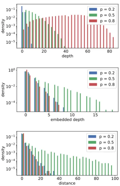
The branching probability pcontrols the distri-bution of the these properties in the samples, the higher its value, the deeper the string is likely to be. Figure 2 visualizes the distribution of each property value when selecting different p in the generation. We choose p=0.5 since it generates enough samples of reasonably high values of both depth and embedded depth/distance.

0 20 40 60 80 depth

10−5 10−4 10−3 10−2 10−1

de

nsi

ty

p = 0.2 p = 0.5 p = 0.8

0 5 10 15

embedded depth 10−4

10−2 100

de

nsi

ty

p = 0.2 p = 0.5 p = 0.8

0 20 40 60 80 100

distance 10−5

10−4 10−3 10−2 10−1

de

nsi

ty

p = 0.2 p = 0.5 p = 0.8

Figure 2: Distribution of depth, embedded depth, and

distance of the dataset with different p values. The

plots are on logarithmic scales.

Generating identical longer sequences is practi-cally impossible, since the number of generalized Dyck prefixes of length 100 is orders of magni-tudes larger than the dataset2.

The main target of an instance is the matching closing bracket given the prefix, and if the prefix is balanced, a special symbol ‘$’ is the target. To avoid inflated results in the evaluation, we ignore the easy cases where the last token is an opening bracket, since the target is simply the correspond-ing closcorrespond-ing bracket, and does not require further memory to make the correct prediction. However, we do not remove these cases from training, since it is still a correct behavior to learn, albeit very simple.

We split the dataset into training set and test set in different ways. In the in-domain setting, the dataset is equally split into training set and test set, and both sets have roughly the same distribution of

2_{The exact number is beyond the scope of this work, but}

a simple lower-bound would be the 50-th Catalan number (greater than 1027_{), which is the number of Dyck words of}

length 100 with only one pair of brackets.

the property values. In the out-of-domain setting, where we test the generalization of the models, we sort the dataset by the respective maximum prop-erty values of the whole sequence, and train on the instances where the value is smaller than 1₃ of the maximum in the dataset, i.e., we test the general-ization on up to three times the training depth.

Note that the selection criteria is the maximum

value over the whole sequence, not just of the final target. This is a much stricter condition than in Sennhauser and Berwick(2018), since the encoder would never see a training instance that is too deep at any step. For example in Figure 1, the target depth is 2, while the maximum depth is 5.

We test the models on the development set (a held-out portion of the training set) after every 10000 training steps, and stop training if the per-formance do not improve 5 times in a row. Most of the time, the training terminates before even it-erating through the training data once.

Due to the stochastic nature of neural networks, we report the results of each model/condition from the average of 10 runs with different random seeds.

4.2 In-Domain Results

target all-tags completion

tagger-last 96.4% 98.8% -tagger-all 98.7% 99.8% -gen-simple 96.3% - 82.1% gen-attn 99.9% - 97.8%

Table 1: Average accuracy of the models in differ-ent evaluations in the in-domain setting. In the three

columns,targetmeasures the accuracy of the main

tar-get,all-tagmeasures the average accuracy of

predict-ing the next bracket for all tokens, completion

mea-sures the exact match of closing all the brackets. All results are averaged from 10 runs.

The average results of the in-domain experi-ments are shown in Table 1. All the models are evaluated on the main target of the same test set (the first column), and the tagger models are addi-tionally evaluated on predicting the target for ev-ery token in the sequence (the second column).

Overall, all models perform reasonably well, whiletagger-allperforms better thantagger-last

itera-in-domain out-of-domain

tagger

-last

0 10 20 30 40

depth 0.0 0.2 0.4 er ro r ra te

0 10 20 30 40

depth 0.0 0.2 0.4 er ro r ra te tagger -all

0 10 20 30 40

depth 0.0 0.2 0.4 er ro r ra te

0 10 20 30 40

depth 0.0 0.2 0.4 er ro r ra te gen-simple

0 10 20 30 40

depth 0.0 0.2 0.4 er ro r ra te

0 10 20 30 40

depth 0.0 0.2 0.4 er ro r ra te gen-attn

0 10 20 30 40

depth 0.0 0.2 0.4 er ro r ra te

0 10 20 30 40

depth 0.0 0.2 0.4 er ro r ra te

Figure 3: Errors of each model in the in-domain vs. out-of-domain setting for thedepthproperty.

in-domain out-of-domain

tagger

-last

0 5 10 15 20

embeded depth 0.0 0.2 0.4 err or rat e

0 5 10 15 20

embeded depth 0.0 0.2 0.4 err or rat e tagger -all

0 5 10 15 20

embeded depth 0.0 0.2 0.4 err or rat e

0 5 10 15 20

embeded depth 0.0 0.2 0.4 err or rat e gen-simple

0 5 _{embeded depth}10 15 20 0.0 0.2 0.4 err or rat e

0 5 _{embeded depth}10 15 20 0.0 0.2 0.4 err or rat e gen-attn

0 5 10 15 20

embeded depth 0.0 0.2 0.4 err or rat e

0 5 10 15 20

embeded depth 0.0 0.2 0.4 err or rat e

Figure 4: Errors of each model in the in-domain vs. out-of-domain setting for theembedded depthproperty.

tion, training on multiple targets in one sequence is still beneficial. We hypothesize that it is because predicting for all tokens in one sequence requires the model to encode the information more consis-tently. However, more experiments are needed to confirm the hypothesis. Both models have higher accuracies on all tags than the last tag, presum-ably because the average prefix depth and embed-ded depth on all tags are lower than that of the last

tag, which are easier to predict.

in-domain out-of-domain

tagger

-last

0 20 40 60 80 100

distance 0.0

0.2 0.4

er

ro

r

ra

te

0 20 40 60 80 100

distance 0.0

0.2 0.4

er

ro

r

ra

te

tagger

-all

0 20 40 60 80 100

distance 0.0

0.2 0.4

er

ro

r

ra

te

0 20 40 60 80 100

distance 0.0

0.2 0.4

er

ro

r

ra

te

gen-simple

0 20 40 60 80 100

distance 0.0

0.2 0.4

er

ro

r

ra

te

0 20 40 60 80 100

distance 0.0

0.2 0.4

er

ro

r

ra

te

gen-attn

0 20 40 60 80 100

distance 0.0

0.2 0.4

er

ro

r

ra

te

0 20 40 60 80 100

distance 0.0

0.2 0.4

er

ro

r

ra

te

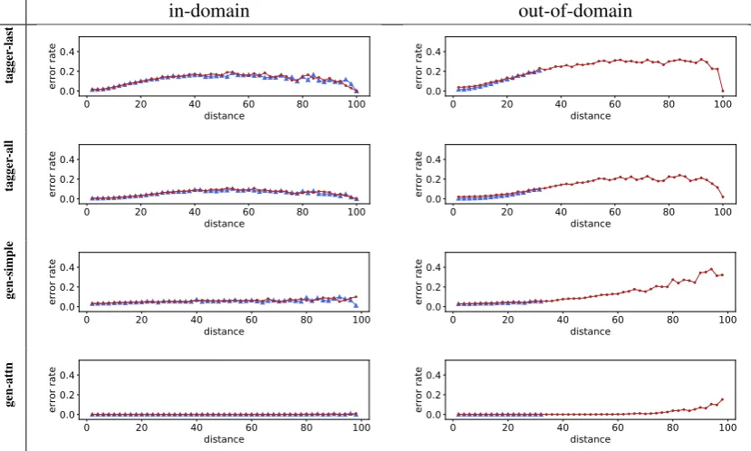
Figure 5: Errors of each model in the in-domain vs. out-of-domain setting for thedistanceproperty.

Finally, when the generator model is equipped with attention, it achieves almost perfect perfor-mance even for the exact completion.

4.3 Generalization

The detailed results of the four models in the in-domain vs. out-of-in-domain settings according to different properties (depth, embedded depth, and

distance) are shown in Figure3,4, and5, respec-tively. We remove the noisy points from the plot when there are less than 10 cases. The chance level of the error rate lies slightly over 0.5, since the two closing brackets are equiprobable and in about 10% of the case the target is ‘$’ (a balanced Dyck word). In each group of plots, the ones on the left show the in-domain setting, on the right the out-of-domain setting. The four rows are the four models: tagger-last, tagger-all, generator-simple, and generator-attention. In each figure, the blue triangles are the training error rates, and the red dots the test error rates.

It is evident from the in-domain experiments on the left side of the plots that all the models gen-eralize well in the in-domain setting (but not nec-essarily performing well), since the training errors (blue triangles) and test errors (red dots) align very closely. This means that all the models are not simply memorizing the training data.

The more interesting case is the out-of-domain condition, where we test the models on sequences

up to three times as deep as the training data. Among the two weaker models,generator-simple

is very sensitive to the depth, while tagger-last

is more sensitive to theembedded depth and dis-tance. This means that the two models are prone to different problems, although having comparable performance.

Note that in the out-of-domain setting fordepth, the first three models have higher test error rate even for smaller depth. Recall that we split the dataset by the maximum depth of the sequence, while reporting the error by the depth of the cur-rent target, which means that they are tested on se-quences that have deeper recursion at some point, and the encoder can not recover from it. The only exception isgenerator-attention, which is not af-fected by this situation. Furthermore, this model generalize well in all conditions.

4.4 Tasks Revisited

0 10 20 30 40 depth

0.0 0.2 0.4

er

ro

r

ra

te

(a) Tagging error rate.

0 10 20 30 40

depth 0.0

0.5 1.0

er

ro

r

ra

te

(b) Completion error rate.

Figure 6: Error rates of the tagging and completion

tasks of thegenerator-attentionmodel in the

out-of-domain setting.

of a Dyck word (Skachkova et al.,2018) also only requires counting the depth and keeping track of the most recent opening bracket of depth 0.

In our tagging task, the generator-simple

model performs very poorly when the depth is high. This is because the model has to memo-rize all the opening brackets, in order to generate the full closing sequences. Apparently, the RNN encoder alone is not capable of memorizing the whole sequence (even in the in-domain condition), and the noise in the memory causes the decoder unable to correctly predict even the first bracket, which is the main evaluation target.

The generator-attention model consistently performs better, since it avoids compressing the whole sequence into a fixed sized vector. Instead, it keeps all the input tokens as individual (contex-tualized) vectors, and use the attention mechanism to find out the corresponding opening bracket, and the decoder only needs to map the attended open-ing bracket into the correspondopen-ing closopen-ing one.

Figure 6 shows the tagging error rate and the completion (exact match) error rate of the same

generator-attention model in the out-of-domain setting. The completion performance deteriorate very rapidly beyond the depth that the model is trained on, while the tagging performance seems quite stable. This contrast clearly demonstrates that the tagging task is inadequate to test the RNN’s ability of modeling CFGs.

4.5 Attention

We have seen that even the best performing

generator-attention model cannot generalize in

(a) depth = 10. (b) depth = 20.

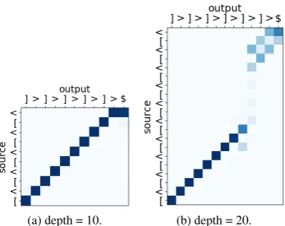
Figure 7: Attention matrices of a model trained on data with maximum depth of 10 and tested on sequences with depths of 10 and 20.

the out-of-domain condition to complete the full closing bracket sequence, although it is able to predict the first bracket correctly.

To identify the problem, Figure7visualizes the attention matrices in the out-of-domain setting, in which we take a generator-attention model trained on the dataset with maximum depth of 10, and test on the sequences with depth of 10 and 20. While the attention alignment seems perfect for the sequence of depth 10, it gets blurry on a deeper sequence. The first 9 output brackets are still correctly aligned and predicted, the attention then jumps over to the beginning of the source and finishes the generation. This explains the sudden deterioration of completion performance in Fig-ure6b, since almost all instances that are too deep are closed prematurely.

This problem, however, is not manifested in the tagging task as in Figure 6a, since it only mea-sures whether the first generated bracket is correct, while the generator only starts to make mistakes after a certain number of steps.

4.6 Equivalence Test

As human, while performing the tagging and completion tasks (as well as many other tasks mentioned before) on the generalized Dyck lan-guage, one can utilize an important property to simplify the task, namely the equivalence of different prefixes. For example, two prefixes

“[ < < [ < < [ ] > >” and “[ < < [”

(a) tagger-last (b) tagger-all

(c) recurrent-simple (d) recurrent-attention

Figure 8: Equivalence test of four models.

similar representation for the two prefixes.

We thus design an experiment to test whether our different models are capable of realize such equivalence, and how well it holds under different conditions, namely the depth and embedded depth of the prefix. We construct the dataset by concate-nating an open prefix ([ < < [) to a balanced clause (< < [ ] > >) of different lengths, and measure the L2-norm of the distance of the en-coder LSTM states after reading the open prefix and the balanced clause. Ideally the two states should be very similar, thus the L2-distance close to 0. We randomly generate open prefixes up to length 40, and balanced clauses also up to 40, which correspond to the maximum depth of 40 and embedded depth of 20. We take the in-domain models which have been trained on instances up to these maximum values, but not necessarily the combination of both maximums. For each model, we plot the average L2-distance of 100 samples

for each combination.

Figure 8 shows the results, where lighter cells means two equivalent prefixes have more similar representations. Similar to the main task result, the tagger-last model shows the worst ability to capture the equivalence. Both tagger models are insensitive to the depth and sensitive to the em-bedded depth, which also agrees with the results in Figure4.

The generator models clearly capture the equiv-alence better. However, we observe that the L2-distance at higher depth is slightly smaller, while Figure 3 has shown that recurrent-simple per-forms worse at higher depth. This suggests that the representation at deeper recursion may be sim-ilar but contains only noisy information, which re-quires further investigation in the future work.

5 Conclusion

In this work, we revisit the tasks based on the Dyck language to probe the ability and limitation of RNNs to encode context-free grammars.

We argue that the bracket tagging task is insuf-ficient to prove the ability or expose the limitation of a model, while the bracket completion task has higher requirement as a test. Seq2seq models out-perform the tagger models in the tagging task, but still fail to generalize in the completion task. The failure is especially apparent when visualizing the model’s attention. We also conduct analysis on the RNN’s representation of equivalent prefixes of dif-ferent prefix depth and embedded depth.

Our results suggest that the RNNs can not truly model CFGs, even when powered by the attention mechanism. However, the seq2seq model with at-tention is still a good approximation and fully ca-pable of dealing with recursions as deep as it is trained on.

As future work, we plan to further investigate the open questions in our experiments, especially regarding the attention alignment and equivalence test. Furthermore, the equivalence property could be used not only as a test for the representation, but also as an auxiliary task to enforce better encoding of the RNN.

6 Acknowledgments

References

Dzmitry Bahdanau, Kyunghyun Cho, and Yoshua

Ben-gio. 2014. Neural machine translation by jointly

learning to align and translate. arXiv preprint

arXiv:1409.0473.

Jean-Philippe Bernardy. 2018. Can recurrent neural

networks learn nested recursion? LiLT (Linguistic

Issues in Language Technology), 16(1).

Noam Chomsky and Marcel P Sch¨utzenberger. 1963. The algebraic theory of context-free languages. In

Studies in Logic and the Foundations of

Mathemat-ics, volume 35, pages 118–161. Elsevier.

Tristan Deleu and Joseph Dureau. 2016. Learning

operations on a stack with neural turing machines.

arXiv preprint arXiv:1612.00827.

Jeffrey L Elman. 1990. Finding structure in time.

Cog-nitive science, 14(2):179–211.

Felix A Gers and E Schmidhuber. 2001. LSTM recur-rent networks learn simple free and

context-sensitive languages. IEEE Transactions on Neural

Networks, 12(6):1333–1340.

Alex Graves, Greg Wayne, and Ivo Danihelka.

2014. Neural turing machines. arXiv preprint

arXiv:1410.5401.

Kristina Gulordava, Piotr Bojanowski, Edouard Grave,

Tal Linzen, and Marco Baroni. 2018. Colorless

green recurrent networks dream hierarchically. In

Proceedings of the 2018 Conference of the North American Chapter of the Association for Computa-tional Linguistics: Human Language Technologies, Volume 1 (Long Papers), pages 1195–1205, New Orleans, Louisiana. Association for Computational Linguistics.

Marc D Hauser, Noam Chomsky, and W Tecumseh

Fitch. 2002. The faculty of language: what is

it, who has it, and how did it evolve? science,

298(5598):1569–1579.

Sepp Hochreiter and J¨urgen Schmidhuber. 1997.

Long short-term memory. Neural computation,

9(8):1735–1780.

Diederik P Kingma and Jimmy Ba. 2014. Adam: A

method for stochastic optimization. In

Proceed-ings of the 3rd International Conference on Learn-ing Representations (ICLR).

Tal Linzen, Emmanuel Dupoux, and Yoav Goldberg.

2016. Assessing the ability of LSTMs to learn

syntax-sensitive dependencies. Transactions of the

Association for Computational Linguistics, 4:521– 535.

Thang Luong, Hieu Pham, and Christopher D. Man-ning. 2015. Effective approaches to attention-based

neural machine translation. In Proceedings of the

2015 Conference on Empirical Methods in Natural Language Processing, pages 1412–1421. Associa-tion for ComputaAssocia-tional Linguistics.

Graham Neubig, Chris Dyer, Yoav Goldberg, Austin Matthews, Waleed Ammar, Antonios Anastasopou-los, Miguel Ballesteros, David Chiang, Daniel Clothiaux, Trevor Cohn, Kevin Duh, Manaal Faruqui, Cynthia Gan, Dan Garrette, Yangfeng Ji, Lingpeng Kong, Adhiguna Kuncoro, Gaurav Ku-mar, Chaitanya Malaviya, Paul Michel, Yusuke Oda, Matthew Richardson, Naomi Saphra, Swabha

Swayamdipta, and Pengcheng Yin. 2017. Dynet:

The dynamic neural network toolkit. arXiv preprint

arXiv:1701.03980.

Luzi Sennhauser and Robert Berwick. 2018. Evalu-ating the ability of lstms to learn context-free

gram-mars. InProceedings of the 2018 EMNLP Workshop

BlackboxNLP: Analyzing and Interpreting Neural Networks for NLP, pages 115–124.

Natalia Skachkova, Thomas Trost, and Dietrich

Klakow. 2018. Closing brackets with recurrent

neu-ral networks. In Proceedings of the 2018 EMNLP

Workshop BlackboxNLP: Analyzing and Interpret-ing Neural Networks for NLP, pages 232–239.

Ilya Sutskever, Oriol Vinyals, and Quoc V Le. 2014. Sequence to sequence learning with neural

net-works. InAdvances in neural information

process-ing systems, pages 3104–3112.

Gail Weiss, Yoav Goldberg, and Eran Yahav. 2018a. Extracting automata from recurrent neural networks

using queries and counterexamples. InInternational

Conference on Machine Learning, pages 5244– 5253.

Gail Weiss, Yoav Goldberg, and Eran Yahav. 2018b. On the practical computational power of finite

pre-cision rnns for language recognition. In

Proceed-ings of the 56th Annual Meeting of the Association for Computational Linguistics (Volume 2: Short Pa-pers), volume 2, pages 740–745.

Ethan Wilcox, Roger Levy, Takashi Morita, and

Richard Futrell. 2018. What do RNN Language

Models Learn about Filler–Gap Dependencies? In