Power generation portfolios: A parametric formulation of the efficient frontier

(1)

Munich Personal RePEc Archive

Power generation portfolios: A

parametric formulation of the efficient

frontier

Juárez-Luna, David

Facultad de Economía y Negocios, Universidad Anáhuac México

2 July 2019

Online at

https://mpra.ub.uni-muenchen.de/95983/

(2)

Power generation portfolios: A parametric

formulation of the e¢cient frontier

David Juárez-Luna

July 2, 2019

Abstract

The Portfolio Theory has been extensively used as a planning tool for power generation diversi…cation. However, no one of the existing papers provide a detailed explanation on how the e¢cient frontier of the Power Generation Portfolio (PGP) is costructed. We provide a parametric for-mulation of the e¢cient frontier of PGP of up to 5 _{technologies. The}

analysys takes advantages of the fact that the risk of the PGP is a convex function of the shares of the di¤erent technologies. The parametric for-mulation of the e¢cient frontier of the PGP constitutes a powerfull policy tool for power generation policy-makers.

JEL cassi…cation: D81, G11, Q40, Q49

Keywords: Portfolio, Power Generation, E¢cient Frontier, Risk, NPV.

1 Introduction

The Portfolio Theory, developed by Markowitz (1952), has been extensively used to design plans of power generation diversi…cation (See DeLlano-Paz et al. (2017) for a review). However, no one of the existing papers provide a detailed explanation on how the e¢cient frontier of the Power Generation Port-folio (PGP) is constructed. Without any exception, all of them only present a graph depicting the e¢cient frontier of the corresponding PGP (e.g., Costaet al. (2017), Pinheiro Netoet al. (2017), Adams and Jamasb (2016), Jainet al.

(2014), Cunha and Ferreira (2014), Roqueset al. (2010), Vithayasrichareonet al. (2010a), Vithayasrichareon et al.(2010b), Roques et al. (2008), and Awer-buch and Berger (2003)).

In the present paper we aim to …ll this gap in the literature by providing a parametric formulation of the e¢cient frontier of PGP of up to5 technologies. Following the existing literature, in present analysis thee¢cient frontierrefers to the set of the PGPs that maximize their Expected Net Present Value (ENPV)

(3)

for a given level of risk. This is, the ENPV of ane¢cientPGP can be increased only by increasing its risk (Awerbuch and Berger (2003)). Note that the present analysis could be directly applied to PGP using Levelized Cost of Electricity (LCOE). In such a case, the e¢cient frontier would be a set of PGPs which can yield the lowest expected energy costs at given, acceptable levels of expected risk (Jansenet al. (2006)).

The analysis takes advantages of the fact that the risk of the PGP, given by the Standard Deviation (SD) or the Variance of the NPV, is a convex func-tion of the shares of the di¤erent technologies. First, we obtain the shares of the technologies that guarantee the minimum risk of the NPV of the PGP. We then obtain the maximum ENPV of the PGP. Finally, we construct the e¢cient frontier that corresponds to the parametric equation of the shares of the tech-nologies that link the minimum risk of the NPV of the PGP to its maximum ENPV.

The parametric formulation of the e¢cient frontier of the PGP allows to tackle the problem of energy generation diversi…cation in an economy. Then, it constitutes a powerful policy tool for power generation policy-makers. Actu-ally, it could be applied to portfolios of assets di¤erent than power generation technologies.

The paper also shows that the "portfolio e¤ect" results from the fact that the risk of the PGP is a convex function of the shares of the di¤erent technologies.

As this is a methodological paper, instead of focusing the analysis on PGP of a particular economy, we use hypothetical data. This fact allows to show the scope of the methodology and, at the same time, improves exposition simplicity.

The whole analysis relies on the assumption that the covariances of the NPVs of the di¤erent technologies is zero. Although this is a strong assumption, it leads to gains in tractability and in the scope of the methodology formulated.

To the best of our knowledge, this is the …rst e¤ort to provide a detailed methodology to construct, parametrically, the e¢cient frontier of PGPs.

The paper is organized as follows: In Section 2, we present the preliminaries. Section 3 presents PGP of2technologies. Section 4 presents PGP of3 technolo-gies. PGP of4 technologies are presented in section 5. PGP of 5 technologies are presented in section 6. Section 7 contains the …nal remarks and conclusions. The appendix contains the formal proofs.

2 Preliminaries

(4)

only by increasing its risk. As usual, risk is measured by the SD or, alterna-tively, by the variance. Formally, letXibe the random variable that represents the NPV of technologyi. LetY a random variable describing the NPV of the PGP which is de…ned as follows:

Y =Pn_i₌₁ iXi, with Pn_i=1 i= 1. (1)

Where i2[0;1]represent the share of technologyi. Following result provides the basic tools for the analysis.

Lemma 1 Let Xi a random variable that represents the NPV of technology

i with mean i and variance 2i. Where i 2 [0;1] is the the share of

tech-nology i = 1;2; : : : ; n. Let the PGP be represented by the random variable

Y =Pn_i₌₁ iXi with

Pn

i=1 i= 1. Then

E(Y) =Pn_i₌₁ iE(Xi),

Y =

Pn i=1 i i.

(2)

and

V ar(Y) =E[Y _Y]2,

2

Y =

Pn

i=1 2i 2i +

P P

i<j i j i;j. (3)

where the double summation extends to any valuesi andj , from 1 ton, such thati < j. In addition, i;j =E (Xi i) Xj j is the covariance of the

NPVs of technologiesi andj.

Proof. See pp. 158, Freundet al. (2000).

First result of Lemma 1 indicates that the ENPV of the PGP is a convex sum of the ENPVs of the di¤erent technologies. Following corollary describes such fact.

Corollary 2 Assume that the ENPV of technology 1 is the greatest while the ENPV of technology n is the lowest. Then, it holds that 1 Y n for

Pn

i=1 i= 1.

(5)

shares of the di¤erent technologies are less than one, we expect that the term

P P

i<j i j i;j to be signi…cantly smaller than the term Pni=1 2i 2i. Then, for the following analysis we assume that the covariances among the di¤erent technologies is zero. this is, i;j = 0, for any values i and j , from 1 to n, such that i < j. This assumption leads to a lack of precision in calculating the minimum risk of the PGP. However, such loss is compensated by a gain in tractability and by the scope of the methodology formulated.

Worth noting that the assumption that the covariances of the di¤erent tech-nologies is zero works well when the PGPs use NPVs or LCOSTs of the di¤erent technologies. Nevertheless, such assumption does not seem feasible when the PGPs use capacity factor or installed capacity. In those cases, we can not guar-antee that the termP P_i<j i j i;j will be signi…cantly smaller than the term

Pn

i=1 2i 2i (e.g., Cunha and Ferreira (2014) and Roques et al. (2010)). Then, in such a context, assuming zero covariance amongst the di¤erent technologies would lead to meaningful miscalculations of the risk of the NPV of the PGP.

Then, from now on, the risk of the PGP is described by its SD as follows:

Y =pPn_i=1 2i 2i (4)

Expression (4) and Corollary 2 provide the tools to construct a parametric formulation of thee¢cient frontierof the PGPs.

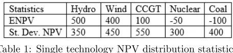
[image:5.612.190.418.515.567.2]

As the main contribution of the paper is the parametric formulation of the ef-…cient frontier, instead of focusing the analysis on PGP of a particular economy, we use hypothetical data. This fact allows to show the scope of the method-ology, and improves exposition simplicity. We consider …ve technologies: 1) Hydro Power Plant (Hydro); 2) Wind Power Plant (Wind); 3) Combined Cy-cle Gas Turbine (CCGT); 4) Advanced Gas-Cooled reactor (NuCy-clear), and; 5) Integrated Gasi…cation Combined Cycle (Coal). Following table present the statistics of the NPV of the di¤erent technologies in USD million.

Table 1: Single technology NPV distribution statistics

Now we have all the building blocks to provide a parametric formulation of the e¢cient frontier of PGPs. We start with portfolios of two technologies.

3 Portfolios of two technologies

(6)

Proposition 3 From expression (4) the SD of the NPV of the PGP of two technologies is given by Y =

p ₂

1 21+ 22 22. Assume that the NPV of

tech-nology2is the less risky. For 1;2= 0, i2[0;1]fori= 1;2, and 1+ 2= 1

it holds that

a) The risk of the NPV of the PGP, given by Y, reaches its global minimum

at

1 2

= 21 1+

2 2

2 2 2 1 b) The minimum risk of the NPV of the PGP is

Y =

q 2 1

2 2 2 1+

2 2 < 2.

Proof. See appendix.

3.1 E¢cient frontier

Following result provides the parametric formulation of the e¢cient frontier for PGP of two technologies.

Proposition 4 Let Y =

p ₂

1 21+ 22 22 be the SD of the NPV of the PGP.

Assume that 1 2, then the following holds:

a) The e¢cient frontiercorresponds to the following parametric equation of the shares of technologies 1 and2,

1

2 = 1 ,

where the parameter is such that 1 df 1. df refers to the

value of that guarantees certain amount of the ENPV of the PGP.

b) The SD in the e¢cient frontier is given by _Y y df . Note that df

1.

c) The maximum ENPV for every corresponding level of risk is given by ( ₁)

y df . Note that df 1. Proof. See appendix.

3.2 Illustrative Portfolios: CCGT-Coal

(7)

1. Following Proposition 3, CCGT corresponds to technology 1 and Coal to technology 2. Then, the shares of the technologies that ensure the minimum risk are

( cc; co) = (0:34595;0:65405).

The minimum risk reached by this PGP is Y = 323:49. And the maxi-mum ENPV for such level of risk is _Y = 30:81.

2. From Proposition 4, the e¢cient frontier corresponds to the following para-metric equation of the shares of the two technologies

cc

co = 1 ,

for0:34595 0:6919. Note that the PGP of CCGT-Coal reaches the maximum ENPV when cc= 1, and Y = cc= 100. However, devoting a share of 100% to CCGT would be very risky in economic and social terms as the SD of the NPV of CCGT is the greatest, cc = 550. In this case the desicion-maker should take a criteria to de…ne the e¢cient frontier. We propose the upper limit of the e¢cient frontier to be df _{= 0}_:₆₉₁₉_. This fact guarantees that the PGP reaches a risk equal to co= 400, the minimum risk of the two technologies.

Note that in this case we might say that CCGT "weakly dominates" the PGP as it has the greatest ENPV which is also relatively risky.1 _On

the other hand, a technology "strongly dominates" a PGP if it has the greatest ENPV and the lowest risk. Roques et al. (2010), Table 4, 2nd scenario, provides a good example where CCGT "strongly dominates" the PGP. However, an economy would face a potential social risk by placing its Power Generation in one single technology. Even in such case, the decision-maker should support Power Generation diversi…cation.

3. The SD in the e¢cient frontier is given by323:49 y 400.

4. The maximum ENPV for every corresponding level of risk is given by

30:81 y 38:38.

1_{See Pinheiro Neto}_{et al.} _{(2017) for clear example where Hydro "weakly dominates" the}

(8)

[image:8.612.136.463.120.577.2]

5. The feasible PGPs of CCGT-Coal are shown in the following …gure:

Figure 1: Feasible PGPs of CCGT-Coal

6. The parameters of the e¢cient frontier are presented in the following …g-ure:

Figure 2: E¢cient Frontier of PGP of CCGT-Coal

4 Portfolios of three technologies

Following result exploits the fact that the SD of the PGP is a convex function of the shares of technologies1, 2, and3,( 1; 2; 3).

Proposition 5 From expression (4) the SD of the NPV of the PGP of three technologies is given by Y =

p ₂

1 21+ 22 22+ 23 23. Assume that the NPV

of technology 2 is the less risky. For 1;2 = 1;3 = 2;3 = 0, i 2 [0;1] for

i= 1;2;3, andP3_i₌₁ i= 1 it holds that

a) The risk of the NPV of the of the PGP, given by Y, reaches its global

minimum at ₀

@ 1₂

3

1

A= 1

jA3j

0

@

2 2 23 2 1 23 2 1 22

1

A,

wherejA3j= 2

1 22+ 21 23+ 22 23.

b) The minimum risk of the NPV of the PGP is

Y =

q 2 1

2 2

2 3 jA3j < 2:

[image:8.612.209.433.146.241.2]

(9)

4.1 E¢cient frontier

Following result provides the parametric formulation of the e¢cient frontier for PGP of three technologies.

p ₂

1 21+ 22 22+ 23 23 the SD of the NPV of the

PGP. Assume that 1 2 3, then following holds:

a) The e¢cient frontiercorresponds to the following parametric equation of the shares of technologies 1,2, and3,

0

@

1 2 3

1

A=

0

@

1+x

1

A,

where the parameter is such that[ 1]

1

1+x df

1. Letxbe given by x =

ln 1 1+ 2

ln_[ 1+ 2]

. df _{refers to the value of} _{that guarantees certain}

amount of the ENPV of the PGP.

1.

c) The maximum ENPV for every corresponding level of risk is given by [ 1]

1 1+x

4.2 Illustrative Portfolios: CCGT-Nuclear-Coal

From Table 1, the corresponding ENPV and variance of the CCGT (cc), Nuclear (nu) and Coal (co) are: cc = 100, nu = 50, co = 100, 2cc = 302500,

2

nu= 90000, and 2co = 160000.

1. Following Proposition 5, CCGT corresponds to technology 1 and Coal to technology 3. Then, the shares of the technologies that ensure the minimum risk are

( cc; nu; co) = (0:15996;0:53763;0:30242).

The minimum risk reached by this PGP is _Y = 219:97. The maximum ENPV for such level of risk is Y = 41:128.

2. From Proposition 6, we obtainx= ln[

0:15996 0:15996+0:53763]

ln[0:15996+0:53763] = 4:089 4and[ 1]

1 1+x ₌

[0:15996]5:08941 _{= 0}_:₆₉₇₅₉_{. Then, the e¢cient frontier corresponds to the}

following parametric equation of the shares of the three technologies

0

@

cc

nu

co

1

A=

0

@

5:0894 5:0894

1

(10)

for0:69759 0:93645. The PGP of CCGT–Nuclear-Coal reaches the maximum ENPV when cc= 1, and Y = cc= 100. In this case, again, CCGT "weakly dominates" the PGP as it has the greatest ENPV which is also the most risky, cc = 550. Then, we propose the upper limit of the e¢cient frontier to be df _{= 0}_:₆₉₁₉_{. This fact guarantees that the} PGP reaches a risk equal to co= 400. Although the ENPV of nuclear is the less risky, it is associated to a lower ENPV of the PGP, Y = 16:17. Then, choosing the upper limit of the e¢cient frontier as df _{= 0}_:₆₉₁₉ allows the PGP to reach a greater ENPV, _y = 54:21, for a considerable risk.

4. The maximum ENPV for every corresponding level of risk is given by

41:128 y 54:21.

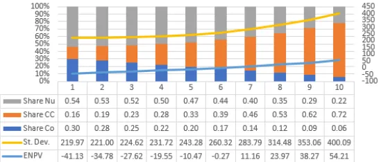
[image:10.612.206.431.343.433.2]

5. The feasible PGPs of CCGT-Nuclear-Coal are shown in the following …g-ure:

Figure 3: Feasible PGP of CCGT–Nuclear-Coal

6. The parameters of the e¢cient frontier are presented in …gure 4.

Figure 4: E¢cient Frontier of PGP of CCGT–Nuclear-Coal

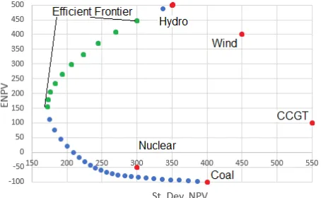
[image:10.612.185.458.489.606.2]

(11)

start by plotting the ENPV and the SD of the NPV of the PGP of CCGT-Nuclear-Coal given as follows

Y =

q

2

cc 2cc+ 2nu 2nu+ (1 cc nu)2 2co,

Y = cc cc+ nu nu+ (1 cc nu) co.

The red surface in Figure 5 corresponds to the risk of the PGP, Y, while the blue plane corresponds to the its ENPV, _Y.

Figure 5: E¢cient Frontier of PGP of CCGT–Nuclear-Coal

The green line in the risk of the PGP depicts the risk of the PGP of CCGT-Coal. The green line in the ENPV of the PGP depicts the ENPV the PGP of CCGT-Coal. Then, placing together the corresponding points of the green lines, we obtain the feasible PGP of CCGT-Coal shown in Figure 1.

The yellow line in the risk of the PGP links the risk of Coal, co, to the risk of CCGT, cc, and the minimum risk of the portfolio, Y. The yellow line in the ENPV of the PGP links the ENPV of Coal, _co, to the ENPV of CCGT, _cc, and the ENPV corresponding to the minimum risk of the portfolio, [ 1]

1 1+x _.

Then, placing together the corresponding points of the yellow lines, we obtain the feasible PGP of CCGT-Nuclear-Coal shown in Figure 3.

The fact that 1 = cc> nu > co = 3 guarantees that: 1) the e¢cient

frontier of the PGP of CCGT-Nuclear-Coal is a segment of the feasible PGP of CCGT-Nuclear-Coal shown in Figure 3; 2) the e¢cient frontier does reach the maximum ENPV for a given level of risk, and; 2) the PGP of CCGT-Nuclear-Coal is less risky than any other PGP containing less than three technologies.

5 Portfolios of four technologies

[image:11.612.180.429.246.370.2]

(12)

Proposition 7 From expression (4) the SD of the NPV of the PGP of four technologies is given by Y =

p ₂

1 21+ 22 22+ 23 23+ 24 24. Assume that the

NPV of technology2is the less risky. Assume that i;j= 0, for any valuesiand

j , from1 to4, such that i < j. If i2[0;1]fori= 1;2;3;4, and

P4

i=1 i= 1

it holds that

a) The risk of the NPV of the PGP, Y, reaches its global minimum at

0 B B @ 1 2 3 4 1 C C A= jA14j

0

B B @

2 2 23 24 2 1 23 24 2 1 22 24 2 1 22 23

1

C C A.

wherejA4j= 2

1 22 23+ 21 22 24+ 21 23 24+ 22 23 24. b) The minimum risk of the NPV of the PGP is

Y = q 2 1 2 2 2 3 2 4 jA4j < 2.

5.1 E¢cient frontier

Following result provides the parametric formulation of the e¢cient frontier for PGP of four technologies.

p ₂

1 21+ 22 22+ 23 23+ 24 24the SD of the NPV of

the portfolio. Assume that the ENPV of technology 1 is the greatest while the ENPV of technology4 is the lowest, then following holds:

a) The e¢cient frontiercorresponds to the following parametric equation of the shares of technologies 1;2;3 and4,

0 B B @ 1 2 3 4 1 C C A= 0 B B @

1+x1

x2 1+x2

1 x2₊ 1+x2

1

C C A,

where the parameter is such that [ 1]

1

1+x₁ df ₁_{. Let} _x1 _and

x2be given byx1=

ln 1 1+ 2

ln_[ 1+ 2]

andx2=

ln 3 3+ 4

ln_[ 1+ 2]

. df _{refers to the value}

of that guarantees certain amount of the ENPV of the PGP.

1.

c) The maximum ENPV for every corresponding level of risk is given by [ ₁]1+1x

1

(13)

5.2 Illustrative Portfolios: Wind-CCGT-Nuclear-Coal

From Table 1, the corresponding ENPV and variance of the Wind (wd), CCGT (cc), Nuclear (nu) and Coal (co) are: _wd = 400, _cc = 100, _nu = 50,

co= 100, 2wd= 202500, 2cc= 302500, 2nu= 90000, and 2co= 160000. 1. Following Proposition 7, Wind corresponds to technology 1 and Coal to

technology 4. Then, the shares of the four technologies that ensure the minimum risk are

( _wd; _cc; _nu; _co) = (0:192 86;0:129 11;0:433 94;0:244 09). The minimum risk reached by this PGP is _Y = 197:62. The maximum ENPV for such level of risk is Y = 43:949.

2. From Proposition 8, we obtain x1 = ln[

0:19286 0:19286+0:12911]

ln[0:19286+0:12911] = 0:45221, x2 = ln[ 0:43394

0:43394+0:24409]

ln[0:19286+0:12911] = 0:39379, and [ 1]

1

1+x₁ _{= [0}_:_19286]

1

1:45221 _{= 0}_:₃₂₁₉₇_.

Then, the e¢cient frontier corresponds to the following parametric equa-tion of the shares of the four technologies

0

B B @

wd

cc

nu

co

1

C C A=

0

B B @

1:45221 1:45221 0:39379 1:39379

1 0:39379₊ 1:39379

1

C C A,

for 0:32197 0:732565. The PGP of Wind-CCGT–Nuclear-Coal reaches the maximum ENPV when wd= 1, and Y = wd= 400. In this case, Wind "weakly dominates" the PGP as it has the greatest ENPV which is also relatively risky, wd= 450. We then propose the upper limit of the e¢cient frontier to be df _{= 0}_:₇₃₂₅₆₅_{. This fact guarantees that} the PGP reaches a risk equal to nu= 300, the minimum risk of the four technologies.

4. The maximum ENPV for every corresponding level of risk is given by43:

949 y 249:26

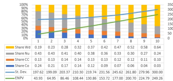
[image:13.612.201.426.559.658.2]

5. The feasible PGPs of Wind-CCGT-Nuclear-Coal are presented in Figure 6.

(14)

6. Following …gure presents the parameters of the e¢cient frontier.

Figure 7: E¢cient Frontier of PGP of Wind-CCGT-Nuclear-Coal

6 Portfolios of …ve technologies

Following result exploits the fact that the SD of the PGP is a convex function of the shares of technologies1, 2,3,4and5,( 1; 2; 3; 4; 5).

Proposition 9 From expression (4) the SD of the NPV of the PGP of …ve technologies is given by Y =

p ₂

1 21+ 22 22+ 23 32+ 24 24+ 25 25. Assume

that the NPV of technology 2 is the less risky. Assume that i;j = 0, for any

values i and j , from 1 to 5, such that i < j. If i 2[0;1]for i= 1;2;3;4;5,

andP5_i₌₁ i= 1it holds that

a) The risk of the NPV of the PGP, Y, reaches its global minimum at

0

B B B B @

1 2 3 4 5

1

C C C C A

= 1

jA5j

0

B B B B @

2 2 23 24 25 2 1 23 24 25 2 1 22 24 25 2 1 22 23 25 2 1 22 23 24

1

C C C C A

.

wherejA5j= 2

1 22 23 24+ 21 22 23 25+ 21 22 42 25+ 21 23 24 52+ 22 23 24 25. b) The minimum risk of the NPV of the PGP is

Y =

q 2 1

2 2

2 3

2 4

2 5 jA5j < 2.

6.1 E¢cient frontier

[image:14.612.175.459.146.280.2]

(15)

p ₂

1 21+ 22 22+ 23 32+ 24 24+ 25 25 the SD of

the NPV of the portfolio. Assume that the ENPV of technology1is the greatest while the ENPV of technology5 is the lowest, then following holds:

a) The e¢cient frontiercorresponds to following parametric equation of the shares of technologies1;2;3;4 and5,

0

B B B B @

1 2 3 4 5

1

C C C C A

=

0

B B B B @

1+x1+x2

1+x2 1+x1+x2

1+x3 1+x2+x3

1+x2 1+x3₊ 1+x2+x3 1

1

C C C C A

.

where the parameter is such that[ 1]

1

1+x_{1 +}x₂ df ₁_{. Let}_x1_,_x2_,

andx3 be given byx1=

ln 1 1+ 2

ln_[1 5]

,x2=

ln 1+ 2 1 ₅

ln_[1 _5] , andx3= ln 3

3+ 4

ln_[1 _5] .

df _{refers to the value of} _{that guarantees certain amount of the ENPV}

of the PGP.

b) The SD in the e¢cient frontier is given by Y y df . Note that df

1.

c) The maximum ENPV for every corresponding level of risk is given by [ 1]

1 1+x_{1 +}x₂

6.2 Illustrative Portfolios:

Hydro-Wind-CCGT-Nuclear-Coal

From Table 1, the corresponding ENPV and variance of the Hydro (hy), Wind (wd), CCGT (cc), Nuclear (nu) and Coal (co) are: hy = 500, wd = 400, cc = 100, nu = 50, co = 100, 2hy = 122500, 2wd = 202500, 2cc =

302500, 2nu= 90 000, and 2co= 160000.

1. To apply Proposition 9, consider that Hydro corresponds to technology1

and Coal to technology5. Then, the shares of the technologies that ensure the minimum risk are

( 1; 2; 3; 4; 5) = (0:24174;0:14624;0:09 7896;0:32904;0:18508).

The minimum risk of this PGP is given by Y = 172:09. And the maxi-mum ENPV for such level of risk is _Y = 154:20.

2. From Proposition 10, we obtain x1 = ln[

0:24174 0:24174+0:14624]

ln[1 0:18508] = 2:3115, x2 = ln_[0:24174+0:14624

1 0:18508 ]

ln[1 0:18508] = 3:6261,x3=

ln_[ 0:097896 0:097896+0:32904]

ln[1 0:18508] = 7:1958, and[ 1]

(16)

[0:241 74]6:93761 = 0_:814 92. Then, the e¢cient frontier corresponds to the

following parametric equation of the shares of the three technologies

0

B B B B @

1 2 3 4 5

1

C C C C A

=

0

B B B B @

6:9376 4:6261 6:9376 8:1958 11:822 4:6261 8:1958₊ 11:822

1

C C C C A

,

for 0:814 92 0:97647. The PGP of Hydro-Wind-CCGT–Nuclear-Coal reaches the maximum ENPV when hy= 1, and Y = hy = 5000. In this case, Hydro "weakly dominates" the PGP. We propose the upper limit of the e¢cient frontier to be df _{= 0}_:₉₇₆₄₇ _{to guarantees that the} PGP reaches a risk equal to nu = 300, the minimum risk of the …ve technologies.

4. The maximum ENPV for every corresponding level of risk is given by154:

20 _y 446:87

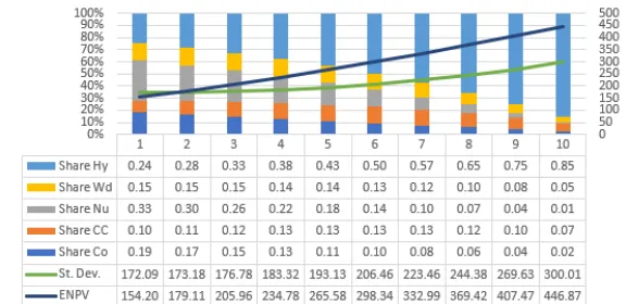
[image:16.612.205.432.396.536.2]

5. Following …gure presents the feasible PGPs of Hydro-Wind-CCGT-Nuclear-Coal

(17)

6. The parameters of the e¢cient frontier are presented in …gure 9.

Figure 9: E¢cient Frontier of PGP of Hydro-Wind-CCGT–Nuclear-Coal

7 Final remarks and conclusions

Present paper tackle the problem of energy generation diversi…cation by pro-viding a parametric formulation of the e¢cient frontier of PGP for up to 5

technologies. Then, the parametric formulation of PGP constitutes a powerful policy tool for power generation policy-makers. Actually, it could be applied to portfolios of assets di¤erent than power generation technologies.

The paper also shows, implicitly, the source of what is called the "portfolio e¤ect": risk reduction attained through diversi…cation. The portfolio e¤ect results from the fact that the risk of the PGP is a convex function of the shares of the di¤erent technologies. Part b) of Propositions 3, 5, 7, and 9 guarantee the existence of the portfolio e¤ect.

From the structure of the paper, it is straight forward to extend the method-ology to obtain the shares of technologies to guarantee the minimum risk of PGP of more than5 technologies. The reader only have to follow the sequence de-picted by Propositions 3, 5, 7, and 9. However, the parametric formulation of the e¢cient frontier of PGPs of more than 5 technologies should be obtained doing the corresponding mathematical proofs. They could be done by following the proof of Propositions 4, 6, 8, and 10.

The complete analysis relies on the assumption that the covariances of the NPV amongst the di¤erent technologies is zero. Depending on computational availability, future research could be extended to verify the actual e¤ect of the correlation of the NPVs on the minimum risk of the portfolio.

[image:17.612.178.466.148.288.2]

(18)

Adams, R., Jamasb, T., 2016. Optimal Power Generation Portfolios: An Application to the UK, Cambridge Working Papers in Economics 1646 / Energy Policy Research Group (EPRG), Working Paper 1620, August, Faculty of Economics, University of Cambridge.

Awerbuch, S., Berger, M., 2003. Applying portfolio Theory to EU Electricity Planning and Policy-Making. IEA/EET Working Paper. IEA. Paris

Costa, O. L.V., Ribeiro, C. O., Rego, E. E., Stern, J. M., Parente, V., Kile-ber, S., 2017. Robust portfolio optimization for electricity planning: An application based on the Brazilian electricity mix. Energy Economics 64: 158–169.

Cunha, J., Ferreira, P., 2014. Designing electricity generation portfolios using the mean-variance approach, Int. J. Sustain. Energy Plan. Manag., 4: 17–30.

DeLlano-Paz, F., Calvo-Silvosa, A., Antelo, S. I., Soares, I., 2017. Energy plan-ning and modern portfolio theory: A review. Renewable and Sustainable Energy Review 77: 636–651.

Freund, J. E., Miller, I, Miller, M., 2000. Estadística matemática con aplica-ciones. Pearson educación.

Jain, S., Roelofs, F., Oosterlee, C. W., 2014. Decision-support tool for assessing future nuclear reactor generation portfolios. Energy Economics 44: 99-112.

Jansen, J.C., Beurskens, L.W.M., Tilburg, X.V., 2006. Application of portfolio analysis to the Dutch generating mix. ECN report C-05-100. Energy research council of Netherlands.

Markowitz H. M., 1952. Portfolio Selection, Journal of Finance, Vol. 7, pp 77-91.

Pinheiro Neto, D., Domingues, E. G., Coimbra, A. P., de Almeida, A. T., Alves, A. J., Calixto W. P., (2017), “Portfolio optimization of renewable energy assets: hydro, wind, and photovoltaic energy in the regulated market in Brazil,” Energy Economics, vol. 64, pp. 238–250, 2017.

Roques, F. A., Hiroux, C., Saguan, M., 2010. Optimal wind power deployment in Europe — A portfolio approach, Energy Policy 38, pp. 3245-3256.

Roques, F. A., Newbery, D. M., Nuttall, W. J., 2008. Fuel mix diversi…cation incentives in liberalized electricity markets: A Mean–Variance Portfolio theory approach, Energy Economics, Volume 30, Issue 4: 1831-1849.

(19)

Vithayasrichareon, P., MacGill, I.F., Wen, F., 2010b. Electricity Generation Portfolio Analysis for Coal, Gas and Nuclear Plant under Future Uncer-tainties. 4th IASTED Asian Conference on Power and Energy Systems

Appendix

Proof of Proposition 3. The SD of the PGP of two technologies is given by Y =

p ₂

1 21+ 22 22. Assume that he NPV of technology2is the less risky.

For 1;2= 0, i 2[0;1]fori= 1;2, and 1+ 2= 1. For tractability, most of

the proof uses the variance of the PGP instead of its SD.

Proof of a) We need to …nd the shares of technologies1 and 2, given by

( 1; 2), that guarantees the minimum risk (variance) of the NPV of the PGP.

For tractability, we start by assuming that 2= 1 1. Then, the variance of

the NPV of the PGP is given by 2

Y = 21 21+ (1 1)2 22. First, we …nd the

critical point. The First Order Conditions (FOC) are:

@ 2

Y

@ 1 = 2 1

2

1+ 2 (1 1) ( 1) 22= 0, (5)

From expression (5) we have

1 21+ 1 22= 22, (6)

which leads to

1=

2 2 2 1+

2

2, (7)

Then, 2 = 1 1=

2 1 2 1+

2

2. The critical point of the variance of the NPV of

the PGP is

( 1; 2) = 21 1+

2 2

2

2; 21 , (8)

To verify that the variance of the NPV of the PGP, 2Y, has a minimum at the critical point( ₁; ₂)we need the Second Order Conditions (SOC):

@2 2

Y

@ 2

1 = 2

2

1+ 22 >0.

Then, the variance 2

Y has a minimum at point( 1; 2). Proof of b)Then, the minimum value of the variance, 2

Y , of the NPV of the PGP is given by

2

Y =_[ 21

1+ 2 2]2

h

2 2

2 ₂ 1+ 21

2 ₂ 2

i

,

2

Y = 2Y =

2 1

2 2 [ 2

1+ 2

2]2 2₂+ 2₁ ,

2

Y =

2 1

2 2 2 1+

2 2 = 2

2 2< 22,

Then

(20)

The NPV of the PGP is less risky than the NPV of the less risky technology.

Proof of Proposition 4. Let Y =

p ₂

1 21+ 22 22the SD of the NPV of the

PGP. From Proposition 3 we know that the risk of the NPV of the PGP, Y, reaches its global minimum at point( 1; 2). Assume that 1 2.To obtain

the parametric formulation of the e¢cient frontier, we write the variance of the portfolio as follows:

2

Y = 2 21+ (1 )

2 2

2, (10)

for 2[0;1]. Note that when = 1, then 2

Y = 21, the variance of the NPV

of the PGP equals the variance of technology 1. This scenario ensures that technology1, which has the greatest ENPV, receives a share of 100%. On the other hand, when = 0, then 2

Y = 22, the variance of the NPV of the PGP

equals the variance of technology2. The latter implies that technology2, which has the lower ENPV, receives a share of 100%. Then, this way of expressing the variance of the NPV of the PGP allows to have portfolios assigning a share of 100% to the technologies with the greater and lower ENPV. To be sure that expression (10) allows to reach the point ( 1; 2) where Y reaches its global minimum, it should hold that

1= , (11)

2= 1 , (12)

Expressions (11) and (12) lead to the fact that the shares of technologies1and

2in this PGPs are given by the following expressions

1= , (13)

2= 1 , (14)

From expressions (13) and (11), the PGP with lowest risk (variance or SD) is given when

= 1. (15)

Now we need to …nd the PGP with the greatest ENPV. The ENPV of the PGP is given by:

Y = 1 1+ 2 2, (16)

substituting expressions (13) and (14) into expression (16) leads to

Y = 1+ (1 ) 2,

it is straight forward to obtain that

d Y

d = 1 2>0,

because of the assumption that 1 2. Then, thePGP reaches its maxi-mum ENPV when = 1, and Y = 1 and 2Y = 21. However, there could

(21)

to choose df _{such that} 2

Y df = 22. In this case df <1. Then, the PGP with maximum ENPV given when = df_{. Then,} _{the e¢cient frontier} is given by expressions (13) and (14) for 1 df. As a consequence, the

SD in the e¢cient frontier is given by _Y y df while the maximum ENPV for every corresponding level of risk is given by ( 1) y df . Note that df

1 and df 1.

Proof of Proposition 5. The SD of the of the NPV of the PGP of three technologies is given by Y =

p ₂

1 21+ 22 22+ 23 23. Assume that the NPV

of technology 2 is the less risky. For 1;2 = 1;3 = 2;3 = 0, i 2 [0;1] for i = 1;2;3, and P3_i=1 i = 1. For tractability, most of the proof uses the variance of the PGP instead of its SD.

Proof of a)We need to …nd the shares of technologies1,2, and3, given by

( 1; 2; 3)that ensures the minimum risk (variance) of the NPV of the PGP.

For tractability, we start by assuming that 3= 1 1 2. Then, the variance

of the NPV of the PGP is given by 2

Y = 21 21+ 22 22+(1 1 2)2 23. First,

we …nd the critical point. The FOC are:

@ 2

Y

@ 1 = 2 1

2

1+ 2 (1 1 2) ( 1) 23= 0, (17)

@ 2

Y

@ 2 = 2 2

2

2+ 2 (1 1 2) ( 1) 23= 0, (18)

from expression (17) we have

1 21+ 23 + 2 23= 23, (19)

1 23+ 2 22+ 23 = 23. (20)

Expressions (19) and (20) lead to the following system of equations

2

1+ 23 23 2

3 22+ 23 1 2 =

2 3 2 3

, (21)

Calculating the inverse of matrixA3=

2

1+ 23 23 2

3 22+ 23

we end up with

1 2 =

1

jA3j

2

2+ 23 23 2

3 21+ 23 2 3 2

3 , (22)

wherejA3j= 2

1 22+ 21 23+ 22 23. Leading to the result 1

2 = 1

jA3j

2 2 23 2

1 23 , (23)

Then, 3= 1 1 2=

2 1

2 2

jA3j. The critical point of the variance of the NPV

of the PGP is

(22)

To verify that the variance of the NPV of the PGP, 2

Y, has a minimum at point( 1; 2; 3)we need the SOC. The Hessian matrix is as follows:

H= 2

2

1+ 23 23 2

3 22+ 23

,

Following the criteria of the leading principal minors of the Hessian matrix, we have

H1= 2 21+ 23 >0: H2= 2jA3j= 2 2

1 22+ 21 23+ 22 23 >0.

The two leading principal minors of the Hessian matrix are positive for any

( 1; 2; 3). Then, the variance of the NPV of the PGP is a convex function of

the shares of the three technologies,( 1; 2; 3). As a consequence, the variance

of the NPV of the PGP, 2

Y, has a global minimum at point( 1; 2; 3), given

by expression (24).

Proof of b) Then, the minimum value of the variance of the NPV of the PGP is

2

Y =[A13]2

h

2 2 23

2 ₂

1+ 21 23 2 ₂

2+ 21 22 2 ₂

3

i

,

2

Y =

2 1

2 2

2 3

[A3]2

2

1 22+ 21 23+ 22 23 , 2

Y =

2 1

2 2

2 3

A3 = 2

2 2< 22,

Then

Y < 2. (25)

The NPV of the PGP is less risky than the NPV of the less risky technology.

p ₂

1 21+ 22 22+ 23 23 the SD of the

NPV. From Proposition 5 we know that the risk of the NPV of the PGP, Y, reaches its global minimum at point( 1; 2; 3). Assume that 1 2 3.To

obtain the parametric formulation of the e¢cient frontier, we write the variance of the portfolio as follows:

2

Y = 2 2 21+ (1 )

2 2

2 + (1 ) 2 2

3, 2

Y = 2 2 21+ 2(1 ) 2 2

2+ (1 ) 2 2

3,

(26)

for ; 2[0;1]. Note that when = = 1, then 2

Y = 21, the variance of the

portfolio equals the variance of technology1. This fact implies that technology

1, which has the greatest ENPV, receives a share of 100%. On the other hand, when = 0, then 2

Y = 23, the variance of the portfolio equals the variance

(23)

the greatest and lowest ENPV. To be sure that expression (26) allows to reach the point( 1; 2; 3), where Y reaches its global minimum, it should hold that

1= , (27)

2= (1 ), (28)

3= (1 ), (29)

from expression (27)

= 1 ₍₃₀₎

substituting expression (30) into expression (28) leads to

= 1

1+ 2, (31)

= 1+ 2. (32)

Assume that

= ( ) = x ₍₃₃₎

to ensure that 2[0;1]for 2[0;1]. Then, from expression (31) and (32) we have

1

1+ 2 = ( 1+ 2)

x .

which leads to

x=

ln 1 1+ 2

ln_[ 1+ 2]

. (34)

Substituting expression (33) into expressions (27), (28), and (29) leads to the fact that the shares of technologies1;2and3 in this portfolio are given by the following expressions

1= = 1+x, (35)

2= (1 ) = 1+x, (36)

3= 1 . (37)

= [ 1]

1

1+x_. (38)

Now we need to fond the PGP with the corresponding greatest ENPV. The ENPV of the PGP is given by

Y = 1 1+ 2 2+ 3 3, (39)

substituting expressions (35), (36), and (37) into expression (39) leads to

(24)

It is straight forward to obtain that

d Y

d = [1 +x] x_[

1 2] + 2 3>0,

because of the assumption that 1 2 3. Then, the PGP reaches its maximum ENPV when = 1, and _Y = 1 and 2Y = 21. However, there

could be an alternative criteria to choose the maximum ENPV of the PGP. For example, if the NPV of technology 2 is the less risky, then, the criteria could be to choose df _{such that} 2

Y df = 22. In this case df <1. Then, the PGP with maximum ENPV is given when = df_{. Then,} _{the e¢cient}

frontieris given by expressions (35), (36), and (37) for[ 1]

1

1+x df_{. As}

a consequence, the SD in the e¢cient frontier is given by _Y y df while the maximum ENPV for every corresponding level of risk is given by

[ 1]

1 1+x

y df . Note that df 1and df 1.

Proof of Proposition 7. The SD of the NPV of the PGP of four technologies is given by Y =

p ₂

1 21+ 22 22+ 23 23+ 24 24. Assume that the NPV of

technology2 is the less risky. If i;j = 0, for any values i andj , from1 to 4, such thati < j. If i2[0;1]fori= 1;2;3;4, andP4_i=1 i= 1. For tractability, most of the proof uses the variance of the PGP instead of its SD.

Proof of a) We need to …nd the shares of technologies1,2,3, and4, given by ( 1; 2; 3; 4), that ensures the minimum risk (variance) of the NPV of the

PGP. For tractability, we start by assuming that 4= 1 1 2 3. Then,

the variance of the NPV of the PGP is given by 2

Y = 21 21+ 22 22+ 23 23+

(1 1 2 3)2 24. First, we …nd the critical point. The FOC are:

@ 2Y

@ 1 = 2 1

2

1+ 2 (1 1 2 3) ( 1) 24= 0, (40)

@ 2

Y

@ 2 = 2 2

2

2+ 2 (1 1 2 3) ( 1) 24= 0, (41)

@ 2

Y

@ 3 = 2 3

2

3+ 2 (1 1 2 3) ( 1) 24= 0, (42)

1 21+ 24 + 2 42+ 3 24= 24, (43)

1 24+ 2 22+ 42 + 3 24= 24, (44)

1 24+ 2 24+ 3 23+ 24 = 24. (45)

Expressions (43), (44), and (45) lead to the following system of equations

2

4

2

1+ 24 24 24 2

4 22+ 24 24 2

4 24 23+ 24

3

5 2

4

1 2 3

3

5=

2

4

2 4 2 4 2 4

3

(25)

2

4

2

1+ 24 24 24 2

4 22+ 24 24 2

4 24 23+ 24

3

5we end

up with 2 6 6 4 1 2 3 3 7 7 5=jA1

4j 2 6 6 4 2

2 23+ 22 24+ 32 24 23 24 22 24 2

3 24 21 23+ 21 24+ 23 24 21 24 2

2 24 21 24 21 22+ 21 24+ 22 24

3 7 7 5 2 6 6 4 2 4 2 4 2 4 3 7 7 5, (47) wherejA4j= 2

1 22 23+ 21 22 24+ 21 23 24+ 22 23 24. The solution is the system

of equations is ₂

4 1₂

3

5= 1

jA4j

2

4

2 2 23 24 2 1 23 24 2 1 22 24

3

5, (48)

Then, 4= 1 1 2 3=

2 1 2 2 2 3

jA4j . The critical point of the variance of the

NPV of the PGP is

( 1; 2; 3; 4) =jA14j

2

2 23 24; 21 23 24; 12 22 24; 21 22 23 . (49)

Y, has a minimum at point( 1; 2; 3; 4)we need the SOC. The Hessian matrix is as follows:

H = 2

2

4

2

1+ 24 24 24 2

4 22+ 24 24 2

4 24 23+ 24

3

5, (50)

H1= 2 21+ 24 >0,

H2= 2

2

1+ 24 24 2

4 22+ 24

= 2 2

1 22+ 21 24+ 22 24 >0, H3= 2jA4j>0.

The three leading principal minors of the Hessian matrix are positive for any

( 1; 2; 3; 4). Then, the variance of the NPV of the PGP is a convex function

of the shares of the four,( 1; 2; 3; 4). As a consequence, the variance of the

NPV of the PGP, 2

Y, has a global minimum at point( 1; 2; 3; 4), given by

expression (49).

Proof of b) Then, the minimum value of the variance of the NPV of the portfolio is

2

Y =

1 [jA4j]2

h

2 2 23 24

2 ₂

1+ 21 23 24 2 ₂

2+ 21 22 24 2 ₂

3+ 21 22 23 2 ₂

4

i

,

2

Y = 2Y =

2 1 2 2 2 3 2 4

(26)

2

Y =

2 1

2 2

2 3

2 4

jA4j = 2 22< 22,

Then

Y < 2. (51)

The NPV of the portfolio is less risky than the NPV of the less risky technology.

p ₂

1 21+ 22 22+ 23 23+ 24 24 the SD

of the NPV. From Proposition 7 we know that Y reaches its global minimum at point( 1; 2; 3; 4). Assume that the ENPV of technology 1is the

great-est while the ENPV of technology 4 is the lowest. To obtain the parametric formulation of the e¢cient frontier, we write the variance of the portfolio as follows:

2

Y = 2

h

2 2

1+ (1 ) 2 2

2

i

+ (1 )2h 2 2

3+ (1 ) 2 2

4

i

,

2

Y = 2 2 21+ 2(1 ) 2 2

2+ (1 ) 2 2 2

3+ (1 ) 2

(1 )2 2 4

(52)

for ; ; 2[0;1]. Note that when = = 1, then 2

Y = 21, the variance of the

portfolio equals the variance of technology1. This fact implies that technology

1, which has the greatest ENPV, receives a share of 100%. On the other hand, when = = 0, then 2

Y = 24, the variance of the portfolio equals the variance

of technology4. Then, technology4, which has the lowest ENPV, receives share of 100%. Then, this formulation of the variance of the NPV of the PGP allows to have portfolios that assign a share of 100% to the technologies with the greatest and lowest ENPV. To be sure that expression (52) allows to reach the point

( ₁; ₂; ₃; ₄)where Y reaches its global minimum, it should holds that

1= , (53)

2= (1 ), (54)

3= (1 ) , (55)

4= (1 ) (1 ), (56)

= 1_, ₍₅₇₎

= 1

1+ 2, (58)

= ₁+ ₂. (59)

From expression (55)

(27)

= 3

3+ 4. (61)

Assume that

= ( ) = x1 ₍₆₂₎

= ( ) = x2 ₍₆₃₎

to ensure that 2 [0;1] and 2 [0;1] for 2 [0;1]. Then, substituting expressions (58) and (59) into expression (62) he have

1

1+ 2 = ( 1+ 2)

x1

.

which leads to

x1=

ln 1 1+ 2

ln_[ 1+ 2]

. (64)

Now, substituting expressions (59) and (61) into expression (63) he have

3

3+ 4 = ( 1+ 2)

x2

.

which leads to

x2=

ln 3 3+ 4

ln_[ 1+ 2]

. (65)

Substituting expression (62) and (63)into expressions (53), (54), (55), and (56) leads to the fact that the share of technologies1;2;3 and 4in this portfolio is given by the following expressions

1= = x1+1, (66)

2= (1 ) = x1+1, (67) 3= x2 x2+1. (68) 4= 1 x2+ x2+1. (69)

From expressions (53) and (66),the PGP with lowest risk (variance or SD) is given when

= [ 1]

1 1+x

1 . (70)

Now we need to …nd the portfolio with the corresponding greatest ENPV. The ENPV of the PGP is given by

Y = 1 1+ 2 2+ 3 3+ 4 4, (71)

substituting expressions (66), (67), (68), and (69) into expression (71) leads to

(28)

d Y

d = (1 +x1) x1_[

1 2] + x2 x2 1 (1 +x2) x2 [ 3 4] + [ 2 4]>0,

because of the assumption that the ENPV of technology1 is the greatest while the NPV of technology 4 is the lowest. Then, the portfolio reaches its maximum ENPV when = 1, and Y = 1 and 2Y = 21. However, there

could be an alternative criteria to choose the maximum ENPV. For example, if the NPV of technology2is the less risky, then, the criteria could be to choose

df _{such that} 2

Y df = 22. Then, the PGP with maximum ENPV is

given when = df_{. Then,}_{the e¢cient frontier}_{is given by expressions (66),} (67), (68), and (69) for[ 1]

1

1+x₁ df_{. As a consequence, the SD in the}

e¢cient frontier is given by _Y y df while the maximum ENPV for every corresponding level of risk is given by [ 1]

1 1+x₁

y df . Note that df

1and df 1.

Proof of Proposition 9. The SD of the NPV of the PGP of …ve technologies is given by Y =

p ₂

1 21+ 22 22+ 23 32+ 24 24+ 25 25. Assume that he NPV

of technology 2 is the less risky. If i;j = 0, for any values i and j , from 1 to 5, such that i < j. If i 2 [0;1] fori = 1;2;3;4;5, and P5_i=1 i = 1. For tractability, most of the proof uses the variance of the PGP instead of its SD.

Proof of a)We need to …nd the shares of technologies1,2,3,4, and5, given by ( 1; 2; 3; 4; 5), that ensures the minimum risk (variance) of the NPV of

the PGP. For tractability, we start by assuming that 5= 1 1 2 3 4.

Then, the variance of NPV of the PGP is given by 2

Y = 21 21+ 22 22+ 23 23+ 2

4 24+ (1 1 2 3 4)2 25. First, we …nd the critical point. The FOC

are:

@ 2

Y

@ 1 = 2 1

2

1+ 2 (1 1 2 3 4) ( 1) 25= 0, (72)

@ 2

Y

@ 2 = 2 2

2

2+ 2 (1 1 2 3 4) ( 1) 25= 0, (73)

@ 2

Y

@ 3 = 2 3

2

3+ 2 (1 1 2 3 4) ( 1) 25= 0, (74)

@ 2

Y

@ 4 = 2 3

2

3+ 2 (1 1 2 3 4) ( 1) 25= 0, (75)

1 21+ 25 + 2 25+ 3 25+ 4 25= 25, (76)

1 25+ 2 22+ 25 + 3 25+ 4 25= 25. (77)

(29)

1 25+ 2 25+ + 3 25+ 4 24+ 25 = 25. (79)

Expressions (76), (77), (78), and (79) lead to the following system of equations

2

6 6 4

2

1+ 25 25 25 25 2

5 22+ 25 25 25 2

5 25 23+ 25 25 2

5 25 25 24+ 25

3 7 7 5 2 6 6 4 1 2 3 4 3 7 7 5= 2 6 6 4 2 5 2 5 2 5 2 5 3 7 7

5, (80)

2

6 6 4

2

1+ 25 25 25 25 2

5 22+ 25 25 25 2

5 25 23+ 25 25 2

5 25 25 24+ 25

3

7 7 5

we end up with

2 6 6 6 6 6 4 1 2 3 4 3 7 7 7 7 7 5 = 1 jA 5j 2 6 6 6 6 6 6 6 6 6 6 6 6 6 6 6 6 6 6 6 6 6 6 6 6 6 6 6 6 6 6 6 6 6 6 6 6 6 6 6 4 2 6 6 4 2 2 23 24+ 2 2 23 25+ 2 2 24 25+

2 3 24 25

3

7 7

5 23 24 25 22 24 25 22 23 25

2 3 24 25

2

6 6 4

2 1 23 24+ 2 1 23 25+ 2 1 24 25+

2 3 24 25

3

7 7

5 21 24 25 21 23 25

2

2 24 25 21 24 25

2

6 6 4

2 1 22 24+ 2 1 22 25+ 2 1 24 25+

2 2 24 25

3

7 7

5 21 22 25

2

2 23 25 21 32 25 21 22 25

2

6 6 4

2 1 22 23+ 2 1 22 25+ 2 1 23 25+

2 2 23 25

3 7 7 5 3 7 7 7 7 7 7 7 7 7 7 7 7 7 7 7 7 7 7 7 7 7 7 7 7 7 7 7 7 7 7 7 7 7 7 7 7 7 7 7 5 2 6 6 6 6 6 4 2 5 2 5 2 5 2 5 3 7 7 7 7 7 5 (81) wherejA5j= 2

1 22 23 24+ 21 22 23 25+ 21 22 42 25+ 21 23 24 52+ 22 23 24 25. The

solution is the system of equations is

2 6 6 4 1 2 3 4 3 7 7 5= jA15j

2

6 6 4

2 2 23 24 25 2 1 23 24 25 2 1 22 24 25 2 1 22 23 25

3

7 7

5, (82)

Then, 4= 1 1 2 3 4=

2 1 2 2 2 3 2 4

jA5j . The critical point of the variance

of the NPV of the PGP is

0 B B B B @ 1 2 3 4 5 1 C C C C A = 1

jA5j

0 B B B B @ 2 2 23 24 25 2 1 23 24 25 2 1 22 24 25 2 1 22 23 25 2 1 22 23 24

(30)

Y, has a minimum at point( 1; 2; 3; 4; ; 5)we need the SOC. The Hessian matrix is as follows:

H = 2

2

6 6 4

2

1+ 25 25 25 25 2

5 22+ 25 25 25 2

5 25 23+ 25 25 2

5 25 25 24+ 25

3

7 7

5, (84)

H1= 2 2

1+ 25 >0, H2= 2

2

1+ 25 25 2

5 22+ 25

= 2 2

1 22+ 21 25+ 22 25 >0,

H3= 2

2

1+ 25 25 25 2

5 22+ 25 25 2

5 25 23+ 25

= 2 2

1 22 23+ 21 22 25+ 12 23 25+ 22 23 25 >0,

H4= 2jA5j>0.

The four leading principal minors of the Hessian matrix are positive for any

( 1; 2; 3; 4; 5).Then, the variance of the NPV of the PGP is a convex

function of the shares of the …ve technologies ( 1; 2; 3; 4; 5). As a

con-sequence, the variance of the NPV of the PGP, 2

Y, has a global minimum at point( 1; 2; 3; 4; 5), given by expression (83).

Proof of b) Then, the minimum value of the variance of the NPV of the portfolio is

2

Y =[jA15j]2[ 2₂ 2₃ 2₄ 2₅

2 ₂

1+ 21 23 24 25 2 ₂

2+ 2

1 22 24 25 2 ₂

3+ 21 22 23 25 2 ₂

4+ 21 22 23 24 2 ₂ 5] 2 Y = 2 1 2 2 2 3 2 4 2 5

[jA5j]2 2₂ 2₃ 2₄ 2₅+ 2₁ 2₃ 2₄ 2₅+ ₁2 2₂ 2₄ 2₅+ 2₁ 2₂ ₃2 2₅+ 2₁ 2₂ 2₃ 2₄ ,

2 Y = 2 1 2 2 2 3 2 4 2 5

jA5j = 2 22< 22,

Then

Y < 2. (85)

The NPV of the portfolio is less risky than the NPV of the less risky technology.

p ₂

1 21+ 22 22+ 23 23+ 24 24+ 25 25

the SD of the NPV. From Proposition 9 we know that Y reaches its global minimum at point ( 1; 2; 3; 4; 5). Assume that the ENPV of technology

1 is the greatest while the ENPV of technology5 is the lowest. To obtain the parametric formulation of the e¢cient frontier, we write the variance of the portfolio as follows:

2

Y=

2₍ 2_[ 2 2 1+(1 )

2 2_2]

+(1 )2_[ 2 2 3+(1 )

2 2_4])

+(1 )2 2 5, 2

Y= 2 2

2 2

1+ 2 2(1 ) 2 2

2+ 2(1 ) 2 2 2

3+ 2(1 )

2₍₁ ₎2 2 4+(1 )

2 2 5

(31)

for ; ; ; 2 [0;1]. Note that when = = = 1, then 2

Y = 21, the

variance of the portfolio equals the variance of technology1. This fact implies that technology 1, which has the greatest ENPV, receives a share of 100%. On the other hand, when = 0, then 2

Y = 25, the variance of the portfolio

equals the variance of technology5. Then, technology 5, which has the lower ENPV, receives a share of 100%. Then, this formulation of the variance of the NPV of the PGP allows to have portfolios that assign a share of 100% to the technologies with the greatest and lowest ENPV. To be sure that expression (86) allows to reach the point ( 1; 2; 3; 4; 5)where Y reaches its global minimum, it should hold that

1= , (87)

2= (1 ), (88)

3= (1 ) , (89)

4= (1 ) (1 ), (90)

5= (1 ), (91)

= 1 ₍₉₂₎

= 1

1+ 2, (93)

= 1+ 2. (94)

= 1 5, (95)

= 1+ 2

1 5 . (96)

(1 ) = 3_, ₍₉₇₎

= 3

3+ 4, (98)

Assume that

= ( ) = x1 ₍₉₉₎

(32)

= ( ) = x3 ₍₁₀₁₎

to ensure that 2[0;1], 2[0;1]and 2[0;1]for 2[0;1]. Then, substituting expressions (93) and (95) into expression (99) he have

1

1+ 2 = (1 5)

x1

.

which leads to

x1=

ln 1 1+ 2

ln[1 5]

. (102)

Substituting expressions (95) and (98) into expression (100) he have

1+ 2

1 5 = (1 5)

x2

.

which leads to

x2=

ln 1+ 2 1 ₅

ln[1 5]

. (103)

Substituting expressions (95) and (96) into expression (101) he have

3

3+ 4 = (1 5)

x3

.

which leads to

x3= ln 3

3+ 4

ln[1 5]

. (104)

substituting expression (99), (100) and (101) into expressions (87), (88), (89), (90), and (91) leads to the fact that the share of technologies1;2;3;4 and5 in this portfolio is given by the following expressions,

1= = 1+x1+x2, (105)

2= (1 ) = 1+x2 1+x1+x2, (106) 3= (1 ) = 1+x3 1+x2+x3, (107) 4= (1 ) (1 ) = 1+x2 1+x3+ 1+x2+x3, (108)

5= 1 : (109)

= [ ₁]1+x1

1 +x2 . (110)

Now we need to …nd the portfolio with the corresponding greatest ENPV. The ENPV of the PGP is given by

(33)

substituting expressions (105), (106), (107), (108), and (109) into expression (111) leads to

Y = 1+x1+x2 1+ 1+x2 1+x1+x2 2+

1+x3 1+x2+x3

3+ 1+x2 1+x3+ 1+x2+x3 4+ (1 ) 5,

d Y

d = (1 +x1+x2)

x1+x2_[

1 2] + (1 +x2) x2[ 2 4] +

[(1 +x3) x3 (1 +x2+x3) x2+x3] [ 3 4] + [ 4 5]>0,

because of the assumption that the ENPV of technology1 is the greatest while the NPV of technology 5 is the lowest. Then, the portfolio reaches its maximum ENPV when = 1, and Y = 1 and 2Y = 21. However, there

could be an alternative criteria to choose the maximum ENPV. For example, if the NPV of technology2is the less risky, then, the criteria could be to choose df such that 2

Y df = 22. Then, the PGP with maximum ENPVis given

when = df_{. Then,} _{the e¢cient frontier} _{is given by expressions (105),} (106), (107), (108), and (109) for[ 1]

1 1+x

1 +x2 df. As a consequence, the

SD in the e¢cient frontier is given by _Y y df while the maximum ENPV for every corresponding level of risk is given by [ 1]

1 1+x

1 +x2

y df _{. Note that} df