Munich Personal RePEc Archive
North-South Uneven Development and
Income Distribution under the Balance
of Payments Constraint
Sasaki, Hiroaki
Graduate School of Economics, Kyoto University
14 January 2019
Online at
https://mpra.ub.uni-muenchen.de/91469/
North-South Uneven Development and Income
Distribution under the Balance of Payments
Constraint
Hiroaki Sasaki
∗January 2019
Abstract
This study builds a North-South trade and uneven development model, and investigates the effects of changes in income distribution (the profit share) on economic growth rates of both countries. How a change in the profit share affects both countries’ growth rates differs for the short-run equilibirum and the long-run equilibrium. For example, in the short-run equilibirum, an increase in the profit share of the North deteriorates the terms of trade of the South, and then, decreases the growth rate of the South. On the other hand, in the long-run equilibrium, an increase in the profit share of the North either increases or decreases the growth rate of the South through Thirlwall’s law.
Keywords: North-South trade; Thirlwall’s law, uneven development, income distribu-tion
JEL Classification: F10; F43; O11; O41
1
Introduction
One of the important contributions of the post Keynesian growth theory is the theory of balance of payments constraint growth developed by Thirlwall (1979). This theory states that the growth rate of a country is determined by the equilibirum of trade balance, and is
named Thirlwall’s law after the name of the founder.1) Thirlwall’s law is given by
gH =
εEX
εI M
gW, (1)
wheregH denotes the growth rate of a home country; gW, the growth rate of the rest of the
world;εEX, the income elasticity of export demand; andεI M, the income elasticity of import
demand. That is, the growth rate of a country is determined by the income elasticity of export demand, the income elasticity of import demand, and the growth rate of the world. Thirlwall’s law is derived from the condition that trade balance of a country is in equilibirum: the value of export demand is equal to the value of import demand.2)
Dutt (2002) gives an interpretation along North-South trade to Thirlwall’s law, and shows that the ratio of the growth rate of the South (a developing country) to the growth rate of the North (a developed country) is equal to the ratio the income elasticity of the Northern import demand to the income elasticity of the Southern import demand.
gS
gN
= εN
εS
<1=⇒ gS <gN, (2)
where gS denotes the growth rate of the South; gN, the growth rate of the North; εN, the
income elasticity of Northern import demand; and εS, the income elasticity of Southern
import demand. In reality, the income elasticity of Northern import demand is likely to be smaller than that of Southern import demand. Then, the growth rate of the South is less than the growth rate of the North, and hence, the income gap between the two countries will expand through time. Therefore, as long as the two countries are engaged in North-South trade, the income gap between the North and the South will increase.
There are many models that consider development of the North and the South under the North-South trade framework. For example, Findlay (1980) models a situation where the North is a Solow-type economy in which labor and capital are fully employed while the South is a Lewis-type economy in which surplus labor exists and hence, the real wage rate is fixed. Dutt (1996) models a situation where both the North and the South face fixed real wage rates.3)
Our model is based on the model of Dutt (2002). Dutt models a situation where the North is a Kalecki-type economy and the South is a Lewis-type economy, and investigates the relationship between the terms of trade and both countries’ growth rates in both the
1) For Thirlwall’s law, see also McCombie and Thirlwall (1994), Thirlwall (2012), and Soukiazis and Cerqueira (2012).
2) For further developments of Thirlwall’s law, see Blecker (1998) and Nakatani (2012).
short-run and the long-run equilibria.4) In the short run, both countries’ capital stocks are assumed to be constant, and the capacity utilization of the North and the terms of trade of the South are endogenous variables. In the long run, both countries’ capital stocks evolve by capital investment, and hence, the terms of trade also changes. In the long-run equilibirum, Thirlwall’s law holds.
Almost all studies of Thirlwall’s law specify ad hoc export and import demand func-tions, and derive Thirlwall’s law by using those functions. In contrast, Dutt (2002) derives Thirlwall’s law by specifying production and demand structures of both countries. Hence, Dutt’s (2002) model is micro-founded.5)
However, Dutt (2002) does not investigate how a change in income distribution affects the growth rates of both countries. A change in labor-management negotiations affects in-come distribution between workers and capitalists, and the change in inin-come distribution affects economic growth. In two-country models, a change in income distribution of one country can affect the other country through a change in the terms of trade. Therefore, it is important to investigate the effect of a change in income distribution on both countries’ growth rates.
For this purpose, we incorporate a Marglin and Bhaduri’s (1990) investment function into Dutt’s (2002) model, and analyze how changes in income distributions of both countries affect the short-run and long-run equilibrium values. The investment function used in Dutt (2002) is called a Kalecki-type investment function, which is increasing in the capacity utilization rate. In contrast, the Marglin-Bhaduri investment function is increasing in both the capacity utilization rate and the profit share, and widely used in theoretical and empirical analyses of Kaleckian models.6) With the Kalecki-type investment function, we usually obtain the result of wage-led growth such that an increase in the profit share (i.e., a decrease in the wage share) decreases the growth rate of the economy. On the other hand, with the Marglin-Bhaduri type investment function, we obtain not only wage-led growth but also profit-led growth such that an increase in the profit share increases the growth rate of the economy. Therefore, we can examine broader possibilities.
The remainder of this paper is organized as follows. Section 2 presents our model.
4) For a study that models Thirlwall’s law under North-South trade, see also Vera (2006). Sasaki (2009) presents a dynamic version of the Ricardian trade model with a continuum of goods that assumes that the North is in full employment while the South faces unemployment. Then, he derives a multi-goods version of Thirlwall’s law.
5) For Thirlwall’s law, there is a criticism as to why not factor endowments but trade balance equilibrium constrains the long-run growth rate. For this, see Pugno (1998) who presents a model in which Thirlwall’s law holds in the long-run equilibirum because of adjustments of some variables.
Section 3 derives the short-run equilibrium, investigates the stability of the short-run equi-librium, and conducts a comparative static analysis of the short-run equilibrium. Section 4 derives the long-run equilibrium, investigate the stability of the long-run equilibrium, and conducts a comparative static analysis of the long-run equilibrium. Section 5 concludes the paper.
2
Model
Suppose the world economy that is composed of the North and the South. The North pro-duces the investment-consumption goods, which are used for investment and consumption in both the North and the South. The South produces the investment-consumption goods, which is used for consumption in the North while used for investment and consumption in the South.
The North is a Kalecki-type economy. The principle of effective demand prevails and hence, outputs are determined by effective demand. Capital stocks are not fully utilized. The goods market is in imperfect competition and hence, the price of the Northern goods is determined by mark-up pricing. With mark-up pricing, the profit share, that is, the ratio of total profit income to national income is decided by the mark-up rate. The goods market clears through the adjustment of the capacity utilization rate. The nominal wage rate is assumed to be determined by labor-management negotiations and exogenously given. With the mark-up pricing, the real wage rate that firms in the North face is constant and actual employment is determined by labor demand.
The South is a Lewis-type economy. Say’s law prevails and hence, outputs are deter-mined by supply. The goods market of the South is competitive and clears through the adjustment of the price. Capital stocks are fully utilized. In the South, surplus labors exist and hence, the real wage rate is fixed at a certain level. With the fixed real wage rate, actual employment is determined by labor demand.
The Northern goods are produced by employment and capital stock. The production function takes the following Leontief form.
YN = min{EN/bN,uNKN}, bN >0, (3)
whereYN denotes the output of the Northern goods;EN, employment;KN, capital stock;bN,
the labor input coefficient; anduN, the capacity utilization rate.7)
7) Let the potential output beYF
N. Then, the capacity utilization rate is given byuN =YN/YNF. Suppose that
the ratio of capital stock to the potential outputKN/YNFis constant. Then, the output-capital ratioYN/KNwill
The Southern goods are produced by employment and capital stock. The production function takes the following Leontief form.
YS = min{ES/bS,KS/aS}, bS > 0, aS > 0, (4)
whereYS denotes the output of the Southern goods;ES, employment;KS, capital stock;bS,
the labor input coefficient; andaS, the capital input coefficient.
The price of the Northern goods is determined by unit labor costs multiplied by the mark-up rate.
PN = (1+z)WNbN, 0<z<1, (5)
wherePNdenotes the price;z, the mark-up rate; andWN, the nominal wage rate. The
mark-up rate and the nominal wage rate are exogenously given.
Let the profit share of the North be πN. Then, by using equation (5), we obtain the
following relation.
πN =
PNYN −WNEN
PNYN
=1− WNEN
PNYN
= z
1+z. (6)
Accordingly, the profit share has a one-to-one relationship with the mark-up rate and is an increasing function of the mark-up rate. This means that the profit share is decided by the mark-up rate. Kalecki himself states that it is the monopoly power that determines the markup rate. Later, many Kaleckians interpret it broadly, and argue that not only monopoly power but also negotiations between workers and firms affect the mark-up rate.
We assume that the real wage rate of the South is constant and exogenously given.
WS
PS
= VS. (7)
With equation (7), the profit share of the South is given by
πS =
PSYS −WSES
PSYS
= 1−bSVS. (8)
Since the labor input coefficient and the real wage rate are constant, the profit share is also constant. WhenbS declines by technical progress orVS declines for some reason, the profit
share of the South increases.
Capitalists in the North spend a fractionsNof profit income on saving and the rest 1−sNon
consumption. Both workers and capitalists allocate a fractionαof consumption expenditure to purchase of the Southern goods and the rest 1−αto purchase of the Northern goods. The fractionαis assumed to be
α=α0YεN
−1
N P
1−µN, P= PS PN
, α0 >0, εN > 0, µN >0, (9)
whereα0 denotes a positive constant; P = PS/PN, the terms of trade of the South; εN, the
income elasticity of Northern import demand; andµN, the price elasticity of Northern import
demand. According to Dutt (2002), we assume thatεN <1.
Workers in the South spend all wage income on purchase of the Southern goods. Cap-italists in the South spend a fraction sS of profit income on saving, a fractionβ of the rest
1−sS of profit income on purchase of the Northern goods, and the rest 1−βon purchase of
the Southern goods. The fractionβis assumed to be
β= β0(πSYS)εS−1P1−µS, β0 >0, εS > 0, µS >0, (10)
whereβ0 denotes a positive constant;εS, the income elasticity of Southern import demand;
and µS, the price elasticity of Southern import demand. According to Dutt (2002), we
assume thatεS >1.
Following Marglin and Bhaduri (1990), we assume that the capital investment function in the North is an increasing function of the capacity utilization rate and the profit share.
gN ≡
IN
KN
=γ0+γ1uN+γ2πN, γ0> 0, γ1 >0, γ2 >0, (11)
whereIN, investment; andγi(i = 0,1,2), a positive constant. Dutt (2002) assumes that the
investment function is an increasing function of the capacity utilization rate, which corre-sponds to the case ofγ2 =0 in equation (11).
The value of Northern import from the South is equal to the value of Southern export to the North, which is given by
PSXS = α(1− sNπN)PNYN. (12)
From equation (12), the volume of Southern export is given by
XS =α0(1−sNπN)P−µNYNεN. (13)
the South, which is given by
PNXN =βπSPSYS. (14)
From equation (14), the volume of Northern export is given by
XN = β0πεSSPµSYSεS. (15)
The excess demand for the Southern goods,EDS, is given by
EDS =CS S +IS S +XS −YS, (16)
whereCS S denotes Southern consumption demand for the Southern goods; andIS S,
South-ern investment demand for the SouthSouth-ern goods. SinceYS =CS S+IS S +MS andMS =XN/P
hold, equation (16) can be rewritten as
EDS = XS −(1/P)XN. (17)
The excess demand for the Northern goods,EDN, is given by
EDN =CNN+IN+XN−YN, (18)
where CNN denotes Northern consumption demand for the Northern goods. Since YN =
CNN+ MN+SN andMN =PXS hold, equation (18) can be rewritten as
EDN = IN −SN+XN−PXS. (19)
3
Short-run equilibrium
We define a short run as a situation where both countries’ capital stocks KN and KS are
constant. The short-run equilibrium is achieved when EDS = 0 and EDN = 0. From our
assumption, the saving of the North is given by
Therefore, the terms of trade that establishesEDS = 0 and the capacity utilization rate that
establishesEDN = 0 are given by
P∗=
[
α0(1−sNπN)
β0πεS
S
(u∗NKN)εN (
KS
aS
)−εS]µN+µ1S−1
, (21)
u∗N = γ0+γ2πN
sNπN−γ1
. (22)
For the capacity utilization rate to be positive, we need sNπN > γ1. This condition means that the response of saving to capacity utilization rate exceeds the response of investment to capacity utilization rate. In the literature of Kaleckian models, this condition is often called the Keynesian stability condition because as will be shown below, it is a condition for the goods market stability. In the following analysis, we assume the Keynesian stability condition.
Assumption 1. The Keynesian stability condition sNπN > γ1holds.
From our assumption, the saving of the South is given by
SS =
sSπSKS
aS
. (23)
Since investment of the South is composed of both the Northern and the Southern goods, we assume that investment of the South is given by
IS = PξSS, 0< ξ <1, (24)
where ξ denotes a parameter that captures the effect of a change in the terms of trade on investment of the South. Substituting equation (23) into equation (24) and dividing the resultant expression byKS, we obtain the growth rate of the South.
gS =
sSπS
aS
Pξ =⇒g∗S = sSπS
aS
(P∗)ξ. (25)
Therefore, the growth rate of the South is an increasing function of the terms of trade. Substitutingu∗
N into equation (20), we obtain the growth rate of the North.
g∗N = sN(γ0+γ2πN)πN
sNπN−γ1
. (26)
adjusted byuN, we assume the following adjustment processes.
˙
P= ψ
(
XS −
XN
P
)
, ψ > 0, (27)
˙
uN = φ (
IN
KN − SN
KN
+ XN
KN
− PXS
KN )
, φ >0, (28)
whereψandφare adjustment parameters. Note that capital stock of the North KN is fixed
in the short run.
Substituting equations (11), (13), (15), and (20) into equations (27) and (28), we obtain
˙
P=ψ
[
α0(1− sNπN)P−µN(uNKN)εN −β0πεSSPµS−1
(
KS
aS )εS]
, (29)
˙
uN =φ (
γ0+γ1uN+γ2πN −sNπNuN −
P·P˙
ψKN )
. (30)
We define the Jacobian matrix corresponding to the above dynamical system as J. Each element ofJis given by
J11 = ∂P˙
∂P = −ψα0(1− sNπN)(µN +µS −1)P
−µN−1(u
NKN)εN, (31)
J12 = ∂P˙
∂uN
= ψ(εNβ0πεSSP−µNuNεN−1KNεN)>0, (32)
J21 = ∂u˙N
∂P = −
φP
ψKN
J11, (33)
J22 = ∂u˙N
∂uN
= φ
(
γ1−sNπN −
P
ψKN
J12
)
< 0. (34)
All elements ofJare evaluated at (u∗ N,P
∗). With the Keynesian stability condition s NπN >
γ1, we haveJ22< 0.
The necessary and sufficient conditions for the local stability of the short-run equilibirum are that the determinant ofJis positive and the sum of diagonal elements ofJare negative, that is, detJ>0 and trJ<0. These are computed as follows:
detJ=φJ11(γ1−sNπN), (35)
trJ= J11+J22. (36)
IfJ11 < 0, both detJ >0 and trJ< 0 hold because J22 < 0 from equation (34) and sNπN >
γ1. The necessary and sufficient condition forJ11 <0 is given byµN+µS −1>0, which is
Proposition 1. The necessary and sufficient condition for the stability of the short-run equi-librium is equivalent to the Marshall-Lerner condition.
Figure 1 shows the phase diagram for the short run.
u N
=0
P = 0
O
P u
N
P u
N
Figure 1: Phase diagram of the capacity utilization rate and the terms of trade in the short run
We investigate the effect of an increase in the profit share of the North on the growth rate of the North.
∂g∗ N
∂πN
= sNf(πN)
(sNπN−γ1)2
, (37)
where
f(πN)= sNγ2
(
πN −
γ1
sN )2
−γ0γ1− γ2γ21
sN
, (38)
f(0)=−γ0γ1< 0, (39)
f(1)= sNγ2−2γ1γ2−γ0γ1. (40)
With the Keynesian stability condition, we should consider the domain of the profit share πN ∈ (γ1/sN,1). The sign of ∂g∗N/∂πN is equal to the sign of f(πN). Hence, we should
investigate the sign of f(πN).
When f(1) < 0, we always have f(πN) < 0 for πN ∈ (γ1/sN,1). Therefore, when
f(1)<0, the economy exhibits a wage-led growth. When f(1) > 0, we define πc
N as the profit shere such that f(π c
[image:11.595.200.506.453.600.2]f(πN) < 0 forπN ∈ (γ1/sN, πcN) while f(πN) > 0 for πN ∈ (πcN,1). Therefore, the economy
exhibits a wage-led growth forπN ∈(γ1/sN, πcN) while a profit-led growth forπN ∈(πcN,1).
Proposition 2. When sNγ2−2γ1γ2−γ0γ1< 0, the North exhibits a wage-led growth. When
sNγ2−2γ1γ2−γ0γ1 > 0, the North exhibits a wage-led growth forπN ∈ (γ1/sN, πcN) while
exhibits a profit-led growth forπN ∈(πcN,1).
When using the Kalecki-type investment function, that isγ2 =0 in our model, we always have f(πN)<0, that is, only a wage-led growth regime is obtained.
Results for comparative static analysis of the short-run equilibirum are as follows. First, the effects of an increase in the profit share of the North on the capacity utilization rate, the growth rate of the North, the terms of trade, and the growth rate of the South are given by
πN ↑=⇒ u∗N ↓, g ∗
N ↑or↓, P ∗↓
, g∗S ↓ (41)
An increase in the profit share of the North deteriorates the terms of trade of the South and hence, decreases the growth rate of the South.
Second, the effects of an increase in the profit share of the South on the capacity utiliza-tion rate, the growth rate of the North, the terms of trade, and the growth rate of the South are given by
πS ↑=⇒ u∗N−, g ∗ N−, P
∗↓
, g∗S ↑or↓ (42)
An increase in the profit share of the South has two opposite effects on the growth rate of the South. First, an increase in the profit share of the South increases the saving of Southern capitalists, and accordingly, has a positive effect on the growth rate of the South. In contrast, an increase in the profit share of the South deteriorates the terms of trade, and hence, has a negative effect on the growth rate of the South. Depending on which effect dominates, the effect of an increase in the profit share of the South on the growth rate of the South differs.
∂logg∗ S
∂logπS
= µN+µS −1−εS
µN+µS −1
⋛ 0. (43)
In summary, for the effects of changes in income distribution, we obtain the following two propositions:
Proposition 3. In the short-run equilibrium, an increase in the profit share of the North
either increases or decreases the growth rate of the North while decreases the growth rate of the South.
Proposition 4. In the short-run equilibirum, an increase in the profit share of the South does not affect the growth rate of the North while either increases or decreases the growth rate of the South.
4
Long-run equilibrium
We define a long run as a situation where the short-run equilibirum always holds and capital accumulation in each country proceeds because of capital investment. That is, KN and KS
evolve in the long run. In this case, the short-run equilibrium value of the terms of tradeP∗
also evolves. We define a long-run equilibirum as a situation where ˙P∗= 0.8)
We examine the dynamics of the terms of trade. DifferentiatingP∗with respect to time, we obtain
˙
P∗ P∗ =
1 µN +µS −1
(εNgN −εSgS). (44)
Equation (44) can be rewritten as
˙
P∗ = 1
µN+µS −1 [
εNgN −
εSsSπS(P∗)ξ
aS ]
P∗. (45)
The long-run equilibirum is defined by ˙P∗ = 0, and the long-run equilibrium terms of trade is given by
P∗∗ =
[
εN
εS · aS
sSπS
· sN(γ0+γ2πN)πN
sNπN −γ1
]1ξ
. (46)
Since the short-run equilibirum growth rate of the North is independent of the terms of trade, the long-run equilibirum growth rate of the North is equal to the short-run growth rate of the North.
8) In many two-country growth models, as Dutt (2002) also states, the long-run equilibirum is assumed to be a situation where both countries grow at a same rate and the capital stock ratioKN/KS is constant. However,
The long-run equilibirum growth rate of the South is given by
g∗∗S = εN
εS
g∗∗N =⇒ g ∗∗ S
g∗∗ N
= εN
εS
< 1. (47)
This corresponds to Thirlwall’s law. That is, if the income elasticity of Southern import demand is larger than the income elasticity of Northern import demand, then the growth rate of the South is smaller than that of the North: the income gap between the two countries will expand through time.
We investigate whether the long-run equilibrium is locally stable. The necessary and sufficient condition for the stability of the long-run equilibirum is given by dP˙∗/P∗ < 0 in
the neighborhood of the long-run equilibirum. When we actually compute the derivative, we obtain
dP˙∗
dP∗ P=P∗∗
= − ξεNgN
µN+µS −1
<0. (48)
Therefore, we obtain the following proposition.
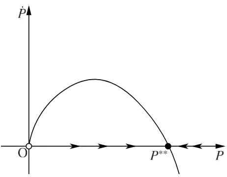
[image:14.595.183.414.432.612.2]Proposition 5. If the Marshall-Lerner condition is satisfied, then the long-run equilibirum is locally stable.
Figure 2 shows the phase diagram for the long run.
P
O
P P
Figure 2: Phase diagram of the terms of trade in the long run
Results of comparative static analysis of the long-run equilibirum are as follows.9)
First, the effects of an increase in the profit share of the North on the capacity utilization rate, the growth rate of the North, the terms of trade, and the growth rate of the South are given by
πN ↑=⇒u∗∗N ↓, g ∗∗
N ↑or↓, P ∗∗ ↑
or↓, g∗∗S ↑or↓ (49)
Since Thirlwall’s law holds in the long-run equilibirum, an increase in the profit share of the North has a similar effect on the growth rates of both countries.
Second, the effects of an increase in the profit share of the South on the capacity utiliza-tion rate, the growth rate of the North, the terms of trade, and the growth rate of the South are given by
πS ↑=⇒u∗∗N−, g ∗∗ N−, P
∗∗ ↓
, g∗∗S − (50)
An increase in the profit share of the South deteriorates the terms of trade but does not affect the growth rate of the South.
Proposition 6. In the long-run equilibirum, an increase in the profit share of the North
either increases or decreases the growth rate of the North. When the growth rate of the North increases, the growth rate of the South increases. In contrast, when the growth rate of the North decreases, the growth rate of the South decreases.
Proposition 7. In the long-run equilibrium, an increase in the profit share of the South does not affect the growth rate of the North and that of the South.
5
Concluding remarks
This study extends the Dutt’s (2002) model that describes uneven development between the North and the South under North-South trade, and investigates changes in income distribu-tions on both countries’ economic growth rates. In our analysis, to capture both a wage-led growth regime and a profit-led growth regime, we use a Marglin-Bhaduri-type investment function instead of a Kalecki-type investment function that is used in Dutt (2002).
income redistribution policy in one country affects the other country’s growth rate through international trade.
Income distributions of the North and the South in our model are exogenously given. However, in reality, income distribution is endogenously determined and affected by the economic growth rate. Therefore, to endogenize income distribution is an important issue and will be left for future research,
Appendix: real wage rate of the North
We investigate the effect of an increase in the profit share of the North on the real wage rate of the North. As in the text, we assume that workers in the North consume both the Northern and the Southern goods. Hence, the real wage rate that workers in the North face
VN is assumed to be given by
VN =
WN
Pα SP
1−α N
= 1
Pα(1+z)b N
= 1−πN
Pαb N
. (51)
The short-run equilibrium value of the real wage rate of the North is given by
VN∗ = 1−πN
bN [
α0(1−sNπN)
β0πεS
S
(u∗NKN)εN (
KS
aS
)−εS]−µN+µαS−1
. (52)
To investigate the effect of an increase in the profit share of the North on the real wage rate of the North, we take the logarithm ofVN∗ as follows:
logVN∗ = log(1−πN)−
α0(u∗NKN)εN−1(P∗)1−µN
µN+µs−1
[log(1−sNπN)+εNlogu∗N]+· · · . (53)
Since∂VN∗/∂πN =VN∗∂logV ∗
N/∂πN, we examin the sign of∂logVN∗/∂πN. Ifαis constant,
then we obtain
∂logVN∗
∂πN
= − 1
1−πN
+ α
µN +µS −1 (
sN
1−sNπN
− εNγ2
γ0+γ2πN
+ εNsN
sNπN−γ1
)
⋛ 0. (54)
Therefore, an increase in the profit share of the North either increases or decreases the real wage rate of the North in the short-run equilibirum. Actually, let πN = 0.3, α = 0.5,
because a slight increase inπN increasesg∗N. We obtain∂logVN∗/∂πN = −0.72 < 0. On the
other hand, let γ1 = 0.09 and γ2 = 0.04 keeping other parameters same. Then, we obtain
u∗
N = 0.87 andg ∗
N = 0.13. In this case, the economy exhibits a wage-led growth because a
slight increase inπN decreasesg∗N. We obtain∂logVN∗/∂πN = 1.51> 0.
We can easily know that an increase in the profit share of the South increases the real wage rate of the North in the short-run equilibrium.
Proposition 8. Suppose that both countries are located in the short-run equilibrium. Then, an increase in the profit share of the North either increases or decreases the real wage rate of the North. On the other hand, An increase in the profit share of the South increases the real wage rate of the North.
The long-run equilibrium value of the real wage rate of the North is given by
VN∗∗ = 1−πN
bN (
εN
εS · aS
sSπS ·g∗∗N
)−αξ
. (55)
To investigate the effect of an increase in the profit share of the North on the real wage rate of the North, we take the logarithm ofV∗∗
N as follows:
logVN∗∗ =log(1−πN)−
α0(u∗∗NKN)εN−1(P∗∗)1−µN
ξ logg
∗∗
N +· · · . (56)
Capital stock of the North KN continues to increase at the rate of g∗∗N > 0 at the long-run
equilibrium. WithεN < 1, the termKεN −1
N approaches zero. Accordingly, the second term of
the right-hand side approaches zero. In this case, we obtain
∂logV∗∗ N
∂πN
= − 1
1−πN
<0. (57)
Therefore, an increase in the profit share of the North decreases the real wage rate of the North in the long-run equilibrium.
We can easily know that an increase in the profit share of the South increases the real wage rate of the North in the long-run equilibrium.
References
Blecker, R. A. (1996) “The New Economic Integration: Structuralist Models of North-South Trade and Investment Liberalization,”Structural Change and Economic Dynamics7, pp. 321–345.
Blecker, R. A. (1998) “International Competitiveness, Relative Wages, and the Balance-of-Payments Constraint,”Journal of Post Keynesian Economics20 (4), pp. 495–526.
Dutt, A. K. (1996) “Southern Primary Exports, Technological Change and Uneven Devel-opment,”Cambridge Journal of Economics20, pp. 73–89.
Dutt, A. K. (2002) “Thirlwall’s Law and Uneven Development,”Journal of Post Keynesian Economics24 (3), pp. 367–390.
Findlay, R. (1980) “The Terms of Trade and Equilibrium Growth in the World Economy,”
American Economic Review70 (3), pp. 291–299.
Marglin, S. and Bhaduri, A. (1990) “Profit-Squeeze and Keynesian Theory,” in S. Marglin and J. Schor (eds.) The Golden Age of Capitalism: Reinterpreting the Postwar Expe-rience, Oxford, Clarendon Press.
McCombie, J. S. L. and Thirlwall, A. P. (1994)Economic Growth and the Balance of Pay-ments Constraint, London: Palgrave Macmillan.
Nakatani, T. (2012) “Significance of Post-Keynesian Economics: Kalacki-Steindl Propo-sition and its Extensions to Open Wage-Led Economies,” Post Keynesian Review1 (1/2), pp. 17–37.
Pugno, M. (1998) “The Stability of Thirlwall’s Model of Economic Growth and the Balance-of-Payments Constraint,”Journal of Post Keynesian Economics20 (4), pp. 559–581.
Rowthorn, R. E. (1981) “Demand, Real Wages and Economic Growth,”Thames Papers in Political Economy, Autumn, pp. 1–39.
Sasaki, H. (2009) “North-South Ricardian Trade and Growth under the Balance of Payments Constraint,”Journal of Post Keynesian Economics31 (2), pp. 299–324,
Sasaki, H. (2013) “Cyclical Growth in a Goodwin-Kalecki-Marx Model,” Journal of Eco-nomics108 (2), pp. 145–171.
Thirlwall, A. P. (1979) “The Balance of Payments Constraint as an Explanation of Interna-tional Growth Rate Differences,”Banca Nazionale del Lavoro Quarterly Review 32, pp. 45–53.
Thirlwall, A. P. (2012) “Balance of Payments Constrained Growth Models: History and Overview,” in Soukiazis and Cerqueira (2012), pp. 11–49.