A novel algorithm for describing population level
trends in body weight
Azadeh Alimadad1,2*, Carrie Matteson3, Warren L. Hare2,4, Ozge Karanfil5, Diane T. Finegood3 1Faculty of Health Sciences, Simon Fraser University, Burnaby, Canada; *Corresponding Author: [email protected]
2Modeling of Complex Social Systems Program, Simon Fraser University, Burnaby, Canada 3Department of Biomedical Physiology & Kinesiology, Simon Fraser University, Burnaby, Canada
4Mathematics, Irving K. Barber School of Arts and Sciences, University of British Columbia, Okanagan Campus, Kelowna, Canada 5Sloan School of Management, Massachusetts Institute of Technology, Cambridge, USA
Received 1 November 2012; revised 9 December 2012; accepted 24 December 2012
ABSTRACT
Modeling population trends and predicting the impact of interventions to address obesity re- quires algorithms for predicting body weight status in the future. Predictions can be based on statistical consideration of different risk factors, or be an extrapolation of past and current trends. Despite the well known correlation between previous and future weight, individual weight history has not been used to predict future trends. We developed a novel population-level model to examine trends of different classes of body weight considering individual body weight histories from the National Longitudinal Survey of Youth (NLSY79). A subset of data used to as- sess the predictive ability of our proposed model with actual data. Our results confirm the impor- tance of weight history in determining future weight status. Over 80% of individuals in a spe- cific weight category (normal, overweight, obese) will stay in the same weight category after two years (except overweight females). The length of body weight stability was also found to be im- portant. The probability of remaining normal weight increased with longer prior periods of being at a normal weight over 18 years (0.834 to 0.893). We demonstrate that an individual’s most probable weight class in the future is consistent with their maximal historical weight class.
Keywords: Body Weight; Modeling; Obesity
1. INTRODUCTION
Obesity and its associated chronic diseases are the leading causes of preventable death worldwide [1]. The obesity epidemic has grown rapidly over the last few
decades and is associated with a growing morbidity and mortality due to diabetes, cardiovascular disease, and cancer [2,3]. To understand the implications for health care systems and public health programs, policy makers need a means of projecting these rates and their related costs into the future. Modeling provides a means of making these projections, as well as an approach to ex- amining options for slowing or reversing current trends [4,5].
Regression analysis is a common modeling technique that has been used to extrapolate the prevalence of over- weight and obesity into the future. Wang et al. used lin-
ear regression to project the prevalence of overweight and obesity among US adults [6]. Their projection sug- gests that by 2048 all Americans will be overweight or obese. One challenge of this approach, however, is in defining the time interval over which historical weight status can be extrapolated into the future [4]. The chal- lenge is due in part to the dynamics of environmental factors like the availability and affordability of food, marketing, accessibility of public transport, and the structure and influence of social networks. In addition, interventions introduced to address overweight and obe- sity may influence trends into the future [7].
Markov modeling is another approach that has been suggested for predicting trends related to obesity and diabetes [5,8-10]. Markov models would consider indi- viduals as belonging to groups based on a parameter like body mass index (e.g. normal weight, overweight or obese) and population trends are determined by the probability of transitioning from one group to another. Simple Markov models require the Markov assumption, that the transition from one state to another is only de- pendent on the current state and not any previous states. However, it is well known that weight status is correlated to prior weight status [11,12], making the Markov as- sumption questionable.
Markov assumption using data from the National Longi- tudinal Survey of Youth (NLSY79). We calculated the transition probabilities between different weight catego- ries over an 18 year period. Our analysis shows that tran- sition probabilities between BMI categories are not solely dependent on an individual’s current weight status. In addition, we introduce a new approach, the Maxhist model, which extends the basic Markov model by in- cluding conditional probabilities, where the probability of being in a specific weight category depends on the highest historical body weight.
2. METHODS AND PROCEDURE
2.1. Description of Data
The National Longitudinal Survey of Youth (NLSY79) dataset is a nationally representative sample of 12,686 young men and women born in the late 1950s and early 1960s in the United States. These individuals were inter- viewed annually from 1979 to 1994 and then biennially from 1994 to 2006. Each individual reported his or her weight at each time point and their height in 1981, 1982 and again in 1985. Body Mass Index (BMI = Weight/ (Height)2 = kg/m2) was calculated using the reported weights and the highest reported height for each individ- ual. We calculated the BMI biennially between the years 1986 and 2004, for all individuals who were 21 years or older in 1986. We excluded 491 subjects for a missing date of birth, 1 subject was excluded for missing height, and 200 subjects we excluded due to pregnancy. Since only 5 individuals were born in 1955, 1956 and 1965, we excluded them as well. The remaining number of sub- jects in this dataset was 11,989. Two subsets of the data were used for this study.
Subset 1: This set of the data was used to calculate transition probabilities between 2 time steps and to ex- plore the effect of an individual’s historical BMI in driv- ing their future BMI using the Markov and Maxhist models. We were interested in how individuals transi- tioned between different classes of BMI. As such we excluded subjects who did not have any consecutive re- ported weights (n = 1261). The remaining sample had 10,728 individuals (50% female). It was used to explore the effect of an individual’s historical BMI in driving their future BMI.
Subset 2: This subset was used to test the accuracy of our Maxhist hypothesis regarding probabilities of par- ticular patterns of population weight transition over time. To verify the accuracy of the Maxhist hypothesis, we used a dataset in which each individual’s BMI was known at every time point. Therefore we excluded indi- viduals if their weight data was missing at any time step. This reduced our sample size to 5316 individuals (49% female). To ensure that this smaller sample is an accurate
representation of the larger population, transition prob- abilities were also calculated on subset 1 using the Max- hist algorithm. Estimated values for transition probabili- ties were similar in both the larger and the reduced data- set.
2.2. Definition of Weight Classes and Age Groups
In order to calculate transition probabilities from one BMI category to another we defined three classes of body weight: NO: Normal weight (BMI < 25), OW: Over- weight (25 ≤ BMI < 30), and OB: Obese (BMI ≥ 30) [5]. The dynamics of weight gain and weight loss in the NLSY79 dataset was investigated with longitudinal data that spanned the interval from 22 to 48 years of age for people born between 1957 and 1964. All subjects of the same age were grouped together regardless of their date of birth due to the small range of years in which subjects were enrolled in the study. Therefore, our group of 24 year olds would consist of individuals who were born in 1962 and were 24 in 1986, plus those individuals who were born in 1964 and were 24 in 1988, etc. We verified that there was no birth cohort effect by comparing the BMI trend lines for each birth cohort.
2.3. Design of the Markov Model
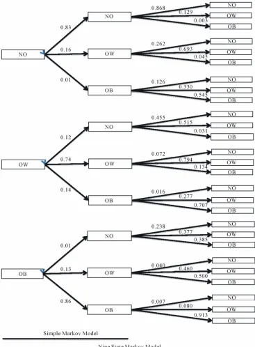
To explore the trends in obesity at the population level, we considered a simple Markov model with 3 states: Normal weight (NO), Overweight (OW), and Obese (OB). We calculated the probability of individuals’ movements between these three states (transition prob- abilities) as follows. At each time interval, individuals are assigned to a state and the probability of staying in that state or moving to one of the other 2 states is calcu- lated for each class from the data in subset 1 (Figure 1, Simple Markov Model, left hand side of the figure). Calculations reflect only the current state of the system and not prior time points. In essence the calculation is “memory-less” and follows the Markov assumption. Since the NLSY79 dataset was collected every two years, we use this time interval as our natural time step (known as Markov cycle) between transitions. As time steps rep-resent two year, we assume that any state can transition into any other state between each time step.
Figure 1. The simple and nine BMI state Markov model.
premise of the “memoryless” property of the Markov model.
2.4. Development of the Maxhist Model
To address the failure of the simple and the 9 state Markov models, we developed a new method for defin- ing the state space by extending our basic model to in- clude a conditional probability. The Maxhist model is based on the premise that an individual’s most probable
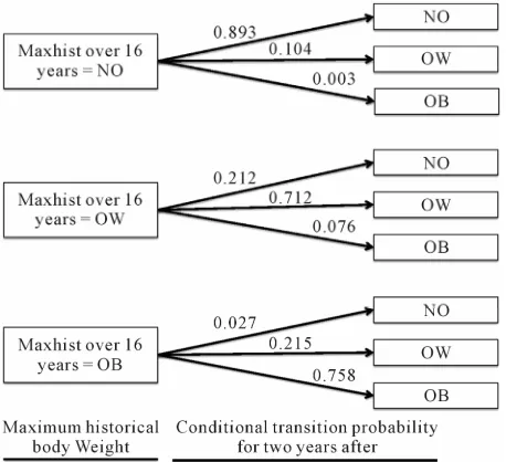
weight class in the future is determined by their maximal historical weight class. The Maxhist function considers an individual’s BMI history for n time steps and returns the maximal historical BMI. We calculate the conditional probability of individual’s movements based on the re- sult of Maxhist function (Figure 2).
2.5. Validation of the Maxhist Algorithm
Figure 2. Illustration of Maxhist model (considering last 16
years of individual’s BMI history to predict their body weight status two years after).
Maxhist algorithm. In the first approach, we determined the number of times the Maxhist hypothesis was broken. This equals the frequency of cases where OW indi- viduals go on to become NO even though their maximum historical body weight was OW and the number of times OB people go on to become NO or OW even though their maximum historical weight was OB.
In order to assess the predictive validity of the pro- posed Maxhist model, we applied a split-sample valida- tion method by separating the dataset into two parts: the first 10 years and the next 8 years of data on each subject. The first part of the dataset was used to calculate transi- tion probabilities, which were then applied to the subse- quent eight years to predict the outcomes. The predic- tions of the Maxhist model were calculated using MATLAB (version 7.5.0.338-R2007b). Values were compared to the results of a simple Markov model and a linear extrapolation based on the first 10 years of data. All three results were compared to the actual body weight classifications in the second half of the dataset. To measure the goodness of fit between the actual and predicted percentage of NO, OW and OB, the square root of the sum of the square differences are calculated be- tween the age of 34 and 40 (see Equation (1) below).
3. RESULTS
3.1. Markov Transition Probabilities
The probabilities that an individual in each BMI cate-
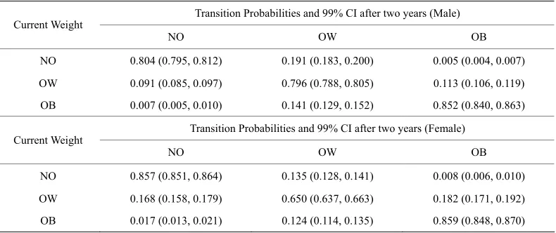
gory (NO, OW, OB) moves to any of these three states after two years (one time step) for males and females in the NLSY79 data subset #1 are shown in Table 1.
For example, men who are OB have a 14.1% chance of becoming OW in the subsequent two years. The probability that individuals could have an extreme weight change over two years (e.g. NO to OB) is very rare in both male and female groups (0.5% and 0.8% respectively). Likewise the transition from OB to NO is rare but slightly higher for women as compared to men (M: 0.7% and F: 1.7% respectively).
The results demonstrate that there is an over 80% chance that a male in the NO weight category will stay in the same weight category, and an almost 80% chance that an OW male will stay in the OW category in the next two-years. This probability is even higher for the OB, as we find that 85% of individuals are likely to re- main OB after two years. Women in the NO and OB categories behave similarly to men, but the transition probability for an overweight woman to remain OW is only 65%, whereas it is almost 80% for men. Thus, there is an almost 15% difference between males and females in this category, which suggests that women are more susceptible to weight fluctuations than men, and in both directions.
The above results are based on two years weight tran- sitions, which shows the current weight of individuals can play an important role in driving their future weight status. If an individual’s future body weight depends only on their current body weight and is independent of their previous body weight, we could use a simple Markov model to project individual’s body weight over time.
3.2. Evaluating the Markov Assumption
For the basic Markovian principles to hold true, we would have to see that an individual’s previous body weight would have no impact on their future weight. Consider for example the following 3 transitions: 1) NO → NO → NO; 2) OW → NO → NO; 3) OB → NO → NO. If prior weight has no effect on future weight then the second transition from NO → NO should have the same transition probability in all three cases. Figure 1 illustrates that these probabilities and their 95% confi- dence intervals are 0.868 (0.863, 0.874), 0.455 (0.428, 0.481) and 0.238 (0.138, 0.337) respectively. Hence, the Markov assumption does not hold. Likewise the Markov assumption does not hold for the transition from OB → OB where an OB prior state increases the probably of remaining OB (0.913 (0.905, 0.921)) as compared to an
2
2age34 age34 age40 age40
[image:4.595.58.287.85.294.2]Table 1. Transition Probabilities for each BMI state independent of age (row to column).
Transition Probabilities and 99% CI after two years (Male) Current Weight
NO OW OB
NO 0.804 (0.795, 0.812) 0.191 (0.183, 0.200) 0.005 (0.004, 0.007)
OW 0.091 (0.085, 0.097) 0.796 (0.788, 0.805) 0.113 (0.106, 0.119)
OB 0.007 (0.005, 0.010) 0.141 (0.129, 0.152) 0.852 (0.840, 0.863)
Transition Probabilities and 99% CI after two years (Female) Current Weight
NO OW OB
NO 0.857 (0.851, 0.864) 0.135 (0.128, 0.141) 0.008 (0.006, 0.010)
OW 0.168 (0.158, 0.179) 0.650 (0.637, 0.663) 0.182 (0.171, 0.192)
OB 0.017 (0.013, 0.021) 0.124 (0.114, 0.135) 0.859 (0.848, 0.870)
Data for transition probabilities are presented with 99% confidence intervals in the parenthesis.
NO or OW prior state (0.545 (0.452, 0.637) and 0.707 (0.684, 0.730), respectively).
3.3. Maxhist Model
Given the importance of prior body weight, we exam- ined a new model (Maxhist) which calculates transition probabilities for a future transition based on the maxi- mum historical body weight. Transition probabilities were calculated for each possible subset of historical data,
i.e. for prior knowledge of 2, 4, 6, etc. or up to 16 prior
years of information (at 2 year intervals). Table 2 pro- vides the results for the maximum historical period available (16 years) in the NLSY79 dataset (other data not shown). This table demonstrates that the highest probabilities are for transitions that are determined by the highest historical body weight, e.g. Maxhist (NO) → NO is 0.892, Maxhist (OW) → OW is 0.712 and Maxhist (OB) → OB is 0.758.
Not surprisingly, the length of historical body weight maintenance in a single category increases the probabil- ity of remaining in that category as illustrated in Table 3. The probability of remaining in NO increased with longer prior periods of being NO (from 0.834 to 0.893), and the probability of transitioning to OW decreases slightly with longer periods of NO weight maintenance (from 0.159 to 0.104). The probability of transitioning to OB from NO is low regardless of the length of time be- ing NO prior to the transition (less than 1%).
To check the robustness of these results, we repeated this analysis with the smaller dataset #2 (individuals with weight recorded at every time step) and also repeated this experiment working by years instead of age and found essentially the same results (data not shown).
3.4. Evaluating the Maxhist Assumption
According to the Maxhist hypothesis, individuals have
a strong tendency to return to their highest historical BMI status at the population level, however, there are individuals who don’t necessarily return to their highest historical weight. This is reflected for example in the fact that even individuals with a Maxhist of OW have a 21.2% chance of becoming NO (Table 2). This would reflect a “break” from the Maxhist hypothesis. An individual who was OB or OW once and then maintained a reduced body weight (e.g. they were OB → NO → NO → NO → NO → NO → NO) would repeatedly break the Maxhist hypothesis because they never returned to their highest historical body weight.
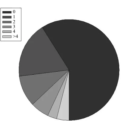
To explore the transitions of the BMI status at the individual level, we used subset #2 (individuals with weight recorded at every time step) who had 18 years of data. For each individual, we counted the number of times when BMI was lower than the maximum historical weight. Well over half of the subjects in this dataset never broke the Maxhist hypothesis and more than 25% break it only once or twice, while a small percentage of all people break the Maxhist hypothesis more than 3 times within an 18-year interval (Figure 3).
3.5. Model Simulation, Validation and Predictions
Table 2. Probability of being in NO, OW, or OB given maximum historical BMI in the last 16 years is NO,
OW, or OB.
Probability of being in specific BMI 2 years after Maximum historical BMI
within the last 16 years NO OW OB
NO 0.893 (0.882, 0.905) 0.104 (0.093, 0.115) 0.003 (0.001, 0.004)
OW 0.212 (0.200, 0.225) 0.712 (0.0698, 0.726) 0.076 (0.068, 0.084)
OB 0.027 (0.022, 0.033) 0.215 (0.201, 0.228) 0.758 (0.744, 0.772)
[image:6.595.97.497.239.410.2]*Data for transition probabilities are presented with 99% confidence intervals in the parenthesis.
Table 3. Probability of being in state NO, OW, or OB given that the maximal historical BMI state is NO.
Time step P (NO) given Maxhist = NO P (OW) given Maxhist = NO P (OB) given Maxhist = NO
2 0.834 (0.829, 0.839) 0.159 (0.154, 0.164) 0.007 (0.006, 0.008)
4 0.860 (0.855, 0.865) 0.135 (0.130, 0.140) 0.004 (0.003, 0.005)
6 0.870 (0.864, 0.875) 0.127 (0.121, 0.132) 0.004 (0.003, 0.005)
8 0.876 (0.870, 0.822) 0.121 (0.115, 0.126) 0.003 (0.002, 0.004)
10 0.882 (0.876, 0.888) 0.115 (0.109, 0.121) 0.003 (0.002, 0.004)
12 0.886 (0.878, 0.893) 0.111 (0.104, 0.118) 0.003 (0.002, 0.005)
14 0.889 (0.881, 0.897) 0.108 (0.100, 0.116) 0.003 (0.002, 0.005)
16 0.892 (0.882, 0.901) 0.106 (0.096, 0.115) 0.003 (0.001, 0.004)
18 0.893 (0.882, 0.905) 0.104 (0.093, 0.115) 0.003 (0.001, 0.004)
*Data for transition probabilities are presented with 99% confidence intervals in the parenthesis.
0 1 2 3 4 >4
[image:6.595.73.274.423.624.2]Number of times the Maxhist hypothesis is broken
Figure 3. Illustration of the strength of Maxhist
hy-pothesis.
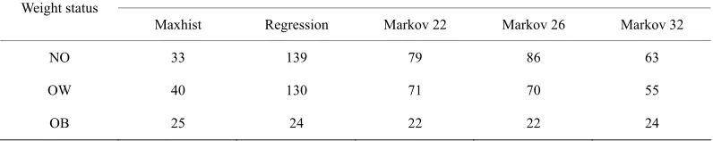
see that the Maxhist model provides a significantly better fit to the actual data than the linear regression, and also better than the three state Markov model. Table 4 pre- sents the sums-of-squares results for each of the models tested for NO, OW and OB.
Age (years)
22 26 30 34 38 42 46
P
ercentage of
NO
-20 0 20 40 60
[image:6.595.310.537.435.614.2]Actual Maxhist Regression Markov
Figure 4. Model simulation results.
Examining Table 4 it is clear that the Maxhist model makes significantly better predictions for the proportion of NO and OW than any other model. The model accu- racy for OB is similar to all approaches.
4. DISCUSSION
Table 4. Sum-of-squares difference between the percentage of people predicted and actual in each weight
category.
Sum-of-squares difference between the actual weight and predicted values Weight status
Maxhist Regression Markov 22 Markov 26 Markov 32
NO 33 139 79 86 63
OW 40 130 71 70 55
OB 25 24 22 22 24
strated that prior body weight of individuals can play an important role in defining an individual’s future weight [11-13]. Using longitudinal cohorts, Miller et al. [11] and
Stark et al. [12] demonstrated the risk of being over-
weight in adulthood is greater for overweight children compare to those who were normal weight as children. Abraham and Nordsieck also showed overweight chil- dren (age 10 - 13) are about twice as likely to become overweight adults 20 years later as compared to children with average weight [13]. Consistent with these observa- tions, our study shows that overweight and obese young adults are likely to remain overweight or obese over the next 18 years. In addition, we show that the probability of remaining NO increased with longer prior periods of being NO and individuals who become OW and OB are not likely to return to a lower body weight over time.
This modeling approach helps visualize the need for stronger emphasis on preventive measures and making concerted efforts to curb childhood obesity as early as possible to avoid lengthy time intervals where increased weight status becomes a powerful predictor of continued weight management challenges.
Although the relationship between early body weight and body weight in adulthood was well known, current modeling approaches for projecting future trends in obe- sity have not taken this relationship into account. Current methods for projecting trends in obesity have used linear extrapolations based on the prevalence of obesity over time. As such these models do not take into account in- dividual weight status. Some authors have suggested that Markov models could be used to consider individual weight status, but we demonstrate that a simple Markov model is not adequate and there is insufficient data available on which to base higher order Markov models.
We developed a novel model (Maxhist) by considering the importance of an individual’s weight history. Our algorithm uses conditional probabilities, where the like- lihood of being in a specific weight category depends on the highest historical body weight. The main advantage of the Maxhist model is that it takes into account the weight history of individuals with a minimum amount of data. In theory we could use a higher order Markov model (e.g. 9 state model) but this requires a very large
dataset for the calculation of all of the relevant transition probabilities.
We compared the capability of the Maxhist model to predict future weight status to a simple 3 state Markov model and a regression model. Our results demonstrate that Maxhist is more accurate than both the Markov and regression models for predictions over a period of 6 years. In addition, the Maxhist model produced more plausible predictions further into the future. It should be noted however, that there was no significant difference in the projections specifically for OB subjects between Maxhist and Markov or Maxhist and regression model.
Not all individuals followed the Maxhist algorithm perfectly during the 18 years of follow up. When indi- viduals move from a higher weight category to a lower weight category they are considered to break the Maxhist hypothesis. However, few people break the Maxhist hy- pothesis (by maintaining a lower weight than the previ- ous time step) more than twice during the 18 year fol- low-up period. Most of the breaks in the Maxhist hy- pothesis are due to OB individuals becoming OW or OW individuals becoming NO. Women are more likely to break the Maxhist hypothesis than men, indicating a grater propensity for weight fluctuations in females.
Our results are based on the analysis of individuals between 22 and 46 years of age who lived in United States. Future studies need to examine generalizability of our algorithm considering different age categories, social, cultural, environmental and demographic factors. There was no birth cohort effect within our study, although this may be due to the small range of birth dates (1957-1964) of individuals in the dataset.
lation prevalence data.
5. ACKNOWLEDGEMENTS
This work is the result of an interdisciplinary collaboration. We thank Dr. Krisztina Vasarhelyi and Dr. Alexander Rutherford for hav- ing enabled this connection across departments. We are indebted to Dr. Nate Osgood for his feedback on the analysis. This work was spon- sored by grants from the Canadian Institutes of Health Research to Dr. Diane T. Finegood and was supported in part by the SFU CTEF MoCSSy Program. We also are grateful for technical support from the IRMACS Centre, Simon Fraser University. Parts of this study were presented in preliminary form as an abstract at the First Annual Work- shop on Dynamic Modelling for Health Policy.
REFERENCES
[1] Mokdad, A.H., Marks, J.S., Stroup, D.F. and Gerberding J.L. (2004) Actual causes of death in the United States, 2000. American Medical Association, 291, 1238-1245.
[2] Flegal, K.M., Carroll, M.D., Ogden, C.L. and Johnson C.L. (2002) Prevalence and trends in obesity among US adults, 1999-2000. American Medical Association, 288,
1723-1727.
[3] Wang, Y. and Lobstein, T. (2006) Worldwide trends in childhood overweight and obesity. International Journal of Pediatric Obesity, 1, 11-25.
doi:10.1080/17477160600586747
[4] Basu, A. (2010) Forecasting distribution of body mass index in the United States: Is there more room for growth? Medical Decision Making, 30, E1-E11.
doi:10.1177/0272989X09351749
[5] Huang, E.S. and Basu, A. (2009) Projecting the future diabetes population size and related costs for the US. Diabetes Care, 32, 2225-2229.
doi:10.2337/dc09-0459
[6] Wang, Y., Beydoun, M.A., Liang, L., Caballero, B. and Kumanyika, S.K. (2008) Will all Americans become overweight or obese? Estimating the progression and cost of the US obesity Epidemic. Obesity, 16, 2323-2330. doi:10.1038/oby.2008.351
[7] Brown, M., Byatt, T., Marsh, T. and McPherson, K. (2009) Obesity trends for children aged 2 - 11, analysis from the health survey for England 1993-2007. Report by the Na-tional Heart Forum.
[8] Huang, E.S., Basu, A., O’Grady, M.J. and Capretta, J.C. (2009) Using clinical information to project federal health care spending. Health Affairs, 28, w978-w990.
doi:10.1377/hlthaff.28.5.w978
[9] Ortegon, M.M., Redekop, W.K. and Niessen, L.W. (2004) Cost effectiveness of prevention and treatment of the diabetic foot. Diabetes Care, 27, 901-907.
doi:10.2337/diacare.27.4.901
[10] Van Baal, P.H.M., Polder, J.J., De Wit, G.A., Hoogenveen, R.T., Feenstra, T.L., Boshuizen, H.C., Engelfriet, P.M. and Brouwer, W.B.F. (2008) Lifetime medical costs of obesity: Prevention no cure for increasing health expen- diture. PLoS Medicine, 5, e29.
doi:10.1371/journal.pmed.0050029
[11] Miller, F.J.W., Billewicz, W.Z. and Thomson, A.M. (1972) Growth from birth to adult life of 442 Newcastle upon Tyne children. British Journal of Prevention and Social Medicine, 26, 224-230
[12] Stark, O., Atkins, E., Wolff, O.H. and Douglas, J.W.B. (1981) Longitudinal study of obesity in the National Sur-vey of Health and Development. British Medical Journal,
283, 13-17. doi:10.1136/bmj.283.6283.13