LnCm fault model : complexity and validation

(1)

warwick.ac.uk/lib-publications

A Thesis Submitted for the Degree of PhD at the University of Warwick

Permanent WRAP URL:

http://wrap.warwick.ac.uk/92013

Copyright and reuse:

This thesis is made available online and is protected by original copyright.

Please scroll down to view the document itself.

Please refer to the repository record for this item for information to help you to cite it.

Our policy information is available from the repository home page.

(2)

M A E

G NS

I T A T MOLEM

U N

IV ER

SITAS WARWICEN SIS

L

n

C

m

Fault Model: Complexity and Validation

by

Fatimah Adamu-Fika

A thesis submitted to The University of Warwick

in partial fulfilment of the requirements

for admission to the degree of

Doctor of Philosophy

Department of Computer Science

The University of Warwick

(3)

Abstract

Computer systems are ubiquitous in most aspects of our daily lives, as such the

reliance of end users upon their correct and timely functioning is on the rise.

With technology advancement, the functionality of these systems is increasingly

being defined in software. On the other hand, feature sizes have drastically

de-creased, while feature density has increased. These hardware trends will keep

happening as technology continues to advance. Consequently, power supply

voltage is ever-decreasing and clock frequency and temperature hotspots are

increasing. This steady reduction of integration scales is increasing the

sensi-tivity of computer systems to different kinds of hardware faults. In particular,

the likelihood of a single high-energy ion to cause double bit upsets (DBUs,

due to its energy) or multiple bit upsets (MBUs, due to the incident angle)

in-stead of single bits upsets (SBUs) is increasing. Furthermore, the likelihood of

perturbations occurring in the logic circuits is also increasing. Owing to these

hardware trends it has been projected that computer systems will expose such

hardware faults to the software-level and accordingly the software is expected

to tolerate such perturbations to maintain correct operations, i.e., the software

needs to be dependable. Thus, defining and understanding the potential impact

of such faults is required to propose the right mechanisms to tolerate their

oc-currence. To ascertain that software is dependable, it is important to validate

the software system. This is achieved through the emulation of the type of

faults that are likely to occur in the field during execution of the system, and

through studying the effects of these faults on the system. Often, this validation

process is achieved through a technique called fault injection, that artificially

perturbs the execution of the system through the emulation of hardware faults.

(4)

Traditionally, the single bit-flip (SBF) model is used for emulating single event

upsets (SEUs) and single event transients (SETs) in dependability validation.

The model assumes that only an SEU or SET occurs during a single execution

of the system. However, with MBUs becoming more prominent, the accuracy of

the SBF model is limited. Hence, the need for including MBUs in software

sys-tem dependability validation. MBUs may occur as multiple bit errors (MBEs)

is a single location (memory word or register) or as single bits errors (SBEs) in

several locations. Likewise, they may occur as MBEs in several locations.

In the context of software-implemented fault injection (SWIFI), the injection of

MBUs in all variables is infeasible due to the exponential size of the fault space,

thereby making it necessary to carefully select those fault injection points that

maximises the probability of causing a failure. A fault space, is the set of all

possible fault under a given fault model. Consequently, research have started

looking at a more tractable model, double bit upsets (DBU) in the form of

double bit-flips within a single location, L1C2. However, with evidence of the

possibility of corruption occurring chip wide, the applicability and accuracy of

L1C2 is restricted. Following, this research focuses on MBUs occurring across

multiple locations whilst seeking to address the exponential fault space problem

associated with multiple fault injections.

In general, the thesis analyses the complexity of selecting efficient fault-injection

locations1_{for injecting multiple MBUs. In particular, it formalises the problem}

of multiple bit-flip injections and found that the problem is NP-complete. There

are various ways of addressing this complexity: (i) look for specific cases, (ii)

look for heuristic and/or (iii) weaken the problem specification.

Next, the thesis presents one approach for each of the aforementioned means of

addressing complexity:

• for the specific cases approach, the thesis presents a novel DBU fault

1_{injection points that would uncover vulnerabilities and/or cause system failure.}

(5)

model, that manifest as two single bit-flips across two locations. In

par-ticular, the research examines the relevance of the L2C1 fault model for

system validation. It is found that the L2C1 fault model induces failure

profile that is different from profiles induced by existing fault models.

• for the heuristic approach, the thesis uses an approach towards

depen-dency aware fault injection strategies to extend the L2C1fault model and

the existing L1C2 fault model into LnCm(multiple location, multiple

cor-ruption) fault model, wheren is the number of locations to target and

m the maximum number of corruptions to inject in a given location. It

proposes two heuristics to achieve this: first, select the set of potential

locations and then select the subset of variables within these locations,

and it examines the applicability of the proposed framework.

• for the weakening of the problem specification approach, the thesis further

refines the fault space and proposes a data mining approach to reduce the

cost of multiple fault injections campaigns (in terms of number of multiple

fault injections experiments performed). It presents an approach to refine

the multiple fault injection points by identifying a subset of these points,

whereby injection into this subset alone would be as efficient as injection

into the entire set.

These contributions are instrumental to advance multiple fault injections and

make it an effective and practical approach for software system validation.

(6)

To my Mamah and Baba,

For their endless love, support and encouragement.

Also to the memory of

my dear Iya, Khadijah Tasalla Fika,

my favourite uncles, Emir Abali Ibn Muhamad

& Mallam Jibril Amfani,

my darling aunt, Zainabu “Ya Abu” Amfani,

and

my dear cousins, Bilkisu Fika,

(7)

Acknowledgements

First and foremost, I give my utmost gratitude to God for letting me reach this

point of my graduate education.

I am forever indebted to Islamic Development Bank for granting me a

scholar-ship to undertake my graduate studies, and also to Yobe State government for

their financial aid. Without these grants it wouldn’t have been possible to be

writing this thesis now.

Throughout my graduate education Dr. Arshad Jhumka has been an excellent

supervisor, mentor and most of all friend. He saw what I did not see in myself

and pushed me hard to achieve what he knew I could. I doubt very much I

would gotten to this stage with out his guidance and support. I would also like

to thank my former supervisor, Sarab Singh, for accepting me as a student, and

for being a friend and mentor.

I am especially thankful to my mentors Dr. Ardo Bamanga, Mr. Musa Maina

Mshelia and Mr. Lekan Muyiwa Ogedengbe, for their unwavering support and

advise. I thank you all from the bottom of my heart. My sincerest gratitude to

keen sounding boards Hadiza Fika, Hadi Fika and Hassana Fika-Mohammed,

for always having time for (and never getting irritated by) my constant whining

and nagging.

I would also like to express my gratitude to my colleagues who turned friends,

who motivated me through out my graduate journey - especially, Saima Arif,

Nentawe Gurumdimma, Adekunle Shonola, Daniel Onah and Daniel Nwaigwe.

I am also thankful to the entire staff of the Computer Science Department,

(8)

especially the members of the Systems and Software group.

To my friends, old and new - most especially, Maryam Uwani Abdullahi, Safiya

& Sharif Abdullahi, Nana & Jonathan Lyamgohn, Asmau “Aims” Smaila, Sani

Sidi, Alheri Loma, Fatima Goje, Ibrahim Muazzam, Abdul Isa Waziri, Jamilla

Bello and my LIS ’95 and Gwags tribes - I say a big thank you! You all helped

my sanity remain sane through this arduous journey.

Not least of all, I owe so much to my whole family and family friends for their

undying support, their unwavering belief that I can achieve so much.

Unfortu-nately, I cannot thank everyone by name because it would take a lifetime but, I

just want you all to know that you count so much. Had it not been for all your

prayers and benedictions; were it not for your sincere love and help, I would

never have completed this thesis. So thank you all.

(9)

Declarations

This thesis include and extends materials from the following works:

[2] F. Adamu-Fika and A. Jhumka. An investigation of the impact of

dou-ble single bit-flip errors on program executions. In P. Lorenz and F. P.

Dini, editors,DEPEND 2015, The Eight International Conference on

De-pendability, pages 15 – 22, Venice, Italy, August 2015. IARIA. ISBN

978-1-61208-429-9. URLhttp://www.thinkmind.org/index.php?view=

article&articleid=depend_2015_1_40_50038

[1] F. Adamu-Fika and A. Jhumka. Algorithms and Architectures for

Par-allel Processing: 15th International Conference, ICA3PP 2015,

Zhangji-ajie, China, November 18-20, 2015, Proceedings, Part IV, chapter An

Investigation of the Impact of Double Bit-Flip Error Variants on

Pro-gram Execution, pages 799–813. Springer International Publishing, Cham,

2015. ISBN 978-3-319-27140-8. doi: 10.1007/978-3-319-27140-8 55. URL

http://dx.doi.org/10.1007/978-3-319-27140-8_55

(10)

Sponsorship and Grants

The research presented in this thesis was made possible by the support of the

following benefactors and sources:

• Islamic Development Bank:

Merit Scholarship Programme for High Technology (MSP)

(2011–2014)

• Yobe State, Nigeria:

PhD Scholarship Grant

(2014–2015)

(11)

Abbreviations

ARFF Attribute-Relation File Format

ALU Arithmetic Logic Unit

AUC Area Under ROC Curve

CFG Control Flow Graph

COTS Commercial-Off-The-Shelf

CPU Central Processing Unit

DBU Double Bit Upsets

DF Dominance Frontier

DRAM Dynamic Random Access Memory

EXP Exponential Time

FI Fault Injection

FIT Failures-In-Time

FN False Negative

FNR False Negative Rate

FP False Positive

FPR False Positive Rate

IC Intergrated Circuit

ILS Injection Location Selection

ISA Instruction Set Architecture

LnCm Multiple-Locations Multiple Corruptions

LLFI Low Level FI

LLVM Low Level Virtual Machine

MATLAB MATrix LABoratory

MBF Multiple Bit-Flips

(12)

MBU Multiple Bit Upsets

MDS Minimum Dominating Set

MDT Mean Down Time

MEU Multiple Event Upsets

MET Multiple Event Transients

MRI Magnetic Resonance Imaging

MSB Multiple Single Bit-Flips

MTBF Mean Time Between Failures

MTVS Minimum TVS

MVC Minimum Vertex Cover

NP Non-deterministic Polynomial Time

P Polynomial Time

PGM Portable Gray Map

SER Soft-Error Rate

SEU Single Event Upset

SBF Single Bit-Flip

SBU Single Bit Upset

SD Standard Deviation

SDC Silent Data Corruption

SEU Single Event Upset

SEU Single Event Transient

SFI Software FI

SRAM Static Random Access Memory

SWIFI Software-Implemented FI

SIHFT Software-Implemented Hardware Fault Tolerance

ROC Receiver Operating Characteristic

TN True Negative

TNR True Negative Rate

TP True Positive

(13)

TPR True Positive Rate

TVS Target Variable Set

(14)

List of Figures

2.1 Dependability tree. [7] . . . 9

2.2 An overview of fault and error terminology focused on the tran-sient hardware fault. . . 14

2.3 An overview of the relationshipship of an 8-bit MBU and a 3-bit data word with an 8-bit interleave. . . 15

2.4 Block diagram of propagation of soft-error impacting software. . 15

2.5 Overview of fault tolerance coverage [7]. . . 18

2.6 An overview of a basic fault injection environment. . . 20

2.7 An overview of fault tolerance validation. . . 20

2.8 An overview of dependability analysis. . . 22

3.1 Example of basic blocks for a dummy program and its corre-sponding CFG. . . 24

3.2 LLFI workflow [156]. . . 35

4.1 An overview of the thesis contributions. . . 45

6.1 An overview of double faults. . . 65

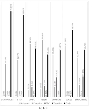
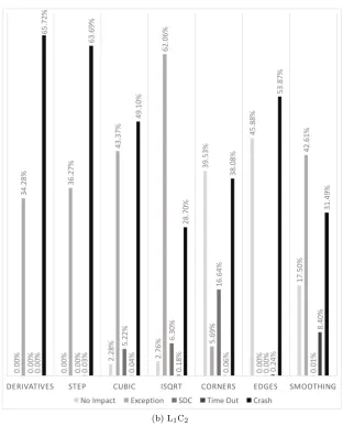
6.2 Error sensitivity distribution of the various fault models for each programs. . . 73

(22)

6.2 Error sensitivity distribution of the various fault models for each

program. . . 74

6.2 Error sensitivity distribution of the various fault models for each

program. . . 75

6.3 Error sensitivity distribution of instruction type for the fault

models over all target programs. . . 86

6.4 Error sensitivity distribution of data type for the fault models

over all target programs. . . 89

7.1 Example of a dominator tree for a CFG and its corresponding

dominance relationships. . . 104

7.2 An overview for the execution of the proposed framework to select

efficient target variables. . . 108

7.3 (Extended) CFG for Isqrt . . . 111

7.4 Dominator tree for Isqrt . . . 113

(23)

7.5 Dependency graph superimposed on dominator tree for Isqrt over

its potential injection location set. . . 114

7.6 Variable Graph for Isqrt . . . 115

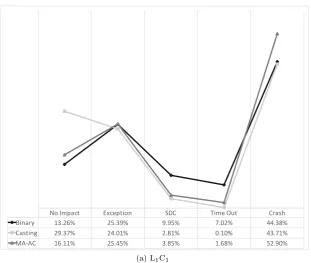
7.7 Average error sensitivity distribution over all target programs for

different variable selection methods. . . 128

8.1 Workflow for generating efficient fault injection points. . . 154

8.2 An overview of generated data set. . . 159

(24)

List of Tables

6.1 Register classificaiton scheme . . . 70

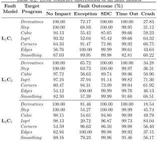
6.2 Error resilience distribution of all fault models . . . 77

6.3 Null hypotheis test results for fault model effect on error resilience 78

6.4 Estimated marginal means for error resilience of all fault models 79

6.5 Pairwise comparisons between mean for all fault models . . . 80

6.6 Confidence interval of error resilience for all blocks . . . 83

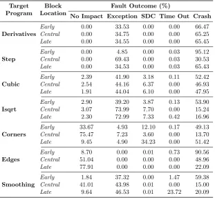
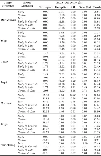
6.7 Error sensitivity distribution for different block locations under

L1C1. . . 83

L1C2. . . 84

L2C1. . . 85

6.10 Spearman’s rank-order correlations . . . 92

6.11 Pearson product moment correlations . . . 93

7.1 Number of target variables selected for the different target programs117

7.2 Total number of fault injection experiments conducted over all

target programs . . . 118

(25)

7.3 Average error sensitivity distributions for different programs for

L1C1 . . . 120

L1C2 . . . 121

L1C3 . . . 122

L1C4 . . . 123

L2C1 . . . 124

L3C1 . . . 125

L4C1 . . . 126

L2C2 . . . 127

8.1 The general form of a confusion matrix for binary classification. 146

8.2 (Double) Injection points efficiencies for na¨ıve Bayes with no

sam-pling . . . 162

8.3 (Triple) Injection points efficiencies for na¨ıve Bayes with no

sam-pling . . . 163

8.4 (Quadruple) Injection points efficiencies for na¨ıve Bayes with no

sampling . . . 164

(26)

8.5 (Double) Injection points efficiencies for rule induction with no

sampling . . . 164

8.6 (Triple) Injection points efficiencies for rule induction with no

sampling . . . 165

8.7 (Quadruple) Injection points efficiencies for rule induction with

no sampling . . . 165

8.8 (Double) Injection points efficiencies for decision tree induction

with no sampling . . . 166

8.9 (Triple) Injection points efficiencies for decision tree induction

with no sampling . . . 167

8.10 (Quadruple) Injection points efficiencies for decision tree

induc-tion with no sampling . . . 167

8.11 (Double) Injection points efficiencies for na¨ıve Bayes with sampling169

8.12 (Triple) Injection points efficiencies for na¨ıve Bayes with sampling 169

8.13 (Quadruple) Injection points efficiencies for na¨ıve Bayes with

sampling . . . 170

8.14 (Double) Injection points efficiencies for rule induction with

sam-pling . . . 170

8.15 (Triple) Injection points efficiencies for rule induction with sampling170

8.16 (Quadruple) Injection points efficiencies for rule induction with

sampling . . . 171

with sampling . . . 171

(27)

8.18 (Triple) Injection points efficiencies for decision tree induction

with sampling . . . 172

8.19 (Quadruple) Injection points efficiencies for decision tree

induc-tion with sampling . . . 172

8.20 (Double) Injection points efficiencies for na¨ıve Bayes with no

sam-pling using full bit set . . . 174

8.21 (Double) Injection points efficiencies for rule induction with no

sampling using full bit set . . . 174

with no sampling using full bit set . . . 174

8.23 (Double) Injection points efficiencies for na¨ıve Bayes with

8.24 (Double) Injection points efficiencies for rule induction with

with sampling using full bit set . . . 176

(28)

List of Algorithms

7.1 Heuristic for Injection Location Selection (ILS) . . . 105

7.2 Heuristic for Target Variables Selection . . . 107

7.3 Algorithm to obtain avariablegraph . . . 116

(29)

CHAPTER

1

Introduction

Modern computer systems are now an inextricable part of the structure of

mod-ern societies. Part of these systems is often a computer control system, a

mi-crocontroller. A microcontroller is usually a self-contained system having a

processor, memory and peripherals and can be used as an embedded system.

Often microcontrollers are embedded in other machinery, such as automobiles,

telephones, appliances, and peripherals for computer systems. Embedded

sys-tems range from portable devices, such as tablets and digital watches, to large

stationary infrastructures, such as traffic lights, industrial process controllers

and largely complex systems like hybrid vehicles, Magnetic Resonance Imaging

(MRI) and avionics. Integral part of virtually all modern computer systems

are integrated circuits (ICs). An IC is an electronic circuits on small plate of

semiconductor device, usually silicon. As technology advances, IC scaling

trans-lates to a shrinkage in the feature size, reduction in supply voltage levels and

increase in feature density and operation frequency. A microprocessor is an IC,

or at most a few ICs, that contains all, or most of, the functions of a central

processing unit (CPU) of a computer; and it is sometimes called a logic chip.

Microprocessors are designed to perform binary, logic and arithmetic, operations

that employs the usage of small number-holding areas called registers. Typical

microprocessor operation include adding, subtracting, comparing two numbers,

and writing and reading numbers to and from one area to another. These

oper-ations are the result of a set of instructions that are part of the microprocessor

design. This set of instructions is called instruction set architecture (ISA), i.e.,

(30)

CHAPTER 1. INTRODUCTION 2

the ISA provides commands to the processor, to tell it what it requires to do.

The ISA consist of different components which include (processor) registers. A

register is one of a small set of data and it may hold an instruction, a storage

address, or any kind of data (e.g., a bit sequence or individual characters). The

low cost of IC made it possible for modern computer systems to pervade our

everyday life. As such, this pervasive nature of these systems has increased our

reliance upon such systems to provide correct and timely service.

However, these current hardware trends has exacerbated the unreliability of

modern computer systems. As technology scales down, their sensitivity to their

environment increases, as a result the probabilities of transient faults and

soft-errors are increasing. A soft-error is an issue that causes a temporary condition

in memory that alters stored data in an unintended way. This means, emerging

technology are error prone to ionising radiation normally caused by low-energy

neutrons coming from cosmic rays and alpha particles coming from packaging

materials. Similarly, soft-error rate (SER) in logic circuits is increasing [111]

and now comparable to the SER in unprotected memory, and the probability

of multiple faults occurring in such devices is equally on the rise. Futhermore,

these emerging technology are projected, in the near-future, to cause computer

systems to expose hardware faults to the information-level, and to ensure that

the software performs as specified [24, 28, 98, 114, 138]. Similarly, it has been

demonstrated that many hardware faults manifest as multiple soft-errors [19].

All of these and the concomitant high cost associated with exclusively tolerating

such faults at the hardware-level necessitate the design of software error resilient

mechanisms and evaluating them under such hardware faults.

The type of fault tolerance to adopt and how to implement it is directly related

and strongly dependent upon the underlying fault assumption. One of the

major issues of designing fault tolerant systems is ensuring such systems meets

their reliability requirements, that is, validating them. This is usually done

(31)

1.1. MOTIVATIONS 3

with [7, 124]. For a large part of applications, especially safety criical system,

it is important to ascertain the coveragw of the fault inection process. There

are other types of application that are not safety critical but may be prone

to dervice degradation as a result of MBU, e.g., an image processing software

rendering a blurry image. This motivates the need of multiple soft-errors model

for designing and evaluating fault tolerant software systems.

1.1 Motivations

Research has shown assumptions about the types of faults that impact a

soft-ware system and how they may affect the system are crucial in the design of a

fault tolerant software system. Thus, dictating the relevant fault tolerance to

implement. Similarly, such assumptions are relevant for the evaluation of the

efficacy of the implemented fault tolerance mechanisms. As such, the emergence

of multiple soft-errors and the eventuality of these errors increasing in the near

future limits the accuracy of the traditional single fault model assumed during

software dependability assessment. Similarly, the manifestation of soft-errors in

several locations, including in logic circuits, constricts the applicability of the

existing double faults model, emulating two soft-errors originating from a single

location, assumed during software system dependability evaluation. Following,

this motivates the need to define a multiple-locations multiple-corruptions fault

model, to emulate multiple soft-errors occurring in several points, during

de-pendable software assessment, which is the focus of the research presented in

this thesis.

However, to assume a multiple-locations multiple-corruptions fault model for

SWIFI three related issues arises; the problem of determining: (i) the injection

location, i.e where to inject, (ii) the injection time, i.e., when to inject, and (iii)

injection latency, i.e., how long to inject. The focus of the research presented

(32)

1.2. THESIS CONTRIBUTIONS 4

efficient injection points for multiple soft-error fault model. The contributions

made in this thesis towards selecting efficient injection points for multiple

soft-error are summarised in the next section and are based on the following thesis:

“There exists a computational feasible bits set to explore

under multiple bit-flip faults that will induce a wider

fail-ure profile.”

1.2 Thesis Contributions

In general, this thesis works to address the challenges associated with multiple

fault injection in terms of the type of faults to inject, where to inject them and

the cost of fault injection in terms of number of experiments to perform.

Specif-ically, this thesis contributes to the advancement of multiple fault injections

by:

• Examining the problem of selecting efficient fault injection locations (in

terms of inducing wider failure profile) in complex software and formalising

this complexity. The formalisation is achieved by applying static analysis

techniques and graph theory concepts on the software source or byte code.

To formalise the complexity of selecting these locations, the work split the

problem into two (i) injection location selection and (ii) target variable

selection over all possible locations. The work proves both problems to be

NP-complete.

• Proposing a novel fault model meant to be representative of emerging

transient hardware faults that are due to hardware scaling and that may

lead to multiple bit-flips in contrast to the single fault model traditionally

assumed. This research studies the influence of such faults once converted

into errors in software. The work extends the traditional model of

(33)

1.2. THESIS CONTRIBUTIONS 5

faults in combinations of several locations. The viability of the proposed

fault model for software system validation is demonstrated in an extensive

experimental fault injection analysis (more than 17 million individual

ex-periments in thirteen embedded software modules). The research shows

that, the novel fault model uncovers more vulnerabilities than the

tradi-tional single fault model, and causes more severe failures than a variant

existing multiple fault model.

• Proposing an approach for selecting efficient fault injection (variable)

lo-cations in complex software, which take into account the relationship

be-tween program variables or states. The methodology is contrived to

dis-cern key variables for multiple-bits fault injections. The identification is

done by applying static analysis techniques and graph theory concepts on

the software source or byte code. To determine these locations, it

pro-vides two heuristic, the first to identify potential injection locations and

the second, to identify minimal set of variables (in the potential injection

location) to target. Further, this framework yields the multiple-locations

multiple-corruptions fault model, LnCm. The work has also demonstrated

the applicability of the framework and the validity of the LnCmfault model

on several case studies.

• Proposing and evaluating an approach to refine the faultload for

multiple-bits fault injections by selecting a subset of fault injection points. This

filtering is essential to reduce the fault space and cost (in terms of number)

of multiple fault injection campaigns in embedded software modules. The

proposed methodology is base on classification algorithms. In addition

to the key bits identification, the methodology shows that fault injection

done using these subset of key bits achieves similar efficiency as those done

(34)

1.3. THESIS STRUCTURE 6

1.3 Thesis Structure

This chapter has detailed the main motivations, contributions and thesis of the

research to be presented in this thesis. The remainder of the thhesis will be

structured as follows:

Chapter 2provides basic dependability and fault tolerance validation concepts,

principles and terminology that are central to the work presented in this

disser-tation. This account includes an overview of dependability attributes, threats

and means, as well as discussion of fault assumptions and fault injection

analy-sis, and the role they play in the design and assessment of fault tolerant software

systems.

Chapter 3 describes the models under which the contributions made in this

thesis have been developed, including details of the assumed model of the

soft-ware systems, the fault models under which softsoft-ware dependability validation

was considered and description of the fault injection tool and target programs

adopted in the dependability evaluations.

Chapter 4 states the problem statements and provides a roadmap to the

re-search presented in this thesis. The chapter elaborates on the potential problems

of multiple fault injections addressed by the work presented in this thesis and

maps this to the thesis contributions.

Chapter 5 analyses the complexity associated with the selection of efficient

injection locations for injecting multiple soft-errors. Further, it formalises this

complexity as two sub-problems and proves both problems to be NP-complete.

The complexity is analysed in order to discover whether systematically obtaining

an efficient tractable fault space for multiple soft-errors injections is possible.

Chapter 6presents an empirical assessment of the limitations of the traditional

(35)

1.3. THESIS STRUCTURE 7

multiple hardware transient faults respectively, and proposes a variant multiple

fault model for improving fault representativeness during dependable software

validation. In addition, the chapter analyses the influence of the proposed fault

model on software execution. To keep the fault injection experiments tractable,

only double faults are considered.

Chapter 7develops an approach for the careful selection of fault injection

lo-cations for each of the two associated problems presented in Chapter 5. The

approach also considers the observations made in Chapter 6 to systematically

identify injection locations for the LnCmfault model.The approach is proposed

in order to assist in streamlining the exponential fault space associated with

multiple-soft-error injections with the goal to reveal as many software

vulner-abilities as possibles. Following its development, the proposed approach is

ap-plied and the efficiency of the selected target variables in terms of uncovered

vulnerabilities is measured.

Chapter 8 focuses on narrowing down the fault space for multiple soft-error

injections. As such, it proposes an approach that applies data mining

tech-niques to datasets obtained during multiple fault injection analysis. Following

its development, the proposed approach is applied and the injection efficiency

of the selected injection points is demonstrated.

Chapter 9 concludes the thesis with final remarks, summary of the research

(36)

CHAPTER

2

(Software) Dependability Concepts and Terminology

The prevalence of modern computer systems in all aspect of our daily lives,

from consumer-oriented systems, such as automobiles and mobile phones, to

high-end systems, such as nuclear power-plants and aircrafts etc, has prompted

the increase in our dependence on such systems to render correct and timely

service. Further, as technology advances, there is a concomitant increase of

system functionality being defined in software and rise in frequency of faults

and errors impacting these systems. Hence, it becomes crucial that software be

dependable. In order to give an appropriate and consistent context presented

in this thesis, this chapter describes and introduces the fundamentals and

ter-minology in software dependability in general and topics that will be developed

in subsequent chapters in particular.

2.1 The Fundamentals of Dependability

The fundamental concepts of dependability used throughout this disseration are

adopted directly from the comprehensive compilation of concepts made by [7].

Thedependability of a system is defined as the ability of the system to deliver

service that can justifiably be trusted. The ability to avoid service failures

that are more frequent and more severe than is acceptable is also defined as

dependability of a system. Dependability of a system is characterised by a set

of attributes, impaired by a set of threats and imparted by a set of means.

(37)

2.1. THE FUNDAMENTALS OF DEPENDABILITY 9

Dependability Threats

Means Attributes

Faults Errors Failures Availability Reliability Safety Confidentiality Integrity Maintainability

[image:37.595.187.400.127.331.2]

Fault Prevention Fault Tolerance Fault Removal Fault Forecasting

Figure 2.1: Dependability tree. [7]

2.1.1 Dependability Attributes

The dependability of a given system is characterised and profiled by the

de-pendability attributes. These attributes are as follows:

Availability: The probability that the system is operational and providing its

service at any given time is measured by availability. The higher the availability,

the higher the likelihood that the system provides its service at the time that

the service is requested. Or formally, availability is defined as a function of

time representing the probability a service provided by a computer system is

operating correctly and able to perform its designated function at a given time.

Three frequently used availability terms are explained as follows:

Inherent availability, as seen by maintenance personnel, (excludes preventive

maintenance outages, supply delays, and administrative delays) is defined as in

Equation 2.1:

Ai =

M T T F

(38)

where MTTF and MTTR represents the mean time to failure and the mean

time to repair for the service respectively.

Achieved availability, as seen by the maintenance department, (includes both

corrective and preventive maintenance but does not include supply delays and

administrative delays) is defined as in Equation 2.2:

Aa =

M T BF

M T BF + M DT (2.2)

where MTBF and MDT represents the mean time between failure and the mean

down time for the service respectively.

Operational availability, as seen by the user, is defined as in Equation 2.3:

Ao =

uptime

operatingcycle (2.3)

where operating cycle is the overall time period of operation being investigated.

Reliability: The probability that a system provides the service it was originally

set to provide during a finite period of time is measured by reliability. This

means that the higher the reliability, the higher the likelihood that the response

given by a system is correct. Reliability is concerned with reducing the frequency

of failures over a time interval and is a measure of the probability for failure-free

operation during a given interval, i.e., it is a measure of success for a failure free

operation. It is often expressed as in Equation 2.4:

R(t) = exp−M T T Ft _{= 1} −_exp−λt _(2.4)

whereλis constant failure rate.

Safety: The extent to which a system provides a service that is safe to its

environment, i.e., it does not endanger the user, is measured by safety [7]. The

(39)

the system may provide a service which was not originally intended, and this

service may still be safe for users.

Confidentiality: The extent to which a system will allow those without

suf-ficient privilege to obtain information that should not be made available is

measured by confidentiality. The higher the confidentiality the higher the

prob-ability that it will not disclose undue information to non-authorised entities.

Integrity: The extent to which a system prevents alterations by unauthorised

entity, or ensures an unauthorised entity does not prevent authorised

modifi-cations (including causing information interruption) by authorised entities is

measured by integrity. Integrity is the absence of improper system alteration.

The higher the integrity measure the higher the probability that a system will

ensure that there is absence of improper systems alterations, with respect to

withholding, modification and deletion of information.

Maintability: Maintainability is the measure of how long it takes to achieve

(in terms of ease and speed) to restore outages to services provided by a

sys-tem. Maintainability is the ability for a process to undergo modifications and

repairs. The maintainability measurement is often the MTTR and a limit for

the maximum repair time. Formally, maintainability is defined as a function of

time representing the probability that a failed computer system will be repaired

in t time or less. The maintainability attribute is conventionally denoted by

M(t). Where a constant rate of repair,µ, can be assumed, the maintainability

of a system can be estimated by Equation 2.5:

(40)

2.1.2 Dependability Threats

During the development and operation of a dependable system, events may

occur that may impair the trustworthiness of the system by introducing faults

into the system. A fault is a defect in system, i.e., a fault may be a software

bug or effect of hardware fault. A system is said to provide correct service when

the service is originally the one it set to provide, i.e., the service it provides

complies with its functional specification. On the contrary, a system is said to

provide incorrect service, i.e., a system failure is said to have occurred, when

the service it provides differs from its functional specification. Typically, such

system failure occurs due to the presence of threats to dependability. As shown

in Figure 2.1, dependability threats are faults, errors and failures. However,

the mere presence of faults is not sufficient to impair the dependability of the

a system. A fault must become active, i.e., the part of the system the fault

is located must be referenced in some way during the system execution. The

activation of a fault may result in anerroroccurring. An error is a discrepancy

between the intended behaviour of a system and its actual behaviour inside the

system boundary, i.e., an error is erroneous state in the system. An active error

may cause other errors to occur in the system. This process in called error

propagation. Error propagation may result in systemfailure by preventing the

system from providing correct services. That is failure occurs when error(s)

propagate beyond the system boundary. i.e., if the error(s) become visible to

the environment of the system.

The fault-error-failure error causality cycle is known as the fundamental chain

an it is represented as follows:

f ault → error→ f ailure

The fundamental chain is recursive in nature. Thus what can be seen as a failure

(41)

these repetitive sequence leads to the definition extended chains of causality to

represent the error propagation process, such as the following causality chain:

· · · f ault −activation−−−−−−→ error −−−−−−−−→propagation f ailure −−−−−−→causation f ault · · ·

A fundamental capability of any dependable system is to limit the extent of

error propagation. Given the nature of the fundamental chain it is possible to

develop means to break these chains and thereby increase the dependability of

a system.

2.1.3 Type of Faults

A fault can be classified into a hardware or a software fault according to where

it occurs. A hardware fault is classified into a permanent, an intermittent, or

a transient fault as indicated by the extent of its existence in a system (see

Figure 2.2). This thesis focuses on hardware faults, which do not originate

due to hardware damage and impact the execution flow of software and/or

program. Apermanent fault(stuck-at, stuck-open, and bridging faults) remains

permanently in the system, an intermittent fault introduces repetitive broken

data in a specific place because of hardware damage and atransient faultappears

and disappears within a brief time. Permanent and intermittent faults occur

because of inaccurate specifications, implementation mistakes, or component

defects. A transient fault usually occurs because of internal and external noise.

The data errors that result from a hardware fault include hard- and soft-errors.

A hard-error causes data corruption as a result of permanent and intermittent

faults. Asoft-error causes data corruption because of transient faults resulting

from environmental disturbances, such as alpha particles or neutrons. As

op-posed to a hard error, a soft-error occurs under conditions where the device is

(42)

Hardware Fault

Software Fault

Intermittent Fault Permanent

Fault

Transient Fault

Hard Error Single Bit-_Flip Event _Upset

Soft Error Multiple Bit-_Flips _TransientEvent

Fault Data Error

Figure 2.2: An overview of fault and error terminology focused on the transient hardware fault.

single bit-flip(SBF) consists of one bit-flip, andmultiple bit-flips (MBF) consist

of several bit-flips. Further, a bit-flip can be categorised into an event upset or

an event transient, depending on where it manifests. Anevent upset manifests

in storage element, e.g., in the latch or flip-flop, whereas anevent transient

oc-curs in combinational logic. Thus an SBF can be either be a Single Event Upset

(SEU) or a Single Event Transient (SET); and an MBF is either a Multiple

Event Upset (MEU) or a Multiple Event Transient (MET). It is common for

the bits in a data word to not be physically adjacent, but interleaved with bits

of other data words, i.e., bits in the same data word are physically number of

bits apart from each other. This means that when an n-bit MBU occur, it may

not affect bits in the same word. For it to translate into a data word MBU the

following two condition must be true: (i) at least two of the failing bits in the

MBU must belong to the same row, and (ii) the physical MBU must spread over

more than the interleaved space. This interleaving architecture, typically makes

physical MBUs manifest as data word SBUs [130]. For circuits protected with

Error Correction Codes (ECC), such physical MBUs do not necessarily affect

the performance of these circuits. Figure 2.3 shows an overview of MBU and

Static Random Access Memory (SRAM) bits interleaving relationship. This

thesis, thusly, focuses on MBUs that originate in the ISA registers (however, it

does not consider errors in registers holding instructions).

(43)

2.1. THE FUNDAMENTALS OF DEPENDABILITY 15 Co l. 0 Co l. 1 Co l. 2 Co l. 3 Co l. 4 Co l. 5 Co l. 6 Co l. 7 Co l. 0 Co l. 1 Co l. 2 Co l. 3 Co l. 4 Co l. 5 Co l. 6 Co l. 7 Co l. 0 Co l. 1 Co l. 2 Co l. 3 Co l. 4 Co l. 5 Co l. 6 Co l. 7 Row. 5 Row. 4 Row. 3 Row. 2 Row. 1 Row. 0

IO0 IO1 IO2

Figure 2.3: An overview of the relationshipship of an 8-bit MBU and a 3-bit data word with an 8-bit interleave.

device. The number of failures-in-time (FIT) or the mean time between failures

(MTBF) are commonly used to express the SER.

In this thesis, animpactful error is considered to be those soft-errors that affect

the software behaviour. Figure 2.4 depicts an overview of impactful errors and

their propagation from the circuit level to the application level.

Circuit Level Architectural Level Operating System Level

Application Level

Impactful Errors

Figure 2.4: Block diagram of propagation of soft-error impacting software.

2.1.4 Dependability Means

When developing dependable systems, there are a number of means by which

de-pendability can be achieved and analysed. As shown in Figure 2.1 and described

(44)

fault removal and fault forecasting:

Fault Prevention is the process of preventing faults being incorporated into

a system. Fault prevention techniques focus on hindering and obstructing the

occurrence, introduction and spread of faults. Established examples of such

techniques include modular software design, software development

methodolo-gies and process quality assurance.

Fault Toleranceis the process of putting mechanisms in place that will allow

a system to still deliver the required service in the presence of faults, although

that service may be at a degraded level. Generally, such fault tolerance

tech-niques focus on the recognition of an erroneous state in a system and restoring

a suitably correct state, or at least a safe system state, following the occurrence

of an error.

Fault Removal is the process of mitigating the number and seriousness of

faults in a system. Fault removal techniques focus on reducing the number,

likelihood of activation and wider consequences of faults in a computer system.

Fault removal is generally a three stage process, where these steps are

valida-tion, diagnosis and system correction. Particularly, the validation stage focus

on determining whether a system adheres to a set of defined properties, the

diagnosis stage focus on identifying faults, which prevent these properties from

being fulfilled and the system correction stage focus on modifying the system

to allow the defined properties to be fulfilled.

Fault Forecasting is the process of predicting likely faults so that they can

be removed or their effects can be circumvented. Fault forecasting techniques

focus primarily on estimating the number, likelihood of activation and wider

consequences of faults in a computer system. The fault forecasting process

typically involves the identification, classification and analysis of modes by which

a system can fail, as well as an evaluation of dependability attributes using

(45)

2.2. FAULT TOLERANCE VALIDATION 17

technique in usage when attempting to establish dependability measures and

forecast fault proneness. Fault injection is a dependability validation approach

whereby the behaviour of a system to the artificial insertion of faults or errors

is analysed so that insights can be gained with respect to the dependability of

the system

The contributions made in this thesis are generally related to the areas of fault

tolerance and fault forecasting. In particular, the research presented in this

thesis is focuses on improving the fault tolerance and fault forecasting

mecha-nism dependability assessment and validation. More specifically, the research is

concerned with demonstrating that the dependability assessment and validation

process can be enhanced through the design of multiple fault model based on a

set of candidate variables and candidate bits.

2.2 Fault Tolerance Validation

Fault tolerance techniques are not equally effective. The measure of efficacy

of any given fault tolerance technique is called its coverage. The imperfections

of fault tolerance, i.e., the lack of fault tolerance coverage, constitute a

dras-tic impediment to the increase in dependability that can be achieved. Such

imperfections of fault tolerance arise due to either:

• development faults that affect the fault tolerance mechanisms with respect

to the fault assumptions specified during the development, the upshot of

which lack of error and fault handling coverage, defined with respect to

a class of errors or faults, (e.g., single errors, multiple errors etc), as the

conditional probability that the technique is effective, given that the errors

of faults have occurred,

• fault assumptions that are not representative of the fault that actually

(46)

occurring in operation, resulting in a lack of fault assumption coverage,

that can in turn be due to either (i) lack of failure mode coverage, i.e.,

the assumption on how failure occurs and (ii) lack of failure independence

coverage, i.e., assuming components failure occur independently whereas

they have a common failure trigger and vice vera.

Figure 2.5 summarises the relationship of fault tolerance of coverage. Fault

tolerance coverage of a given technique is evaluated by means of validation

techniques with respect to the fault tolerance assumptions the technique design

is based on. There are several validation techniques, including formal methods,

fault injection, and dependability analysis. Validation usually takes place at the

end of the development cycle, and looks at the complete system as opposed to

verification, which focuses on smaller sub-systems. Verification is the process of

checking that the system conforms to its specification

Fault Tolerance Coverage

Error and Fault Handling Coverage

Fault Assumption Coverage

Failure Mode Coverage

Failure Independence Coverage

Figure 2.5: Overview of fault tolerance coverage [7].

2.2.1 Formal Method

Formal methods are concerned with the use of mathematical and logical

tech-niques to express, investigate, and analyse the specification, design,

documen-tation, and behaviour of both hardware and software. Formal methods are

(47)

in validation of fault tolerance techniques. For example Ayache et al. [8]

de-fines a methodological framework applicable to the early life cycle phases of

fault-tolerant systems engineering. The framework focuses on the verification

of fault tolerance properties using model-based formalisms. Lecocke et al. [86]

describes an approach to fault tolerant design and implementation that uses a

formal model to automatically generate fault detection and response methods.

The approach is designed for resource-constrained embedded systems with high

reliability requirements such as manned or critical space assets. Fey et al. [44]

propose the use of formal methods to assess the robustness of a digital circuit

with respect to transient faults. The formal model uses a fixed bound in time

to cope with the complexity of the underlying sequential equivalence check.

2.2.2 Fault Injection

As has been mentioned in the previous chapter, fault injection is the

inten-tional activation of faults by either hardware or software techniques to observe

the system operation under the effect of the fault. Fault injection is adopted

to evaluate the dependability of a system. Fault injection may be used to

de-termine vulnerable parts of a system in order to design, assess and improve

fault tolerant systems. The fault injection system interacts with the target

sys-tem for fault activation, process control, and fault analysis. Figure 2.6 depicts

fundamental fault injection workflow and Figure 2.7 summarises a basic fault

tolerance validation process. Fault injections techniques can be classified as

hardware-based, software-based, simulation-based and emulation-based. These

are briefly described in the following sections.

Hardware-Based Fault Injection

Hardware-implemented fault injection is also called physical fault injection

(48)

Fault analyser Controller Fault Workload Fault Injection System

Target System

Figure 2.6: An overview of a basic fault injection environment.

Insert fault tolerance mechanisms in the application

Inject faults into application protected with fault-tolerance mechanisms

Is obtained coverage sufficient

? NO

YES

Figure 2.7: An overview of fault tolerance validation.

Hardware fault injection introduces a direct stimulus at the pins or socket. The

circuit is tested using the change in the operating power or temperature or the

external shocks that cause transient errors. The testing speed is fast owing to

the real-time fault injection structure. By directly changing the environment, a

wide range of circuits can be evaluated through these disturbances. However, its

processes are difficult to monitor and control because the exact moment when

a fault is injected by the disturbance is not known. A drawback of

hardware-based fault injection is there exists a possibility of damaging the target system

as actual circuits cannot be restored after testing.

Software-Based Fault Injection

Traditionally, software-based fault injection involves the modification of the

(49)

capabil-2.2. FAULT TOLERANCE VALIDATION 21

ity to modify the system state according to the programmer’s modelling view

of the system. This is done as a possible way to assess the consequences of

software bugs. However, software-based fault injection have been extended to

assess not just software bugs, but other faults that can impact the operation

of system at the application level. All types of faults may be injected, from

register and memory faults, to dropped or replicated network packets, to

er-roneous error conditions and flags to transient hardware faults. These faults

may be injected into simulations of complex systems where the interactions are

understood though not the details of implementation, or they may be injected

into operating systems to examine the effects. Fault injection is a widely used

technique in software dependability evaluation, e.g., [58, 73, 103, 156, 163]. The

work presented in this thesis falls under the area of SWIFI.

Simulation-based and Emulation-Based Fault Injection

Simulation-based fault injection is concerned with the construction of a

simula-tion model of the system under analysis, including a detailed simulasimula-tion model of

the processor in use [29, 45, 95, 135, 145]. This means that the errors or failures

of the simulated system occur according to predetermined distribution. The

simulation models are designed using a hardware description language such as

the Very high speed integrated circuit Hardware Description Language (VHDL).

Faults are injected into VHDL models of the design and activated by a set of

input patterns. Emulation-based fault injection are designed to cope with the

time limitations imposed by simulation and to take into account the effect due to

the circuit environment in the application, in system emulation using hardware

(50)

Risk Analysis Hazard Analysis

Causes

Mitigation Actions Consequences

Risk Reduction Strategies

Hazard

Safety Requirements

Figure 2.8: An overview of dependability analysis.

2.2.3 Dependability Analysis

Dependability analysis is the process identifying hazards and then proposing

methods that reduces the risk of the hazard occurring. Dependability is

cate-gorised into hazard analysis and risk analysis. Hazard analysis is the process

of recognising hazards that may arise from a system or its environment,

doc-umenting their unwanted consequences and analysing their potential causes.

Hazard analysis involves using guidelines to identify hazards, their root causes,

and possible countermeasures. Risk analysis takes hazard analysis further by

identifying the possible consequences of each hazard and their probability of

oc-curring. Dependability analysis is being used in the validation of fault-tolerant,

e.g., [116, 140, 153, 167, 168]. Figure 2.8 summarises the basic dependability

(51)

CHAPTER

3

System and Faults Models and Target Systems

To be able to perform dependable software validation, the software system model

along with fault model considered has to be specified. This chapter describes the

software model assumed in the development of the contributions made in this

thesis, and the fault models under which they were assessed. This chapter also

introduces all target systems together with their associated input set, system

failure modes, software system instrumentation procedures and dependability

validation techniques used to evaluate and illustrate the approaches presented

in this thesis.

3.1 System Model

This thesis considers modular software, i.e., software consisting of a number of

discrete software functions called modules, that interact to deliver the requisite

functionality. A module is considered as a generalised white-box, having possibly

multiple inputs and outputs and whose codebase is available.

Modules communicate with each other in some specified way using different

forms of signalling, such as, shared memory, parameter passing etc. A software

module performs computations using the inputs received on its input channels

to generate outputs, which are then placed on the requisite output channels. At

the lowest level, such a module may be a procedure or a function and a process at

the highest level. A software consists of such modules that interact via signals.

(52)

3.1. SYSTEM MODEL 24

Signals can originate (or end) from hardware or from another module. Such

type of software is common place nowadays, and can be seen in many different

application areas, such as embedded systems. In this thesis, henceforth, modules

is used interchagebly with software systems, unless otherwise specified, and a

software system is modelled as anextended control flow graph (extended-CFG).

A control flow graph (CFG) is a representation, using graph notation, of all

paths that might be traversed through a program during its execution. In a

CFG, a node in the graph represents a sequence of statements called basic

block (or block for short), i.e. a straight-line piece of code with branching only

allowed at the end. Directed edges are used to represent possible transfer of

control. There are, in most presentations, two specially designated blocks: the

entry block, through which control enters into the flow graph, and the exit block,

through which all control flow exits.

v := 3; w := 5;

L1: x := v + w; y := x − v; if(···) goto L2;

y := v − w; z := z − 2; if(···) goto L3;

L2: w := v + w; z := x − v; if(···) goto L1;

L3: v := w + y; w := v − y;

(a) Sample Program

† v := 3;

w := 5;

† L3: v := w + y;

w := v − y;

† L2: w := v + w;

z := x − v; if(···) goto L1;

† y := v − w;

z := z − 2; if(···) goto L3;

† L1: x := v + w;

y := x − v; if(···) goto L2;

† = header

BB1

BB2

BB3

BB4

BB5

(b) Basic Blocks

Entry BB1 BB2 BB3 BB4 BB5 Exit (c) CFG Figure 3.1: Example of basic blocks for a dummy program and its corresponding CFG.

The first statement in a basic block is a header, the target of any branch is a

header, and the statement following any branch is a header. Thus each basic

block is consist of a header at the entry and the ensuing sequence of statements

(53)

3.1. SYSTEM MODEL 25

basic-block1,BB1 to basic-block2,BB2, i.eBB1 −→BB2, if: (i) there exist a

branch from the last statement inBB1 to the header of BB2 and/or (ii) BB1

does not end in an unconditional loop and it immediately precedesBB2. There

is at most one edge for any given direction between BB1 and BB2, i.e, not

more than one edge exists for BB1 −→ BB2. There is an edge From Entry

to the initial basic block, there is an edge from each final basic block to Exit.

Figure 3.1 shows a sample program code, and an overview of its basic blocks

and CFG.

In this thesis, an extended-CFG is obtained from its CFG by ensuring each node

does not contain a program variable that is depended upon another program

variable within the said node, i.e., no self-loop exists in any given block. In the

next section, an extended-CFG is formally defined.

3.1.1 Extended-CFG for a Program

An Extended CFG for a programP is a labeled weighted directed graphGP = hV, v0, A, W,Φi, where

• V: is a set of vertices, with each vertex v ∈ V representing a block in

P, and each block represents a sequence of consecutive instructions or

statements inP.

• v0: is the root vertex, representing the starting block in P. It has an

in-degree of 0.

• A: is a set of arcs (u, v), whereu, v ∈V. An arc exists between uandv

if execution of blockucan directly lead to block u.

• W: is a functionW :A→_N, that defines a weight for each arc (u, v) in

GP. In this thesis, it is assumed that assume the weight to represent the

LnCm fault model : complexity and validation

warwick.ac.uk/lib-publications

A Thesis Submitted for the Degree of PhD at the University of Warwick

Permanent WRAP URL:

http://wrap.warwick.ac.uk/92013

Copyright and reuse:

This thesis is made available online and is protected by original copyright.

Please scroll down to view the document itself.

Please refer to the repository record for this item for information to help you to cite it.

Our policy information is available from the repository home page.

L

C

Fault Model: Complexity and Validation

Fatimah Adamu-Fika

Doctor of Philosophy

Department of Computer Science

Abstract

Acknowledgements

Declarations

Sponsorship and Grants

Abbreviations

Contents

List of Figures

List of Tables

List of Algorithms

CHAPTER

1

Introduction

1.1

Motivations

1.2

Thesis Contributions

1.3

Thesis Structure

CHAPTER

2

(Software) Dependability Concepts and Terminology

2.1

The Fundamentals of Dependability

2.1.1

Dependability Attributes

2.1.2

Dependability Threats

2.1.3

Type of Faults

2.1.4

Dependability Means

2.2

Fault Tolerance Validation

2.2.1

Formal Method

2.2.2

Fault Injection

2.2.3

Dependability Analysis

CHAPTER

3

System and Faults Models and Target Systems

3.1

System Model

3.1.1

Extended-CFG for a Program