warwick.ac.uk/lib-publications
A Thesis Submitted for the Degree of PhD at the University of Warwick
Permanent WRAP URL:
http://wrap.warwick.ac.uk/89715
Copyright and reuse:
This thesis is made available online and is protected by original copyright.
Please scroll down to view the document itself.
Please refer to the repository record for this item for information to help you to cite it.
Our policy information is available from the repository home page.
by
Xufeng Lin
Thesis
Submitted to The University of Warwick
for the degree of
Doctor of Philosophy
Department of Computer Science
Acknowledgements vi
Declarations vii
Publications viii
Abstract ix
Abbreviations xi
List of Figures xviii
List of Tables xix
1 Introduction 1
1.1 Digital Image Forensics . . . 1
1.1.1 Active Digital Image Forensics . . . 4
1.1.2 Passive Digital Image Forensics . . . 5
1.2 Sensor Pattern Noise . . . 8
1.2.1 Source Camera Identification Based on SPN . . . 9
1.2.2 Image Clustering Based on SPN . . . 11
1.2.3 Image Forgery Detection Based on SPN . . . 11
1.3 Main Contributions . . . 12
1.4 Outline of Thesis . . . 14
2 Literature Review 16 2.1 Source Camera Identification . . . 16
2.1.2 Demosaicing . . . 24
2.1.3 Periodic Artifacts . . . 27
2.2 Image Clustering Based on SPN . . . 31
2.2.1 Markov Random Field Based Method . . . 32
2.2.2 Graph Clustering Based Method . . . 33
2.2.3 Hierarchical Clustering Based Method . . . 34
2.2.4 Other Clustering Methods . . . 35
2.3 Forgery Detection . . . 36
2.3.1 Preliminary Method . . . 36
2.3.2 Constant False Acceptance Rate Method . . . 38
2.3.3 Bayesian-MRF Based Method . . . 41
2.3.4 Image Segmentation Based Methods . . . 42
2.4 Summary . . . 43
3 Spectrum Equalization Algorithm for Preprocessing Reference Sen-sor Pattern Noise 45 3.1 Introduction . . . 46
3.2 Reference SPN Preprocessing: A Case Study . . . 47
3.3 Spectrum Equalization Algorithm (SEA) . . . 51
3.4 Experiments . . . 56
3.4.1 Experimental Setup . . . 56
3.4.2 Parameters Setting . . . 57
3.4.3 Evaluation Statistics . . . 59
3.4.4 General Cases . . . 61
3.4.5 Special Cases . . . 69
3.4.6 Running Time . . . 74
4 Large-Scale Image Clustering Based on Camera Fingerprint 78
4.1 Introduction . . . 79
4.2 Proposed Clustering Framework . . . 80
4.2.1 Preparation . . . 82
4.2.2 Coarse clustering . . . 85
4.2.3 Fine clustering . . . 88
4.2.4 Attraction . . . 91
4.2.5 Post-processing . . . 92
4.3 Discussion . . . 93
4.4 Experiments . . . 95
4.4.1 Experimental setup . . . 95
4.4.2 Parameter settings . . . 97
4.4.3 Analyses . . . 100
4.5 Conclusion . . . 111
5 Refining SPN-Based Image Forgery Detection 113 5.1 Background . . . 114
5.2 Missing Detection Problem . . . 118
5.3 Proposed Method . . . 118
5.4 Experiments . . . 123
5.4.1 Experimental Setup . . . 123
5.4.2 Detecting Simulated Forgeries . . . 124
5.4.3 Detecting Realistic Forgeries . . . 127
5.5 Conclusion . . . 133
6 Conclusions and Future Work 135 6.1 Preprocessing Reference SPN via Spectrum Equalization . . . 136
6.2 Large-Scale Image Clustering Based on Device Fingerprints . . . 137
6.4 Future Research Directions . . . 139
A Derivation of Correlation Distribution 142
A.0.1 Scenario 1: nx=ny=1, σ2x6=σ2y . . . 143
Foremost, I would like to express my sincere gratitude and utmost respect to my
supervisor, Prof. Chang-Tsun Li, for his tremendous academic support and valuable
career advice. I would like to thank him for providing me with so many opportunities
to shape me into a research scientist. Without his guidance and encouragement, this
PhD would not have been achievable. I am very grateful to my advisors, Dr. Victor
Sanchez and Dr. Nathan Griffiths, for their inspiring guidance and valuable advice
on my PhD progress.
I would like to thank my lab mates: Dr. Xingjie Wei, Dr. Yi Yao, Dr. Yu
Guan, Ning Jia, Ruizhe Li, Alaa Khadidos, Roberto Leyva, Xin Guan, Qiang Zhang,
Justin Chang, Shan Lin, Bo Wang, Bo Gao, Chao Chen, Huanzhou Zhu, Zhuoer
Gu, and Portos Portis. Completing this work would have been all the more difficult
were it not for the support and friendship provided by them.
Finally, I would like to express my deepest gratitude to my parents, sister,
grandaunt and her husband for their constant support and unconditional love.
Re-gardless of the ups and downs in life, they were always there to help me and stood
I hereby declare that the work presented in this thesis entitledDigital Image
Foren-sics Based on Sensor Pattern Noise is my own work and has not been submitted to
any college, university or any other academic institution for the purpose of obtaining
an academic degree.
Xufeng Lin
Signature:
[1] Xufeng Lin and Chang-Tsun Li, Large-Scale Image Clustering Based
on Camera Fingerprints, accepted for publication in IEEE Transactions
on Information Forensics and Security, 2016.
[2] Xufeng Lin and Chang-Tsun Li, Refining PRNU-Based Detection of
Image Forgeries, inProceedings of IEEE Digital Media &Academic Forum,
Santorini, Greece, 4-6 July, 2016.
[3] Xufeng Lin and Chang-Tsun Li, Enhancing Sensor Pattern Noise via
Filtering Distortion Removal,IEEE Signal Processing Letters,
23(3):381-385, 2016.
[4] Xufeng Lin and Chang-Tsun Li, Preprocessing Sensor Pattern Noise
via Spectrum Equalization,IEEE Transactions on Information Forensics
and Security, 11(1):126-140, 2016.
[5] Xufeng Lin and Chang-Tsun Li, Two Improved Forensic Methods of
Detecting Contrast Ehancement in Digital Images, in Proceedings of
SPIE International Conference on Media Watermarking, Security, and
Foren-sics, February 3-5, 2014, San Francisco, California, US.
[6] Xufeng Lin, Chang-Tsun Li, and Yongjian Hu,Exposing Image Forgery
through the Detection of Contrast Enhancement, in Proceedings of
IEEE International Conference on Image Processing, September 15-18, 2013,
With the advent of low-cost and high-quality digital imaging devices and the
avail-ability of user-friendly and powerful image-editing software, digital images can be
easily manipulated without leaving obvious traces. The credibility of digital images
if often challenged when they are presented as crucial evidence for news
photogra-phy, scientific discovery, law enforcement, etc. In this context, digital image forensics
emerges as an essential approach for ensuring the credibility of digital images.
Sensor pattern noise mainly consists of the photo response non-uniformity
noise arising primarily from the manufacturing imperfections and the inhomogeneity
of silicon wafers during the manufacturing process. It has been proven to be an
effective and robust device fingerprint that can be used for a variety of important
digital image forensic tasks, such as source device identification, device linking, and
image forgery detection. The objective of this thesis is to design effective and robust
algorithms for better fulfilling the forensic tasks based on sensor pattern noise.
We found that the non-unique periodic artifacts, typically shared amongst
cameras subjected to the same or similar in-camera processing procedures, often give
rise to false positives. These periodic artifacts manifest themselves as salient peaks
in the magnitude spectrum of reference sensor pattern noise. We propose a spectrum
equalization algorithm to detect and suppress the salient peaks in the magnitude
spectrum of reference sensor pattern noise, aiming to improve the accuracy and
reliability of source camera identification based on sensor pattern noise. We also
propose a framework for large-scale image clustering based on device fingerprints
(sensor pattern noises). The proposed clustering framework deals with large-scale
and high-dimensional device fingerprint databases and is capable of overcoming the
N C SC problem, i.e., the number of cameras is much higher than the average
solve the missing detection problem along the boundary area between the forged
and non-forged regions.
The proposed algorithms are evaluated on either a public benchmarking
database and our own image databases. Experimental results, as well as the
AWGN Additive White Gaussian Noise
AUC Area Under ROC Curve
BM3D Block Matching and 3D filtering
CCN Circular Cross-correlation Norm
CD-PRNU Color-Decoupled Photo Response Non-Uniformity
CFA Color Filter Array
CFAR Constant False Acceptance Rate
CLT Central Limit Theorem
CRF Camera Response Function
DFT Digital Fouerior Transform
DWT Digital Wavelet Transform
DSNU Dark Signal Non-Uniformity
FAR False Acceptance Rate
FRR False Rejection Rate
FPR False Positive Rate
HHD Hard Disk Drive
IDFT Inverse Discrete Fourier Transform
KPCA Kernel Principal Component Analysis
LDA Linear Discrimination Analysis
LSE Lease Square Estimator
MAP Maximum A Posteriori
MLE Maximum Likelihood Estimation
MRF Markov Random Field
NCC Normalized Correlation Coefficient
PCAI Predictor based on Context Adaptive Interpolation
PCAI8 8-neighborhood Predictor based on Context Adaptive Interpolation
PCE Peak-to-Correlation Energy
PRNU Photo Response Non-Uniformity
QMF Quadrature Mirror Filter
ROC Receiver Operating Characteristic
ROI Region of Interest
SCI Source Camera Identification
SEA Spectrum Equalization Algorithm
SPCE Signed Peak-to-Correlation Energy
SPN Sensor Pattern Noise
SSD Solid State Drive
SVD Singular Value Decomposition
SVM Support Vector Machine
TPR True Positive Rate
WF Wiener Filtering in DFT domain
1.1 Misleading report on Luxor massacre by the Swiss tabloid Blick in
1997. (a) Altered image. (b) Original image. . . 1
1.2 An example of forged images used in the scientific discovery field. (a) A composite image used by several Canadian government websites to promote Canada’s involvement with the International Space Station and (b) the original image. . . 2
1.3 An example of forged images used by law enforcement. (a) A doctored image showing Kumar speaking in front of a map of a divided India and (b) the original image. . . 3
1.4 Passive image forensics categories. . . 7
1.5 Simplified imaging pipeline in a typical digital camera. . . 8
1.6 Pattern noise of imaging sensors [1]. . . 9
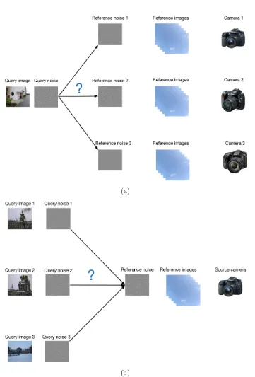
1.7 Use of SPN in source camera identification. (a) Identifying the source camera of a given image among candidate cameras and (b) Identifying the images taken by a camera among candidate images. . . 10
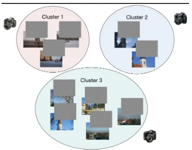
1.8 Use of SPN in image clustering. . . 12
1.9 Use of SPN in digital image forgery detection. . . 13
2.2 (a) A natural image, (b) noise residual obtained with the Mihcak
denoising filter [1, 2], (c) noise residual obtained with PCAI8 [4],
and noise residual extracted with the BM3D denoising filter [5]. Note
that we only show the noise residual extracted from the green channel,
because there is no much difference for the red and blue channels. . . 22
2.3 Neighborhood of the center pixel to be predicted. This figure is
ex-cerpted from [4]. . . 24
2.4 Simplified imaging pipeline of a typical digital camera. . . 25
2.5 The color-decoupled noise residual extraction process for the red
channel. This figure is excerpted from [6]. . . 26
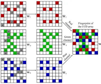
2.6 The construction of SPN using information from 3 color channels.
Block with @ refers to the pixel with large magnitude. This figure is
excerpted from [7]. . . 27
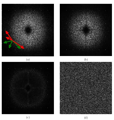
2.7 The logarithmic magnitude spectra of (a)R, (b) Rzm, (c)Rwf, and
Rph. . . 30
2.8 Sliding block shapes used for automatic ROI detection. This figure
is excerpted from [8]. . . 38
3.1 Filtering for the reference SPN of Canon PowerShot A400. (a)
Spec-trum of the original reference SPN, (b) specSpec-trum of the ZM filtered
reference SPN, (c) spectrum of the ZM + WF filtered reference SPN,
(d) spectrum of white noise. For visualization purposes, gamma
cor-rection with an exponent of 1.5 was applied to the spectra. . . 48
3.2 (a) Spectrum of the original reference SPN and the ones preprocessed
3.3 Estimated inter-class and intra-class PDFs ofρcalculated from SPNs
extracted from 3 different sizes of image blocks using BM3D. From
top to bottom, the rows show the distributions for image blocks sized
1024×1024, 256×256 and 64×64 pixels, respectively. From left to
right, the distributions are resulting from the original reference SPN
and the ones preprocessed by ZM, ZM+WF and SEA, respectively. . 62
3.4 Overall ROC curves of the combinations of different SPN
extrac-tors and preprocessing schemes (different columns) on different image
block sizes (different rows). From left to right, the columns show the
ROC curves for image blocks of 1024×1024, 256×256 and 64×64
pixels, respectively. Please refer to the last column for the legend
text, which is the same for the figures in the same row. . . 64
3.5 TPRs at the FPR of 1×10⁻³ for image blocks sized (a) 1024×1024
(b) 256×256 and (c) 64×64 pixels. . . 65
3.6 Ratios of the kappa statistic of SEA to that of ZM+WF for the cases
of estimating the reference SPN from JPEG images with a quality
factor 100 (first column) and JPEG images with the same quality
factor as the query images (second column). Bins are grouped
ac-cording to the quality factor of the query images, and each of the
six bins in the same group shows the ratio for one of the six SPN
extractors. From top to bottom, the rows show the results for image
blocks of 1024×1024, 256×256 and 64×64 pixels. . . 70
3.7 SNR for noise residual and the quantization noise introduced by
3.8 Spectra of the reference SPNs of the three special camera models.
From top to bottom, the rows show the spectra for Nikon CoolPix
S710, FujiFilm FinePix J50 and Casio EX-Z150, respectively. From
left to right, the columns show the spectra of the original reference
SPNs and the ones filtered by ZM, ZM+WF and SEA, respectively. 72
4.1 Flow chart of the proposed framework. . . 83
4.2 Probability density functions of the embedding error in pairwise
correlations ofD1 (a) andD3 (b). . . 98
4.3 ROC curves obtained by varying a threshold from −1 to 1 and
com-paring it to the pairwise correlations of camera fingerprints in dataset
D1 (a) andD3 (b). . . 99
4.4 Impact ofω on (a) the clustering performance and (b) the number of
images included in the final results. . . 100
4.5 How the score threshold ts and the size η of the minimal cluster
affect the clustering results. (a) Precision rates. (b) Recall rates. (c)
F1-Measures. (d) Number of clustered images. . . 101
4.6 Superiority of the potential-based eviction over the random eviction.
(a)c= 20. (b)c= 500. . . 103
4.7 Comparison of the effectiveness of thresholds. The first and second
rows show the results for two cases, i.e., cameras are of different
mod-els or the same model, respectively. From left to right, the columns
show the results for four sets of values, i.e., (nx = 1, ny = 10),
(nx= 10, ny = 30) and (nx= 30, ny = 50), respectively. . . 104
4.8 Running times and clustering qualities of different clustering
algo-rithms on datasets with various sizes. (a) Running time (in seconds).
5.1 How to determine the thresholds for given inter-camera and
intra-camera correlation distributions. . . 115
5.2 How preprocessing affects the correlation distribution p(x|h0) and
p(x|h1). . . 116
5.3 Predicted correlations obtained with the correlation predictor
pro-posed in [9] using 20480 image blocks of sized= 128×128 pixels for
(a) a Canon IXY500 and (b) a Canon IXUS 850IS. . . 117
5.4 An example of image inpainting. (a) Original image (b) Forged image.119
5.5 The square detection block across the non-tampered region Ωh1
i and the tampered region Ωh0
i . . . 120 5.6 How the correlation distribution changes as the detection block moves
across the boundary region. . . 123
5.7 15 paired groups for generating simulated image forgeries. . . 125
5.8 ROC curves obtained with different detection block sizes for different
forgery sizes. (a) Forgery size: 384×384, d=256×256. (b) Forgery
size: 256×256, d=256×256. (c) Forgery size: 128×128, d=256×256.
(d) Forgery size: 384×384, d=128×128. (e) Forgery size: 256×256,
d=128×128. (f) Forgery size: 128×128, d=128×128. (g) Forgery
size: 384×384, d=64×64. (h) Forgery size: 256×256, d=64×64. (i)
Forgery size: 128×128, d=64×64. . . 126
5.9 Forgery detection results for scaling (the first column),
copy-and-move (the second column) and cut-and-paste (the third row) forgery
using a detection block of 256×256 pixels. (a) Original image. (b)
Forged image. (c) Predicted correlation field. (d) Actual correlation
field. (e) Detection result by CFAR. (f) Refined detection result by
5.10 Forgery detection results for scaling (the first column),
copy-and-move (the second column) and cut-and-paste (the third row) forgery
using a detection block of 128×128 pixels. (a) Original image. (b)
Forged image. (c) Predicted correlation field. (d) Actual correlation
field. (e) Detection result by CFAR. (f) Refined detection result by
our proposed algorithm. . . 130
5.11 Forgery detection results for scaling (the first column),
copy-and-move (the second column) and cut-and-paste (the third row) forgery
using a detection block of 64×64 pixels. (a) Original image. (b)
Forged image. (c) Predicted correlation field. (d) Actual correlation
field. (e) Detection result by CFAR. (f) Refined detection result by
our proposed algorithm. . . 131
5.12 ROC curves for three forged images obtained with different detection
block sizes. (a) Image 1, d=256×256. (b) Image 2, d=256×256.
(c) Image 3, d=256×256. (d) Image 1, d=128×128. (e) Image 2,
d=128×128. (f) Image 3, d=128×128. (g) Image 1, d=64×64. (h)
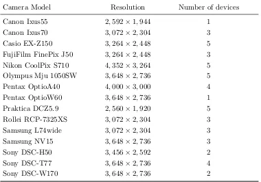
3.1 49 cameras involved in the creation of the images in the Dresden
database . . . 57
3.2 6 cameras involved in the creation of the images in our own database 58 3.3 Kappa statistics for 1024×1024 image blocks . . . 67
3.4 Kappa statistics for 256×256 image blocks . . . 67
3.5 Kappa statistics for 64×64 image blocks . . . 68
3.6 Kappa statistics for Nikon CoolPix on 256×256 image blocks . . . . 75
3.7 Kappa statistics for FujiFilm FinePix J50 on 256×256 image blocks 75 3.8 Kappa statistics for Casio EX-150 on 256×256 image blocks . . . . 76
3.9 Running time comparison (ms) . . . 76
4.1 Clustering results on the generated datasets . . . 106
4.2 Comparison of 4 different clustering algorithms on 4 different datasets: (a)D1, (b)D2, (c)D3, and (d)D4. . . 108
5.1 AUCs for forgeries of size 384×384 pixels. . . 126
5.2 AUCs for forgeries of size 256×256 pixels. . . 127
5.3 AUCs for forgeries of size 128×128 pixels. . . 127
5.4 AUCs on image 1. . . 132
5.5 AUCs on image 2. . . 132
Introduction
1.1
Digital Image Forensics
Advances in digital imaging technologies have led to the development of low-cost
and high-quality digital imaging devices, such as camcorders, digital cameras,
scan-ners and built-in cameras of smartphones. The ever-increasing convenience of image
acquisition has facilitated the distribution and sharing of digital images, and bred
the pervasiveness of powerful image editing tools, allowing even unskilled persons
to easily manipulate digital images for malicious or criminal ends. Under the
cir-cumstances where digital images serve as critical evidence for news photography,
scientific discovery, law enforcement, etc., maliciously manipulated images may lead
to serious consequences.
(a) (b)
Figure 1.1: Misleading report on Luxor massacre by the Swiss tabloid Blick in 1997. (a) Altered image. (b) Original image.
Fig. 1.1(a) shows a image posted by the Swiss tabloid Blick after 62 tourists
(including 36 Swiss tourists) were killed in a terrorist attack at the temple of
Hat-shepsut in Luxor Egypt1. A puddle of water in the original image (Fig. 1.1(b)) was
1
digitally altered to appear as blood flowing from the temple. Fig. 1.2(a) shows the
American astronaut Stephen Robinson on a spacewalk in front of the Canadarm22.
Unfortunately, The Economist pointed out that the Canadian logo visible on the
arm in the image was crudely composited, because the background color and
tex-ture of the logo clearly does not match the arm. In fact, it was discovered that the
original image (Fig. 1.2(b)) without any Canadian logo was captured by NASA.
The composite image was used by several Canadian government websites to
pro-mote Canada’s involvement with the International Space Station. Tampered image
presented as evidence in the law enforcement system can be used to frame innocent
people unjustly. Kanhaiya Kumar, a student leader at India’s Jawaharlal Nehru
University, was arrested on sedition charges in the midst of a variety of contested
images and video clips which claim to show him advocating for the disintegration of
India3. One image (Fig. 1.3(a)) that circulated widely on social media shows Kumar
speaking in front of a map showing a divided India, in which portions of Kashmir
and Gujarat were annexed to Pakistan. However, in the original, undoctored image
(Fig. 1.3(b)), Kumar is actually speaking in front of a blank background.
(a) (b)
Figure 1.2: An example of forged images used in the scientific discovery field. (a) A composite image used by several Canadian government websites to promote Canada’s involvement with the International Space Station and (b) the original image.
As can be seen in the above examples, we are now living in a world of “seeing
2http://pth.izitru.com/2014_10_00.html
3
(a) (b)
Figure 1.3: An example of forged images used by law enforcement. (a) A doctored image showing Kumar speaking in front of a map of a divided India and (b) the original image.
is not believing”. Digital images can be easily forged with increasingly powerful and
user-friendly image editing software without leaving visible traces. The increasing
appearance of digitally altered forgeries on the Internet and in mainstream media
is casting doubt on the integrity of digital images. Untrustworthy images have
challenged the public credibility, judicial impartiality, academic morality,
journal-istic integrity, etc., therefore, it is important and necessary to carry out research
on forensic technologies that can verify the originality, integrity and authenticity of
digital images.
Digital image forensics research aims at revealing underlying facts about a
suspicious image [10]. It is not limited to exposing image forgeries, as shown in the
above examples, but involves a wide range of investigations. It is intended to answer
the questions including but not limited to:
• Which device among the candidates was used to capture the image in question?
• Which images among the candidates were captured by the same source device
X?
• Is this image an original image or has it been tampered with for ulterior
• What parts of the image has been forged and up to what extent?
• What is the processing history of the image?
1.1.1 Active Digital Image Forensics
To determine the originality, integrity and authenticity of a digital image, a
straight-forward way is to insert extra digital watermark [11–17] or signature [18–21] into
the image when it is created. The changes in the image are then detected by
re-covering and checking the embedded digital signature or watermark. For example,
Fridrich and Goljan [13] proposed two techniques to embed an image in itself both
for protecting the image content and for authentication. In [14], a semi-fragile
wa-termarking method was proposed for the automatic authentication and restoration
of the image content using irregular sampling. In spite of the effectiveness of these
active techniques, they can only be applied when the image is protected at the
ori-gin. Nowadays, the majority of images do not contain a digital watermark/signature
mainly due to the following reasons:
• Camera manufacturers have to devise extra digital watermark/signature
em-bedding components in the camera, so only some high-end cameras have
wa-termark embedding features.
• The embedded watermark/signature may degrade the image quality and
sig-nificantly reduce the market value of cameras featuring watermark/signature
embedding capability.
• The successful implementation of watermark-based protection requires close
collaborations among publishers/manufaturers, investigators and potentially
trusted third-party organizations. This limits the adoption of digital
1.1.2 Passive Digital Image Forensics
Compared to the above active forensic technology, passive image forensic
technolo-gies require no collaboration of users and is based on the inherent patterns in the
image itself. Most image manipulations do not leave noticeable visual artifacts, but
they do inevitably change the statistical characteristics of the manipulated image.
Passive forensic technologies verify the originality, integrity and authenticity of
im-ages through detecting the changes of statistical image characteristics. It does not
need to insert extra information in the image and there is no special requirement on
the imaging hardware. Therefore, there has been growing interest in passive forensic
techniques. Over the past few years, the research on passive image forensics mainly
has focused on the following three directions [10]:
1. Image source identification to determine the data acquisition device that
gen-erates one image. It identifies the source device at four different accuracy
levels:
• Device type: For example, is the given image generated by a camera or
a scanner?
• Device brand: For example, is the given image taken by a Canon Camera
or a Nikon camera?
• Device model: For example, is the given image taken by Canon 450D or
Canon IXUS70?
• Individual device: For example, is the give image taken by this specific
camera or another camera?
2. Discrimination of synthetic images images from real images to identify
computer-generated images which do not depict a real-life occurrence. As computer
graphics technology develops, it becomes increasingly difficult to distinguish
been a trend of presenting synthetic images as real images or augmenting the
computer-generated virtual scenes with real scenes to deceive the viewer.
3. Image forgery detection to determine whether or not an image has undergone
any form of modification or processing after it was originally captured. It also
uncovers the parts of the given image that have been altered and up to what
extent.
As shown in Fig. 1.4, passive image forensics can be divided into three
categories based on the characteristics of the used images:
1. Passive image forensics based on natural image statistics: For example, Lyn
and Farid [22] decomposed each color channel of a color image using the
sep-arable quadrature mirror filters (QMFs) [23, 24], then calculated the mean,
variance, skewness, and kurtosis of the subband coefficient histograms at each
orientation and scale. They also considered the linear prediction errors of
co-efficient magnitudes between adjacent pixels, scales, directions and color
chan-nels. These features were input into a linear discrimination analysis (LDA) or
a nonlinear support vector machine (SVM) classifier to differentiate between
photorealistic (computer-generated) and photographic images. In [25],
Khar-razi et al. proposed 34-dimensional image features, including the mean value
of the RGB channels (3 features), the correlation pairs between RGB channels
(3 features), neighbor distribution center of mass for each of the 3 channels (3
features), RGB pairs energy ratio (3 features), wavelet domain statistics for 3
sub-bands in 3 color channels (9 features) as well as 13 image quality metrics
features, to distinguish the images taken by different cameras.
2. Passive image forensics based on traces left by specific image manipulations:
A counterfeiter has to apply one or more image manipulations to forge an
image. A specific image manipulation will leave some specific patterns in
forgeries by looking for the traces left by specific image manipulations such as
double JPEG compression [26, 27], resampling [28, 29], contrast enhancement
[30–34], etc. It also includes the methods that detect the duplicated image
regions [35–37] or the inconsistent lighting conditions [38, 39] introduced by
copy-and-paste image forgery.
3. Passive image forensics based on consistent characteristics introduced by
var-ious imaging devices or different hardware or software processing components
in the imaging pipeline: Shown in Fig. 1.5 is the simplified imaging pipeline in
digital camera. Each processing component in the pipeline will leave specific
and consistent characteristics in the resulting image. Therefore, by detecting
the presence of the consistent characteristics introduced by imaging device, we
can trace back to the image source. Likewise, we can also uncover the image
forgery by detecting the absence of those consistent characteristics. The
con-sistent characteristics include the characteristics left by lens distortion [40],
color filter array (CFA) interpolation (or demosaicing) [28, 41], camera
re-sponse function (CRF) [41–43], JPEG artifacts [44] and sensor pattern noise
(SPN) [1, 3, 9, 45].
Passive digital image forensics
Based on natural image statistics
Based on traces left by specific image manipulations
Based on consistent characteristics introduced by imaging
device
Figure 1.5: Simplified imaging pipeline in a typical digital camera.
1.2
Sensor Pattern Noise
As one of the most promising passive image forensic approaches, methods based on
sensor pattern noise (SPN) have attracted increasing attention in recent years. As
shown in Fig. 1.6, sensor pattern noise consists of two main components. One is
the dark signal non-uniformity (DSNU)4 (or dark current noise as it is more
com-monly referred to as), which is the pixel-to-pixel differences when the sensor array
is not exposed to light. The dominant component in SPN is the photo response
non-uniformity (PRNU) noise, which arises primarily from the manufacturing
im-perfections and the inhomogeneity of silicon wafers during the sensor manufacturing
process. It is a powerful forensic tool due to its 1) uniqueness to individual device,
2) stability against environmental conditions and 3) robustness to some common
image processing operations. Therefore, it can be considered as the fingerprint of
imaging devices and has been widely and successfully applied in the filed of digital
image forensics. In the following subsections, source camera identification, image
clustering and image forgery detection based on SPN will be introduced.
4
Pattern noise
DSNU
PRNU
Figure 1.6: Pattern noise of imaging sensors [1].
1.2.1 Source Camera Identification Based on SPN
One challenging problem of multimedia forensics is source camera identification
(SCI). The task of SCI is to reliably match a particular digital image with its source
device. SPN is considered as the fingerprint of source camera left in every image
taken by the source camera, so it can be used for tracing back to the source device
of an image. Shown in Fig. 1.7(a) is the process of SPN-based source camera
identification. Firstly, a reference SPN is constructed for every candidate camera by
averaging the noise residues extracted from a collection of images captured by the
candidate camera. The images used for constructing the reference SPN are usually
those with high intensity and low texture, e.g., blue sky images, because the SPN is
better preserved in them. To determine the source camera that has taken a query
image among all candidate cameras, the noise residue of the query image (or query
SPN) is extracted and compared with the reference SPN. If the highest similarity
is higher than a predefined threshold, the query image is deemed to be taken by
the camera with the highest similarity. Another forensic scenario is shown in Fig.
1.7(b), where SPN is used for identifying the image among candidate images taken
(a)
[image:30.595.143.504.105.638.2](b)
in minor points. In this scenario, as long as the similarity between the query SPN
and the reference SPN is high enough, the query image is considered to be captured
by the camera.
1.2.2 Image Clustering Based on SPN
In the above application of SPN in source camera identification, a set of images taken
by the same camera are required for the construction of the reference SPN. This
requirement can be easily fulfilled when the camera is available to the investigators.
However, in many real-world scenarios, only a set of images are available, but
with-out any information abwith-out the source cameras. In such circumstances, sometimes
it is still desirable to be able to cluster the images into a number of groups, each
including the images acquired by the same camera. Take Internet child pornography
for example, lots of illegal images can be confiscated from pornographic website, but
the cameras which have taken these images are not available to the forensic
investi-gators. If we can cluster these images into a number of groups, each including the
images acquired by the same camera, we are able to associate different crime scenes
and would be in a better position to link the evidence to the seized hardwares that
are owned by the suspects in the future. As shown in Fig. 1.8, this task can be
accomplished by resorting to the use of SPNs extracted from the images. By
clus-tering the SPNs, the corresponding images taken by the same camera are grouped
into the same group.
1.2.3 Image Forgery Detection Based on SPN
Sensor pattern noise (SPN) can be considered as a spread-spectrum watermark
embedded in every image taken by the source imaging device. Therefore, it can also
be used for localizing the forgeries in digital images. However, since SPN, by its
very nature, is a very weak noise-like signal, its reliable detection requires jointly
Figure 1.8: Use of SPN in image clustering.
in Fig. 1.9, the SPN extracted from the image in question is compared with the
reference SPN in a block-wise manner. If their similarity (usually normalized cross
correlation), which serves as a decision statistic, is below a pre-determined threshold
(e.g., by Neyman-Pearson criterion), the center pixel in the block is declared as
forged. This method exposes the image forgery by detecting the absence of SPN
irrespective of the specific type of forgery, it therefore arouses wide attention of the
researchers in the field of digital forensics.
1.3
Main Contributions
Digital image forensics is a broad area and includes research spanning a range of
directions. In this thesis, our research on digital image forensics is narrowed down
Figure 1.9: Use of SPN in digital image forgery detection.
clustering and image forgery detection. The major contributions we have made are
summarized in detail as follows.
1. Although SPN has been proven to be an effective means to uniquely
iden-tify digital cameras, some non-unique artifacts, shared amongst cameras
sub-jected to the same or similar in-camera processing procedures, often give rise
to false identifications. We propose a novel preprocessing approach, i.e.,
spec-trum equalization algorithm (SEA) in Chapter 3, that equalizes the magnitude
spectrum of the reference SPN through detecting and suppressing the peaks
according to the local characteristics. It aims at removing the interfering
pe-riodic artifacts and therefore reduces the false identification rate.
2. The challenges of clustering large-scale camera fingerprints come from the
large-scale and high-dimensional nature of the problem. The difficulties can
be further aggravated when the number of classes is much higher than the
av-eraged class size, which is not uncommon in many practical scenarios. We
propose an efficient clustering framework for large-scale device fingerprint
database in Chapter 4. The framework works in an iterative way and
uti-lizes both the dimension reduction technology and divide&conquer strategy
easily parallelized and adapted to very large-scale camera fingerprints
cluster-ing tasks.
3. As demonstrated in Fig. 1.9, the reliable detection of SPN for exposing image
forgery requires the algorithm to work in block-wise manner. However, when
the detection block falls near the boundary of the tampered and the
non-tampered regions, the decision statistic becomes a weighted average of two
different contributions and may lead to a high false acceptance rate (FAR)
(i.e., misidentifying a tampered block as non-tampered). We propose a
re-fining algorithm to alleviate the missing detection problem in Chapter 5. We
model how the decision statistic changes as the detection block is placed across
the boundary of two different regions (i.e., tampered and non-tampered) and
adjust the decision threshold accordingly to achieve a more satisfactory
detec-tion.
1.4
Outline of Thesis
This chapter briefly introduces the background of digital image forensics and how
sensor pattern noise can be used for identifying source camera, clustering images
and exposing image forgeries. The rest of this thesis is organized as follows.
Chapter 2 first categories the interferences introduced in the imaging pipeline
that affect the quality of the estimated SPN and introduces the approaches that
aim at alleviating or eliminating the effect of the interferences to improve the
per-formance of SPN based source camera identification. It then revisits the related
work on image clustering based on camera fingerprint and points out the challenges
of clustering large-scale image databases that have not yet been addressed by the
existing methods. Literature on SPN based image forgery detection will also be
reviewed in the last section of this chapter.
SPN preprocessing schemes. It then presents the details of a novel preprocessing
scheme, spectrum equalization algorithm (SEA), that overcomes the limitations of
existing approaches. Combined with 6 state-of-the-art SPN extraction methods, the
proposed preprocessing scheme is evaluated with comprehensive experimental results
and analysis on the Dresden image database for both the general and special cases.
Finally, it also gives the comparison of running times among different preprocessing
schemes and similarity measurements.
Chapter 4 introduces our proposed clustering framework for large-scale
cam-era fingerprint databases step by step, including data preparation, coarse clustering,
fine clustering, centroid attraction and post processing. It also discusses the
param-eter selection and time complexity. Finally, it validates the capability of clustering
large-scale databases and the advantage of the proposed framework over other
state-of-the-art clustering algorithms with extensive experimental results.
Chapter 5 first introduces the missing detection problem of SPN based image
forgery detection along the boundary between the forged and non-forged areas. It
then models the correlation distribution in the problematic area and proposes to
adjust the threshold accordingly to alleviate the missing detection problem. In this
chapter, the effectiveness of the algorithm is verified via three realistic image forgery
detection examples.
Chapter 6 summarizes this thesis. Several key challenges we are confronted
Literature Review
2.1
Source Camera Identification
Sensor Pattern Noise (SPN) has attracted much attention from researchers in the
area of digital forensics since it was proven to be an effective and robust device
fingerprint in [1]. One of the important applications of SPN is source camera
iden-tification (SCI), which is about identifying the source camera of a given image from
candidate cameras. The typical process of using SPN for SCI is as follows. A
refer-ence SPNRis first constructed by averaging the noise residual Wi extracted from
theith image of theN images taken by the same camera:
R= 1
N
N
X
i=1
Wi. (2.1)
The similarity between the reference SPN R and the query noise residue W is
measured by the normalized correlation coefficient (NCC)ρ:
ρ(R,W) =
Pm
i=1
Pn
j=1(W[i, j]−W)(R[i, j]−R)
kW−Wk · kR−Rk , (2.2)
where k · k is the L2 norm, R and W are of the same size m×n, and R and W
are the arithmetic mean of R and W, respectively. Suppose the reference SPN of
camerac is Rc, the task of SCI is then achieved by identifying camerac∗ with the
maximal NCC value that is greater than a predefined threshold τρ as the source
device of the query image, i.e.,
c∗ = argmax c∈C
whereC is the set of candidate cameras.
However, the correlation-based detection of SPN heavily relies upon the
qual-ity of the extracted SPN, which can be severely contaminated by different
interfer-ences. In the following subsections, the interferences that may degrade the quality
of SPN and the approaches used to alleviate or eliminate the interferences will be
discussed.
2.1.1 Scene Details
SPN is a weak noise-like signal, so its estimation is usually based on the the noise
residualW, where the image content is significantly suppressed. The noise residual
W of an imageI is formulated as
W=I−F(I), (2.4)
whereF(·) is a denoising filter. The widely used denoising filter for SPN extraction
is the wavelet-based technique proposed by Mihcak et al. [2]. As described in [1], it
works as follows
1. Calculate the four-level wavelet decomposition of the noisy image with the
8-tap Daubechies QMF. Denote the horizontal, vertical, and diagonal subbands
ash[i, j],v[i, j] andd[i, j], where [i, j] runs through an index setJthat depends
on the decomposition level. We only show the operations for h[i, j] in the
following two steps, because the operations onv[i, j] andd[i, j] are exactly the
same.
2. Estimate the local variance of the original noise-free image for each wavelet
a squarew×wneighborhood Nw, i.e.,
ˆ
σ2[i, j] = min w∈{3,5,7,9}
max0, 1 w2
X
[k,l]∈Nw
h2[k, l]−σ02
, (2.5)
whereσ2
0 is the overall variance of additive Gaussian white noise to be removed
and is usually set to 4 or 9 for high-quality images.
3. The denoised wavelet coefficients are obtained suing the Wiener filter
ˆ
h[i, j] =h[i, j] σˆ
2[i, j]
ˆ
σ2[i, j] +σ2 0
. (2.6)
4. Repeat above 3 steps for each level and apply the inverse wavelet transform
to the denoised wavelet coefficients to obtain the denoised image.
Shown in Fig. 2.1(a) and Fig. 2.1(b) are an image of natural scene and the
noise residual extracted with the Mihcak denoising filter [1, 2]. As can be seen, the
noise residual contains strong scene details, especially in the edge areas, because
scene details account for part of the components of I and their magnitude is far
greater than that of SPN [3].
Many efforts have been devoted to suppressing scene details in the noise
residual to obtain SPN of higher quality. In [3], Li proposed 5 models to attenuate
scene detail by assigning less significant weighting factors to the strong components
of SPN in the Digital Wavelet Transform (DWT) domain. The underlying rationale
is based on the hypothesis that the stronger a signal component in noise residual
W is, the more likely that it is associated with strong scene details, and thus the
less trustworthy the component should be. The enhanced noise residual of the image
(Fig. 2.1(a)) is shown in Fig. 2.1(c), where the magnitudes of strong edges have
been suppressed.
(a) (b) (c)
Figure 2.1: (a) A natural image, (b) noise residual obtained with the Mihcak de-noising filter [1, 2], and (c) noise residual enhanced using Model 3 with parameter 6 proposed in [3]. Note that the noise residual is extracted only from the green channel.
is the PRNU noise. So in [9], noise residualW is modeled as
W = IK+Ξ, (2.7)
whereIis the observed image,Kis the zero-mean like multiplicative factor
responsi-ble for PRNU, andΞstands for other noises including the interferences from image
content, dark current noise, shot noise, and the errors introduced by the denoising
filter. Equation (2.7) indicates that to obtain better estimation of SPN, the
lumi-nance I should be as high as possible but not saturated because saturated pixels
carry no information about the PRNU factor [9]. Another observation in Equation
(2.7) is that high variation in Ξ introduces strong interference to IK. Therefore,
SPN is better preserved in smooth areas (i.e., with lower variance). Based on the
two insights that stems from Equation (2.7), some works improve the performance
of source camera identification by taking into consideration pixel intensity and
spa-tial variation. For example, a weighting scheme based on the image gradient was
proposed in [46]. The weightw(p) for each pixelp is calculated as
w(p) =G(σ)∗ 1 1 +k∇Ipk
where G(σ) is a Gaussian kernel and ∇ denotes the gradient operator. While in
[47], both the image intensities and image textures were considered. The authors
classified the image pixels into four classes:
• Class 1: Low brightness, Low texture
• Class 2: Medium brightness, High texture
• Class 3: High brightness, Low texture
• Class 4: Saturated brightness, Medium texture.
They found that Class 3 is the best class in the sense of increasing the
intra-camera similarities and decreasing the inter-intra-camera similarities. A more
sophisti-cated weighting scheme that formulates the relationship between the image features
(related with image intensity and texture) and the correlation values was proposed
in [48]. The image features are defined as
fbi= 1 |Bb|
X
i∈Bb
Ip
fbt = 1 |Bb|
X
i∈Bb
1 1 + var3(Ip)
,
(2.9)
where Bb is the image block, |Bb| is the cardinality of Bb, Ip is the intensity of
the image at pixel p, and var3(Ip) is the variance of Ip in a 3×3 neighborhood.
The 2-dimensional features are extracted from each of the M 128×128-pixel image
blocks cropped from a set of training images (100 training images for each camera
were used in [48]). Then the kernel principal component analysis (KPCA) [49] was
used to predict the correlationsρbetween the reference SPN and the SPN extracted
from training blocks:
ˆ
ρ=Hθ, (2.10)
whereHconsists of the principal components of Φ(X), which defines the non-linear
be considered as the projected data of X via KPCA, and θ can be estimated by
applying the lease square estimator (LSE)
θ =HTH−1HTρ. (2.11)
A low predicted correlation ˆρ means a large amount of image content is left in the
noise residue. On the other hand, a large predicted correlation means that the
region does not suffer from image content effect. Hence, the predicted correlation
can be used to weight the center pixel of the extracted SPN [48]. While all the
afore-mentioned schemes aim at weighting the query SPN, a weighted averaging
scheme [50] was proposed for the estimation of the reference SPN. Specifically, the
equal weighting factor 1/N in Equation (2.1) is replaced with
wi= 1 σ2 i XN m=1 1 σ2 m −1
, i= 1, ..., N, (2.12)
whereσ2
i is the variance of undesirable noise, i.e.,
σi2=
PL
j=1(ni[j]−ni)2
L
ni =Wi−W
ni =
PL
j=1ni[j]
L
W=
PN
i=1Wi
N .
(2.13)
Note thatL is the length of samples (i.e., the image size). As reported in [50],
sig-nificant performance improvements can be achieved by adopting this new weighting
scheme.
Since the denoising filterF(·) in Equation (2.4) plays a key role in preventing
the scene details from propagating to W, a straightforward idea is to use more
(a) (b)
[image:42.595.126.516.110.504.2](c) (d)
Figure 2.2: (a) A natural image, (b) noise residual obtained with the Mihcak de-noising filter [1, 2], (c) noise residual obtained with PCAI8 [4], and noise residual extracted with the BM3D denoising filter [5]. Note that we only show the noise residual extracted from the green channel, because there is no much difference for the red and blue channels.
i.e., block matching and 3D filtering (BM3D), to obtained the noise residual from
images [5] BM3D works by grouping 2D image patches with similar structures into
3D arrays and collectively filtering the grouped image blocks. The sparseness of the
representation due to the similarity between the grouped blocks makes it capable of
better separating the true signal and noise. Compared to the noise residual obtained
are removed in the noise residual obtained with BM3D [5]. Wu et al. [51] proposed
another SPN extractor, edge adaptive SPN predictor based on context adaptive
interpolation (PCAI), to suppress the effect of scenes and edges. SupposeIp is the
pixel value to be predicted at pixel p, then the predicted pixel value is formulated
as
ˆI(p) =
mean(t), (max(t)−min(t)≤20)
(n+s)/2, (|e−w| − |n−s|>20)
(e+w)/2, (|n−s| − |e−w|>20)
median(t), (otherwise),
(2.14)
where t = [n, s, e, w]T is the four-neighboring pixels of p, as shown in Fig. 2.3.
An extension of this method is to make use of all the eight neighboring pixels
t0 = [n, s, e, w, en, es, wn, ws]T, as proposed in [4], where ˆI(p) is formulated as
ˆ I(p) =
mean(t0), (max(t0)−min(t0)≤20)
(n+s)/2, (|e−w| − |n−s|>20)
(e+w)/2, (|n−s| − |e−w|>20)
(es+wn)/2, (|en−ws| − |es−wn|>20)
(en+ws)/2, (|es−wn| − |en−ws|>20)
median(t0), (otherwise).
(2.15)
Finally, a pixel-wise Wiener filter will be performed on the difference between the
original and the predicted image,D=I−ˆI, to obtain the noise residual
W[i, j] =D[i, j] σ
2 0
ˆ
σ2[i, j] +σ2 0
, (2.16)
where
ˆ
σ2[i, j] = max0, 1 w2
X
[k,l]∈Nw
Figure 2.3: Neighborhood of the center pixel to be predicted. This figure is excerpted from [4].
σ2
0 andwhave the same meanings as in Eq. 2.5. In both [51] and [4], the sizewof the
local neighborhood andσ2
0 are set to 3 and 9, respectively. Throughout this thesis,
the method in [4] will be referred to as PCAI8 and used to represent this line of
work. The noise residual extracted with PCAI8 is shown in Fig. 2.2(d). Surprisingly,
although PCAI8 was declared to have better performance than the Mihcak filter and
BM3D in [4], the scene details are more pronounced in Fig. 2.2(d).
2.1.2 Demosaicing
In digital cameras, the imaging sensor is probably the most expensive component.
Therefore, to reduce the costs and increase the sales, most consumer digital cameras
are equipped with only one sensor and an associated color filter array (CFA) to
capture all necessary colors at the same time. Fig. 2.4 shows the simplified imaging
pipeline, where the most widely used Bayer CFA is placed on top of a CCD sensor.
For each pixel, only one color component passes through the CFA and consequently
forms a monochrome image. To recover the full-color image from the mosaic-like
monochrome image captured by the sensor, a demosaicing, or CFA interpolation,
process needs to be devised to estimate the missing color components. However,
the estimated color components are not directly acquired by physical hardware and
carry interpolation noises. We expect that the PRNU extracted from the physical
that from the artificial channels, which carry interpolation noise. Therefore, it is
expected that the SPN extracted from the “physical” components, which are free
from interpolation noise, should be more reliable than that from the “artificial”
components.
CFA + CCD
Demosaicking
Lens
Postprocessing Scene
Figure 2.4: Simplified imaging pipeline of a typical digital camera.
To address this issue, Li and Li proposed a Color-Decoupled PRNU
(CD-PRNU) extraction method in [6], which first decomposes each color channel into 4
sub-images and then extracts the PRNU noise from each sub-image. The PRNU
noise patterns of the sub-images are then assembled to get the CD-PRNU. Fig.
2.5 shows the noise residual extraction process for the red color channel, similarly
for the green and the blue channels. This method can prevent the interpolation
noise from propagating into the physical components, thus improving the accuracy
of device identification and image content integrity verification [6]. In [7], Hu et
al. proposed to exploit the CFA structure to make better use of the information
from all the 3 color channels. The process is depicted in Fig. 2.6: First, the large
components in the noise residual of each color channel are selected based on their
work in [52] (the first column of Fig. 2.6). Second, only the physical components
(i.e., the components that are not in the interpolated positions) are kept, as shown
in the second column of Fig. 2.6. Finally, the remaining components in 3 color
channels are combined to acquire the camera fingerprint (the last column of Fig.
2.6). However, the CFA structure is usually unknown in practice, so they compared
Figure 2.5: The color-decoupled noise residual extraction process for the red channel. This figure is excerpted from [6].
position on other color channels. If it is the largest component, then it is kept,
˜
Wg,
˜
Wg =
˜
Wg, ifg= argmax x∈{r,g,b}|
˜
Wx|
0, otherwise.
(2.18)
In this way, the impact of demosaicing on the extracted noise residual has
been reduced.
Wr
Wg
Wb W˜b
˜
Wg
˜
Wr
[image:47.595.149.486.248.530.2]W
Figure 2.6: The construction of SPN using information from 3 color channels. Block with @ refers to the pixel with large magnitude. This figure is excerpted from [7].
2.1.3 Periodic Artifacts
For the task of source camera identification, some periodic artifacts, shared amongst
cameras subjected to the same or similar periodic in-camera processing procedures,
are not unique to the sensor. The SPN estimated from two different cameras may
reliability of identification system. Non-unique periodic artifacts can be summarized
as follows:
• CFA interpolation artifacts: A typical CFA interpolation is accomplished
by estimating the missing components from spatially adjacent pixels according
to the component-location information indicated by a specific CFA pattern.
As CFA patterns form a periodic structure, measurable offset gains will result
in periodic biases in the interpolated image [9]. The periodic biases manifest
themselves as peaks in the DFT spectrum, and the locations of the peaks
depend on the configuration of the CFA pattern.
• JPEG blocky artifacts: In JPEG compression, non-overlapping 8×8-pixel
blocks are coded with DCT independently. So high JPEG compression causes
blocky artifacts, which manifest themselves in the DFT spectrum as peaks in
the positions (U
8u,
V
8v), where U and V are the sizes of the spectrum, and
u, v∈ {0,1, ...,7}.
• Diagonal artifacts: As reported in [53], unexpected diagonal artifacts were
observed for the reference SPN of Nikon CoolPixS710. Although the cause is
yet to be investigated, the artifacts are reflected in the spectrum as peaks in
the positions corresponding to the row and column period introduced by the
diagonal artifacts.
Some works have been proposed to suppress these periodic artifacts. Chen et
al. preprocessed the reference SPNRby zero-meaning (ZM) operation and Wiener
filtering (WF) in the DFT domain in [9]. In the zero-meaning operation, column
averages ofR are subtracted from each pixel in each column and then row averages
are subtracted from every pixel in the row to obtain the zero-meaned signalRzm. In
the subsequent WF operation, Rzm is further processed in the DFT domain using
a Wiener filter:
Rwf = Real
F−1 D·|D| − W(|D|, σ2)
|D|
where Real(·) returns the real part of input, F(·) is the DFT, W(·) is the Wiener
Filter,D=F(Rzm),|D|is the magnitude ofD, andσ2= M N1 Pi,jRzm[i, j]. In [45],
Kang et al. only kept the phase component of the noise residual and constructed a
reference phase SPN to enhance the performance of SCI:
Rph= Real
F−1
PN
i=1Wφi
N
, (2.20)
whereF−1(·) is the inverse DFT andW
φiis phase-only component of noise residual
Wi, i.e.,
Wφi= F
(Wi)
|F(Wi)|
, i= 1,2, ..., N. (2.21)
The underlying rationale is that the SPN (noise residue) is usually modeled as an
additive white Gaussian noise (AWGN) in its extraction process, it is reasonable
to assume the camera reference SPN to be a white noise signal with flat frequency
spectrum to remove the impact of the contamination in the frequency domain [45].
Only keeping the phase components whitens the noise residual in the frequency
domain and helps to remove the periodic artifacts.
The above-mentioned methods are claimed to be effective in suppressing the
periodic artifacts. We conducted experiments on one Olympus Mju 1050SW, which
suffers severely from the periodic artifacts, to see their performances on
suppress-ing the unwanted periodic artifacts. 50 flat field (i.e., intensities are approximately
constant) images were used for estimating the reference SPN. The size of reference
SPN is 256×256 pixels and each noise residual used for reference estimation was
extracted from the green channel using the Mihcak denoising filter [1]. The
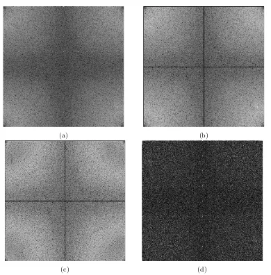
logarith-mic magnitude spectrum ofR,Rzm,Rwf, and Rph are shown in Fig. 2.7(a)-2.7(d).
As can be seen, compared toR, the DC components ofRzm are completely removed,
andRwfandRphare significantly whitened. However, the “white” points (peaks) in
the spectrum, which are related with the periodic artifacts, are clearly shown in the
(a) (b)
[image:50.595.128.518.109.505.2](c) (d)
Figure 2.7: The logarithmic magnitude spectra of (a)R, (b)Rzm, (c)Rwf, andRph.
in depth in Chapter 3.
Another set of approaches attempts to suppress the periodic artifacts through
the use of more sophisticated detection statistics or similarity measurements.
Gol-jan [54] proposed the peak-to-correlation energy (PCE) measure to attenuate the
influence of periodic noise contaminations
PCE(R,W) = C
2
RW[0,0] 1
M N−|A| P
[k,l]∈A/ CRW2 [k, l]
, (2.22)
between R and W, A is a small area around (0,0), and |A| is the cardinality of
the area. Later in [45], Kang et al. proposed to use the correlation over circular
cross-correlation norm (CCN) to further decrease the false-positive rate:
CCN(R,W) = q CRW[0,0]
1
M N−|A| P
[k,l]∈A/ CRW2 [k, l]
, (2.23)
where all the symbols have the same meanings as in Equation (2.22). Actually CCN
shares the same essence as the signed PCE (SPCE) [55, 56]
SPCE(R,W) = sign(CRW[0,0])C
2
RW[0,0] 1
M N−|A| P
[k,l]∈A/ CRW2 [k, l]
, (2.24)
where sign(·) is the sign function, and all the other symbols have the same meanings
as in Equation (2.22). Note that the above-mentioned approaches can be combined
for additional performance gains. For instance, one can apply ZM and WF
opera-tions on the reference SPN extracted with BM3D or PCAI algorithm, and enhance
the query noise residual with the help of Li’s models [3], and finally choose SPCE
or CCN as the similarity measurement to identify the source camera.
2.2
Image Clustering Based on SPN
As described in the last section, to determine the origin of a given image among
candidate cameras, a reference SPN is constructed for each candidate camera by
averaging the noise residues extracted from a set of images taken by the camera.
The given image is deemed to be taken by the camera associated with the detected
SPN in the image. In this case, a set of images taken by the same camera are
required for the construction of the reference SPN. This requirement can be easily
fulfilled when the camera is available to the investigators. However, in many
real-world scenarios, only a set of images are available, but without any information
are confiscated from pornographic websites, but the cameras which have been used
to take these images are not available to the forensic investigators. In some forensic
circumstances, it is necessary to cluster the images into a number of groups, each
including the images acquired by the same camera, so that the forensic investigators
are able to associate different crime scenes and would be in a better position to link
the evidence to the seized hardwares that are owned by the suspects. This task
can be accomplished by clustering the images based on the SPNs extracted from
the images. While several methods have been proposed for clustering the camera
fingerprints, their applicability is restricted to small datasets mainly due to the
large-scale and high-dimensional nature of the problem.
2.2.1 Markov Random Field Based Method
One of the first works dedicated to clustering camera fingerprints into a number of
classes was reported in [57], where each enhanced fingerprint is treated as a random
variable and Markov random field (MRF) is used to iteratively update the class
label of each fingerprint. A subset of images are randomly chosen from the entire
dataset to set up a training set and a pairwise similarity matrix is calculated for
the training set, based on which a reference similarity is determined using the k
-means (k = 2) clustering algorithm and a membership committee consisting of a
certain number of the most similar fingerprints is formed for each fingerprint. The
similarity values and class labels within the membership committee are used to
estimate the likelihood probability of assigning each class label to the corresponding
fingerprint. Then the class label with the highest probability in its membership
committee is assigned to the fingerprint in question. The clustering stops when
there are no label changes after two consecutive iterations. Finally, each fingerprint
in the rest of the dataset is classified to its closest cluster. This algorithm performs
well on small datasets, but it is very slow due to the calculation of the likelihood
to be calculated for every class label and every fingerprint. The time complexity is
nearlyO(n3) in the first iteration, wherenis the number fingerprints, so it becomes
obviously computationally prohibitive for large-scale datasets. Another limitation is
that when there are many classes in the dataset, the size of the training set has to be
large enough to ensure that all of the classes are present in the training set. These
two limitations make it computationally infeasible even for medium-sized datasets.
2.2.2 Graph Clustering Based Method
In [58], camera fingerprints clustering is formulated as a weighted undirected graph
partitioning problem. Each fingerprint is considered as a vertex in the graph, while
the weight of each edge is represented by the similarity between the two fingerprints
linked by the edge. To avoid the time-consuming pairwise similarity calculation,
a sparse graph is constructed instead. A vertex is randomly selected as the initial
center of the graph and the weights of its edges with all other vertices are calculated.
The (κ+1)th closest vertex to the first center is then selected as the second center and
its edge weights with all other vertices except the first center are calculated, where
κ is a parameter controlling the sparsity of the graph. The construction procedure
stops when the number of vertices that have not been considered as a center is not
larger than κ. A multi-class spectral clustering algorithm [59] is then employed on
the constructed graph to partition the vertices (fingerprints) into a number of
clus-ters. For every vertex being investigated, its similarities with all the other vertices
have to be calculated when constructing the sparse graph. It is fine if all fingerprints
can be fit into the memory at a time, but when it comes to large-scale datasets, the
algorithm becomes inefficient due to the high I/O overhead because one fingerprint
may need to be read from the disk many times for calculating its similarities with
the centers. The time complexity of the algorithm in [59] isO(n32m+nm2), where
m is the number of partitions. It is thus faster than Li’s algorithm [57]. However,
![Figure 2.2: (a) A natural image, (b) noise residual obtained with the Mihcak de-noising filter [1, 2], (c) noise residual obtained with PCAI8 [4], and noise residualextracted with the BM3D denoising filter [5]](https://thumb-us.123doks.com/thumbv2/123dok_us/9493999.455187/42.595.126.516.110.504/figure-residual-obtained-residual-obtained-residualextracted-denoising-lter.webp)
![Figure 2.5: The color-decoupled noise residual extraction process for the red channel.This figure is excerpted from [6].](https://thumb-us.123doks.com/thumbv2/123dok_us/9493999.455187/46.595.138.505.101.614/figure-decoupled-residual-extraction-process-channel-gure-excerpted.webp)
![Figure 2.8: Sliding block shapes used for automatic ROI detection. This figure isexcerpted from [8].](https://thumb-us.123doks.com/thumbv2/123dok_us/9493999.455187/58.595.222.420.300.450/figure-sliding-block-shapes-automatic-detection-gure-isexcerpted.webp)