Medical image segmentation using edge based active contours

warwick.ac.uk/lib-publications

A Thesis Submitted for the Degree of PhD at the University of Warwick

Permanent WRAP URL:

http://wrap.warwick.ac.uk/90829

Copyright and reuse:

This thesis is made available online and is protected by original copyright.

Please scroll down to view the document itself.

Please refer to the repository record for this item for information to help you to cite it.

Our policy information is available from the repository home page.

Active Contours

by

Alaa Omar Khadidos

Thesis

Submitted to the University of Warwick for the degree of

Doctor of Philosophy

Department of Computer Science

The main purpose of image segmentation using active contours is to extract the object of interest in images based on textural or boundary information. Active contour methods have been widely used in image segmentation applications due to their good boundary detection accuracy. In the context of medical image segmen-tation, weak edges and inhomogeneities remain important issues that may limit the accuracy of any segmentation method formulated using active contour models. This thesis develops new methods for segmentation of medical images based on the active contour models. Three different approaches are pursued:

The first chapter proposes a novel external force that integrates gradient vec-tor flow (GVF) field forces and balloon forces based on a weighting facvec-tor computed according to local image features. The proposed external force reduces noise sensi-tivity, improves performance over weak edges and allows initialization with a single manually selected point.

The next chapter proposes a level set method that is based on the minimiza-tion of an objective energy funcminimiza-tional whose energy terms are weighted according to their relative importance in detecting boundaries. This relative importance is computed based on local edge features collected from the adjacent region inside and outside of the evolving contour. The local edge features employed are the edge in-tensity and the degree of alignment between the images gradient vector flow field and the evolving contours normal.

Finally, chapter 5 presents a framework that is capable of segmenting the

ping cervical cells using edge-based active contours. The main goal of our methodol-ogy is to provide significantly fully segmented cells with high accuracy segmentation results.

All of the proposed methods are then evaluated for segmentation of various regions in real MRI and CT slices, X-ray images and cervical cell images. Evaluation results show that the proposed method leads to more accurate boundary detection results than other edge-based active contour methods (snake and level-set), partic-ularly around weak edges.

The journey of completing my PhD research has significant influences on my life. It taught me the meaning of responsibility and perseverance. This journey was made possible because of the support, guidance and encouragement I got from many individuals.

I would like to thank all the people who contributed in some way to the work described in this thesis. First and foremost, I thank my academic advisors, Professor Chang-Tsun Li and Dr. Victor Sanchez, for accepting me into their group. During my studies, they supporting my attendance at various conferences, engaging me in new ideas, demanding a high quality of work in all my endeavors and for being a great friends. Additionally, I would like to thank my committee members Professor Nasir Rajpoot and Professor Tony Pridmore.

I would also like to thank the colleagues at the University of Warwick, Dr. Yu guan, Dr. Xingjie Wei, Dr. Yi Yao,Dr. Ruizhe Li, Mr. Ning Jia, Mr. Xin Guan,Mr. Xufeng Lin, Mr. Qiang Zhang, Mr. Roberto Leyvac, Mr. Shan Lin, Mr. Ching-Chun Chang and Mr. Bo Wang for their support they gave me during all these years.

Furthermore, I would like to thank my friend Dr. Khaled Alyoubi for all the times we spent together in the UK.

A special thank go to my mother Ms. Foziyah Algamdi. You have encouraged my academic interests from day one, even when my curiosity led to incidents that were kind of hard to explain. Thank you. I also owe a great thank to my twin bother Dr. Adil Khadidos for his unconditional support during the last four years and at any stage of my life so far, understanding and encouragement throughout my life. My warmest thanks to the rest of my family.

I hereby declare that this dissertation entitledMedical Image Segmentation us-ing Edge-Based Active Contoursis an original work and has not been submitted for a degree or diploma or other qualification at any other University

Abstract i

Acknowledgments iii

Declarations v

List of Tables x

List of Figures xi

Abbreviations xix

Chapter 1 Introduction 1

1.1 Image Segmentation . . . 2

1.1.1 Edge-based Segmentation . . . 3

1.1.2 Region-based Segmentation . . . 5

1.2 Medical Image Segmentation . . . 7

1.3 Contributions of Thesis . . . 9

1.4 Thesis Outline . . . 11

1.5 List of Publications . . . 12

Chapter 2 Literature Review 14 2.1 Image Understanding . . . 14

2.1.1 Object Detection . . . 14

2.1.2 Object Segmentation . . . 15

2.2 Image Segmentation: Methods . . . 18

2.2.1 Clustering . . . 18

2.2.2 Region Growing . . . 18

2.2.3 Split-and-Merge Algorithms . . . 19

2.2.4 Watershed . . . 19

2.2.5 Graph Partitioning Methods . . . 19

2.2.6 Active Contours (Deformable Models) . . . 20

2.2.6.1 Snakes . . . 20

2.2.6.2 Level-Set . . . 25

2.2.7 Deep Learning Active Contour . . . 32

Chapter 3 Active Contour Based on Weighted Gradient Vector Flow and Balloon 35 3.1 Introduction . . . 35

3.2 Background . . . 37

3.2.1 External Forces . . . 38

3.2.2 Active Contour Initialization . . . 43

3.3 The Proposed Method . . . 44

3.3.1 Edge Map . . . 45

3.3.2 Proposed external Force . . . 45

3.3.3 Deformation Stopping Criteria . . . 49

3.4 Experimental Results . . . 52

3.4.1 Experimental Results with Fixed Number of Iterations . . . 54

3.4.2 Experimental Results with Proposed Stopping Criteria . . . 57

3.5 Summary . . . 60

Chapter 4 Weighted Level Set Evolution Based on Local Edge Fea-tures 61 4.1 Introduction . . . 61

4.3 Weighted Level Set Evolution . . . 66

4.4 Experimental Results . . . 74

4.4.1 Analysis of parameter k . . . 76

4.4.2 Results on real medical images . . . 82

4.4.3 Comparisons with region-based active contours . . . 87

4.4.4 Sensitivity to position of initial contour . . . 90

4.4.5 Computational complexity . . . 94

4.5 Summary . . . 94

Chapter 5 Patch-Based Segmentation Using Local Information for Overlapping Cervical Cells 96 5.1 Introduction . . . 96

5.1.1 Nuclei Segmentation . . . 98

5.1.2 Isolated Cell Segmentation . . . 99

5.1.3 Overlapping Cell Segmentation . . . 100

5.2 The Proposed Framework . . . 103

5.2.1 Extended Depth of Field Images . . . 103

5.2.2 Background Extraction . . . 106

5.2.3 Detection and Segmentation of Nuclei . . . 107

5.2.4 Cell Segmentation . . . 107

5.2.4.1 Patch-based Deformation . . . 108

5.2.4.2 Termination of Patch-based Deformation . . . 112

5.3 Materials and Experimental Setup . . . 114

5.4 Experimental Results . . . 116

5.4.1 Quantitative Assessment . . . 116

5.4.2 Qualitative Assessment . . . 118

5.5 Discussion . . . 121

Chapter 6 Conclusions and Future Work 125

6.1 Conclusions . . . 125 6.2 Future Work . . . 129

1.1 Thesis chapters and the corresponding publications. . . 13

3.1 Detection accuracy of snakes using various external forces. . . 56

3.2 Detection accuracy of snakes using various external forces. . . 58

4.1 Parameters used in evaluated edge-based methods . . . 76

4.2 DSC values for the synthetic image fork= 1 . . . 78

4.3 DSC values for the synthetic image fork= 2 . . . 78

4.4 Segmentation accuracy of various level set methods for real medical images. . . 83

4.5 The average CPU time of the four segmentation algorithms. . . 94

5.1 Cytoplasm segmentation evaluation. The highlighted value represents the best results, and the values in parentheses represent the standard deviation. . . 118

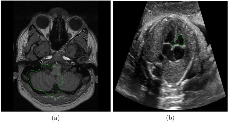
1.1 An MRI slice of an abdominal axial cross sectional view of human body. (a) Example of Region-based segmentation obtained by Kim-mel [67]. (b) Example of Edge-based segmentation obtained by the proposed method in Chapter 3 . The white curves denote the initial contours, the red curves represent the final contour and the green curves represent the ground truth. . . 3

1.2 Examples of gradient kernels along: (a) vertical direction, (b) hori-zontal direction. . . 4

1.3 Pixel aggregation: (a) Image with seeds underlined, (b) segmentation result with τ = 3. . . 5

1.4 Segmentation results on a MRI slice of a spinal cord. (a) Segmen-tation result of image with weak edges. (b) SegmenSegmen-tation result of image with high level of noise. The white curves denote the initial contours, the red curves represent the final contour and the green curves represent the ground truth. . . 8

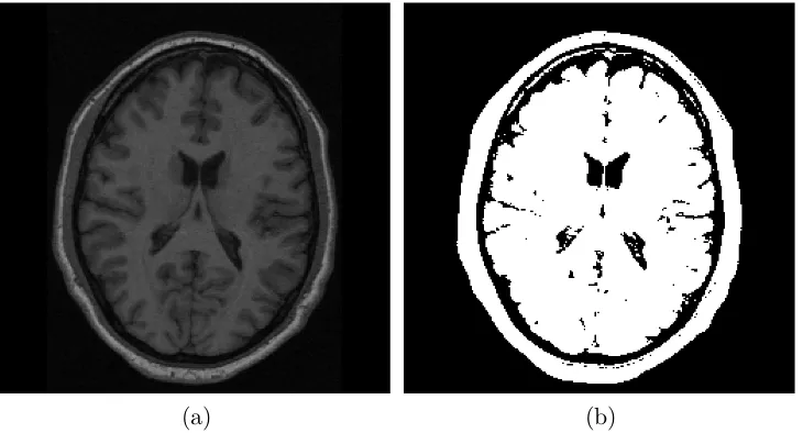
2.1 (a) Templates of a target object in different scales and orientations. (b) Electronic board image where the red box locates the targeted object. . . 15 2.2 (a) MRI image of the brain. (b) The binary segmentation image

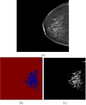
obtained by a thresholding method. . . 16 2.3 (a) A mammogram image of a dense breast. (b) The cluster of

fibrog-landular tissue region obtained by Bayes algorithm. (c) Segmented fibroglandular tissue. . . 17 2.4 Basic form of Snakes. The green dotes represent the snake elements

while the green line represents the contour. . . 23

2.5 : Level set method: (top row) the evolution of the level set function; (bottom row) the evolution of the zero level curve of the corresponding level set function in top row [51]. . . 25 2.6 All possible cases in fitting a curve onto an object. : (a) the curve is

outside of the object; (b) the curve is inside the object; (c) the curve contains both object and background; (d) the curve is on the object boundary [55]. . . 29

3.1 Example of medical image segmentation with weak edges and using GVF active contour. (a) CT slice of skull. (b) 4 Chamber Heart Ultrasound. . . 36 3.2 A GVF snake that fails if initialized by a small curve far from the

desired boundary. The green represents deformation process, white dot represents the manually selected initial position, the red curve represents the initial snake . . . 41

3.5 (a) MR image slice of a human lung, (b) contours or isolines generated from the edge map by PIG [90] . . . 44

3.6 (a),(b) and (c) are the horizontal, vertical and diagonal coefficients, respectively. (d) the edge map. . . 46

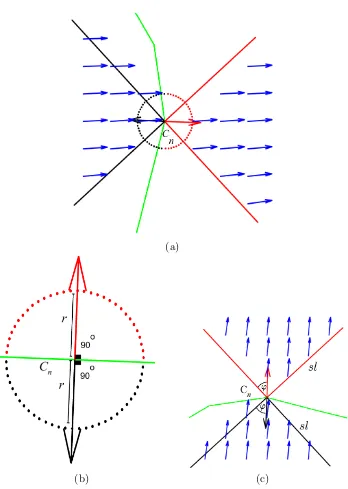
3.7 Region S for snake element Cn. The snake is represented in green.

The red arrow represents the direction of the balloon force which is normal to the snake at elementCn. The blue dotted line represents

regionS of radius r. . . 47

3.8 Region T for snake element Cn. The snake is represented in green.

The red arrow represents the direction of the balloon force, which is normal to the snake at element Cn. Blue arrows represent the GVF

field vectors within regionT. . . 48

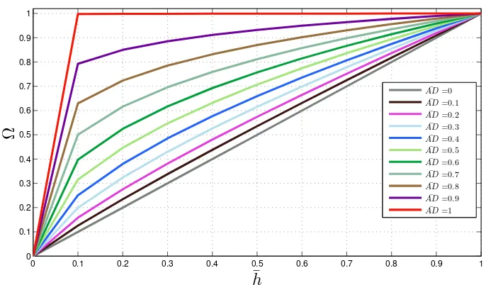
3.9 Value of Ω for different values of ¯h and ¯AD. . . 49

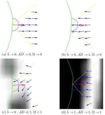
3.10 Direction of the GVF field within region T for different cases where the average amount of edge information (¯h) varies within region S

(the snake is represented in green and non-white pixels represent strong edge information). (a) The direction of the GVF field is similar to the normal direction of growth of the snake (red). (b) The direc-tion of the GVF field is opposite to the normal direcdirec-tion of growth of the snake. (c) The direction of the GVF force field around weak edges. (d) The direction of the GVF force field around strong edges. 50

3.11 (a) RegionsT andS (in red) used to compute Ω, and regionsTb and Sb (in black) used to compute Ωb. (b) Dimension of regionsS and Sb

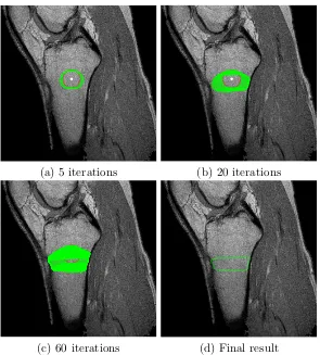
3.12 Final detected boundaries by the GVF snake (yellow), BGrad snake (red), BGVFT snake (blue) and our approach (green). The white dot inside each region represents the manually selected initial position for all evaluated snakes. (a) Image 6 - MRI slice of a knee. (b) Image 1 (upper region) and image 3 (lower region) - an MRI slice of a spinal cord. (c) Image 8 - a CT slice of a skull (left eye). (d) Image 4 (left region) and image 5 (right region)- an MRI slice of a pelvis. . . 55 3.13 Snake deformation process (green curves) for image 2. The white

dot represents the manually selected initial position, the red curve represents the initial snake. . . 59

4.1 The green line represents the evolving contour C, i.e., the zero level setψ(φ,0). The blue lines represent the adjacent contours form= 1,

m=₋1,m= 2 and m=₋2, as specified in Equation (4.11) . . . 69 4.2 The red arrow represents the normal direction of movement of the

evolving contourC. Gray arrows represent the GVF field vectors,V~. The figure shows the case ofk= 2. . . 70 4.3 Value ofω for different values of_I andγ. . . 72 4.4 The normal direction of movement of C for different cases,

4.5 Example of an LSF defined on a grid. The green line represents the evolving contour C, i.e., the zero level set ψ(φ,0). The blue lines represent the contours adjacent to C according to the k value in Equation (4.11); in this figure k= 1. Edge intensity and GVF field values at the the black points along the adjacent contours are used to compute weighting factor ω in Equation (4.10). . . 75

4.6 Boundary detection results of the proposed method on a synthetic im-age with 120 iterations and different values for parameterk. (a)k= 2 (DSC=0.9802). (b) k= 3 (DSC=0.9798). (c) k= 6 (DSC=0.8057). White curves denote the initial contour; red curves denote the final contour, and green curves denotes the ground truth. . . 77

4.7 Different positions for the initial contour on the test synthetic image. 78

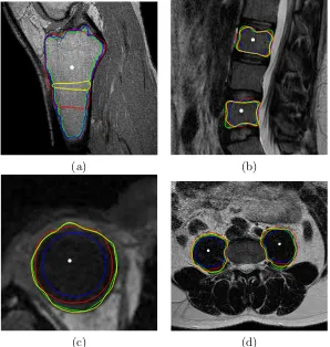
4.8 MRI slice of an abdominal axial cross sectional view of human body. The white curves denote the initial contours, the red curves represent the final contour and the green curves represent the ground truth. . 80

4.9 MRI slice of an abdominal axial cross sectional view of human body. The white curves denote the initial contours, the red curves represent the final contour and the green curves represent the ground truth. . 81

4.11 Visual results for Part 2 experiments. Rows from top correspond to LSD, RD, DRLSE and our proposed method, respectively. The white curves denote the initial contours, the red curves represent the final contour, and the green curves represent the ground truth. For images 27 & 28, the first line of DSC values is for the cecum region (upper region - Experiment 27), while the second line is for the sacrum region (bottom region - Experiment 28). . . 88

4.12 Visual results and DSC values for synthetic images (rows 1 and 2) and real medical images (rows 3 and 4). The first column corresponds to Kimmel’s method, while the second column corresponds to our method. Column 3 depicts a X-ray vessel image, and column 4 depicts an MRI slice of an abdominal axial cross sectional view of the human body. The white curves denote the initial contours, the red curves represent the final contour and the green curves represent the ground truth. . . 89

4.13 Segmentation results on a synthetic image after 100 iterations using different positions for the initial contour. The white curves denote the initial contours, the red curves represent the final contour and the green curves represent the ground truth. Each row shows results for a different initial position. . . 91

4.15 Segmentation results on a MRI slice of a spinal cord (with added noise) after 50 iterations using different positions for the initial con-tour. The white curves denote the initial contours, the red curves represent the final contour and the green curves represent the ground truth. Each row shows results for a different initial position. . . 93

5.1 Examples of overlapping cells with inconsistent staining and poor contrast, which corresponds to a more realistic and challenging setting. 97 5.2 The top row is an overview of the proposed methodology. The

back-ground extraction step aims to separate the clump regions from the background, then to identify the maximum region of each individual cytoplasm within the clump. The cytoplasm segmentation step aims to segment the cytoplsm of each cell within the clump. The bottom row shows example intermediate outputs of the proposed methodol-ogy in a synthetic image depicting overlapping cells. . . 104 5.3 (a) Image generated by MIP. (b) Image generated by EDF. . . 105 5.4 Examples of the original extended depth field (EDF) cervical

cytol-ogy images: (a) typical cervical cytolcytol-ogy image; (b) over-segmented super-pixel map generated by quick shift; (c) binary image represent-ing clump regions. . . 106 5.5 (a) Example of a synthetic cervical cytology image with one clump,

generated by Luet al. [110]. (b) Corresponding labelled image gen-erated by quick shift; the white curve denotes the elliptical shape

Eellipse, and the black curve denotes outer border of regions that

5.6 Examples of the maximum region of overlapping cell in a clump. The green curve denotes the clump region, the red curve denotes the maximum region of the cell, and blue curve denoted the Line. The yellow stars denotesL0 and L1, the possible positions for patch

initialization. . . 110 5.7 (a) Example synthetic overlapping cells; the red contour denotes

over-lapping region, the yellow rectangle denotes patch P0, and the black

rectangles denote the following patches. (b) A close-up view of patch

P0; the orange dotted line denotes the initial open curve, which is

perpendicular to the light blue line connecting c and c0; the green

contour denotes the result of the deformable curve for this patch. . . 111 5.8 Synthetic overlapping cells; the red curve is the detected region of the

cell (Line), and the yellow rectangle denotes the initialized patch, the gray rectangles denote the deformed patch and the green rectangle denotes the last initialized patch. . . 113 5.9 Examples of the original extended depth field (EDF) cervical cytology

images: (a) typical cervical cytology image; (b) nuclei detected by MSER. . . 117 5.10 EDF Cervical Cytology Images. In the first row the curves denotes

the ground-truth and from the secound row to the end the curves denotes the results obtain from each method. . . 120 5.11 Two example of EDF cervical cytology image. Each row represents a

MRI Magnetic Resonance Imaging CT Computed Tomography GVF Gradient Vector Flow PCM Possibilistic C-Means FCM Fuzzy C-Means

CN-GGVF Component-Normalized Generalized-GVF SGVF Sigmoid Gradient Vector Flow

GVC Gradient Vector Convolution PDE Partial Differential Equations PBLS Phase-Based Level Set HAC Harmonic Active Contours LLIF Local Likelihood Image Fitting CoD Centers of Divergence

PIG Poisson Inverse Gradient BGrad Balloon and Image Gradient DSC Dice Similarity Coefficient JC Jaccard Coefficient

DRLSE Distance Regularized Level Set Evolution LSF Level Set Function

SDF Signed Distance Function Pap Papanicolaou

HPVs Human Papillomaviruss

EENCC Edge-Enhancement Nucleus and Cytoplast Contour MSER Maximally Stable Extremal Regions

EDF Extended Depth of Field FOVs Different Fields of View TP True Ppositive

Introduction

The aim of computer vision is to enable computers to see and sense like a human. Research related to computer vision started in 1970s, and it is still being investigated today as a relatively new discipline. Computer vision is considered a branch of arti-ficial intelligence which intends to simulate human behaviour. This gives computer systems the ability to perform functions which normally require human intelligence, such as learning and problem solving. Researchers in the field of artificial intelligence have attempted to integrate computer science and cognitive psychology. Due to the difficulty of integrating human intelligence and cognitive psychology, a computation stream offers an alternative path to more intelligent machine behaviour.

individual objects. Algorithms such as object recognition, segmentation, image cod-ing and robot vision are found on the highest level of the processcod-ing hierarchy. The algorithms used in training a system to recognise or classify an object are considered to be computer vision [1].

The number of publications about computer vision is regularly increasing. In industry, computer vision is frequently used for supporting a manufacturing process, especially in quality control. Other applications of computer vision are, for example, surveillance, image databases, virtual reality, robotics, and security. Perhaps one of the most important uses of computer vision is in medical image analysis. Here the image could be in the form of magnetic resonance imaging (MRI), computed tomography (CT), x-ray, ultrasound images, and so on. This thesis will offer a detailed discussion about the technologies used in image segmentation and with propose novel segmentation methods based on active contours.

1.1

Image Segmentation

Image segmentation is a long standing problem in computer vision. In most image segmentation tasks, individual objects need to be separated from the image. The de-scription of those objects then can be transformed into a form suitable for computer processing. The method of image segmentation is to organise the image content into semantically related groups, which are connected and homogenous according to some properties such as texture, colour and intensity.

(a) (b)

Figure 1.1: An MRI slice of an abdominal axial cross sectional view of human body. (a) Example of Region-based segmentation obtained by Kimmel [67]. (b) Example of Edge-based segmentation obtained by the proposed method in Chapter 3 . The white curves denote the initial contours, the red curves represent the final contour and the green curves represent the ground truth.

1.1.1 Edge-based Segmentation

Edge-based segmentation looks for discontinuities with regard to the intensity of the image. The precise meaning of this process is more edge detection or boundary detection rather than the literal meaning of image segmentation. The boundary between two regions with relatively distinct properties can be defined as an edge. The presumption behind edge-based segmentation is that all sub-regions within a certain image are uniform so that the change between two sub-regions can be determined on the basis of discontinuities alone. Despite this presumption being invalid, region-based segmentation, discussed in the following section, presents more reasonable segmentation results.

Essentially, the concept behind a majority of edge-detection techniques is the computation of a local derivative operator. The gradient vector of an imageI(x, y), given by:

∇I =



 

∂I/∂x

∂I/∂y





where this is obtained by the partial derivatives ∂I/∂x and ∂I/∂x for all pixel locations. The local derivative operation can be performed by convolving an image with kernels, as shown in Figure 1.2.

-1 0 1

(a)

-1 0 1

(b)

Figure 1.2: Examples of gradient kernels along: (a) vertical direction, (b) horizontal direction.

The first derivative magnitude is provided by:

|∇I_|=

q

(∂I/∂x)2+ (∂I/∂y)2. (1.2)

The Laplacian operator of an image functionI(x, y) is the sum of the second-order derivatives, defined as:

∇2I = ∂

2_I

∂2_x + ∂2I

∂2_y. (1.3)

The overall utilisation of the Laplacian operator is in determining the location of edges with the use of zero-crossings [2]. One of the disadvantages of the gradient operation is the noise sensitivity, and as a second-order derivative, the Laplacian operator is even more sensitive to noise. A different option here is to convolve the image with a Laplacian operator of a Gaussian (LoG) function [3]. Thus the two-dimensional Gaussian function can be given by:

G(x, y) = 1

2πσ2exp(−

x2+y2

2σ2 ), (1.4)

whereσ is the standard deviation. The LoG function produces smooth edges as the Gaussian filtering provides a smoothing effect [3].

As a result of its sensitivity to noise, a smoothing operation is usually required as a pre-processing technique to eliminate the noise; consequently, the smoothing effect blurs the edge information. However, the computational cost of the edge detector techniques for edge-based segmentation is relatively low compared to other segmentation methods. This is because the computation can be done by a local filtering operation.

1.1.2 Region-based Segmentation

Region-based segmentation looks for equality inside a sub-region based on a desired property (e.g., colour, texture, and intensity). Clustering techniques, which is based on pattern classification, have similar objectives and can be applied for region-based segmentation. [4].

A technique that is used to merge pixels or small sub-regions into more substantial sub-regions is referred to as region growing [5]. Pixel aggregation, for example, is the simplest implementation of this approach [2]. This approach begins with a series of seed points, and these seed points grow by appending neighbouring pixels if they satisfy the given criteria. An example of pixel aggregation is shown in Figure 1.3.

8 7 2 9 6 1 2 3 4

(a)

8 8 2 8 8 2 2 2 2

(b)

Figure 1.3: Pixel aggregation: (a) Image with seeds underlined, (b) segmentation result withτ = 3.

Segmentation begins with two initial seeds and then the regions grow if they satisfy the criterion:

funda-mental issues exist within region growing. These include selecting the initial seed and relevant properties to grow the regions. The selection of the initial seeds can often be based on the nature of applications or images. For instance, the region of interest is usually brighter than the background. In such a situation, the selection of the brighter pixels as the initial seeds presents the most sensible choice. How-ever, region-based segmentation may produce over-segmented or poor segmentation results.. This mainly due to over-merging the sub-regions with blurry boundaries.

The problem to be solved determines the level of segmentation needed. Usu-ally, the segmentation stops when the region of interest in the application has been detached. As a result of the property of this problem dependence, autonomous segmentation becomes one of the most difficult tasks in image analysis. The seg-mentation problem is even more complicated when the image is subject to noise or poor resolution. Image segmentation can proceed in three different ways:

1. Manual segmentation: This can be done manually by grouping a number

of pixels which shared the same intensity. However, if the image is large, then this task become a very time-consuming method. Alternatively, marking the contours of the objects which can be done from the keyboard or the mouse with higher speed but less accuracy. All manual techniques are time-consuming, and human resources are expensive. Geometrical shapes, like squares or ellipses, are useful to approximate the boundaries of the objects. This has been applied for medical purposes; however, the approximations may not be very good.

2. Automatic segmentation: This refers to the processes whereby segment

3. Semiautomatic segmentation: This combines the advantages of both man-ual and automatic segmentation. By giving some initial information about the structures. This includes, for example, thresholding, clustering and active con-tour methods.

1.2

Medical Image Segmentation

Recent improvements in a wide range of medical imaging technologies have defined anatomical structures and changed how we view the pathological events in the body. Ultrasound X-ray, MRI, nuclear medicine, among other medical imaging technolo-gies captures the structural inside the body in 2D or tomographic 3D images and provide functional information for diagnosis, treatment planning and other purposes. To improve workflow efficiency and to achieve compatibility between imaging sys-tems and other information syssys-tems in healthcare environments a standard called Digital Imaging and Communications in Medicine (DICOM) standard is created as the international standard for communication of biomedical diagnostic and thera-peutic information in disciplines that use digital images and associated data.

The raw form of medical images is represented by arrays of numbers in the computer, where each layer of this array shows different types of body tissue. Pro-cessing and analysis of raw images facilitate the process of extracting meaningful quantitative information to aid diagnosis. Identifies the boundary of objects such as organs or abnormal regions in images is a fundamental problem in medical image analysis. Having segmented organs helps for detecting volume change and shape analysis which it necessary for making a precise therapy treatment plan.

(a) (b)

Figure 1.4: Segmentation results on a MRI slice of a spinal cord. (a) Segmentation result of image with weak edges. (b) Segmentation result of image with high level of noise. The white curves denote the initial contours, the red curves represent the final contour and the green curves represent the ground truth.

medical image segmentation. The active contour model is connectivity-preserving which makes it applicable to the image segmentation problems [6]. Active contours originally proposed by Kass et al. [7] in 1988. Essentially, active contours start with an initial boundary represented in the form of a closed curve. This curve is modified iteratively by inflation or deflation operations according to the application desired. The motion that occurs on the curve by the inflation or the deflation operations is called contour evolution. Those operations are performed by the minimization of an energy function.

1.3 Contributions of Thesis

issues that may hinder the accuracy of any segmentation method formulated using active contour [see Figure 1.4].

1.3

Contributions of Thesis

This thesis proposes novel edge-based active contour methods for medical images that can detect objects’ boundaries even when the background has noise or the object is delimited by a mostly weak boundary. The proposed active contour methods are aimed at providing robust segmentation results for complicated cases with non-uniform backgrounds.

http://www.ijccr.com

VOLUME 1 ISSUE 3 MANUSCRIPT 14 NOVEMBER 2011

particles or objects present in an image. This research paper presents the work to be done on images

having distorted or uneven background and filtering the images to compute statistics of the objects

present in the image. This problem is severe in case of microscopic images captured for the purpose of

bio-medical research where it is difficult to find out the exact shape, size and number of microscopic

particles due to non-uniform illumination and sensitivity to even small fluctuations in light.

Figure 1: Grey-Scale Image showing a cluster of bacteria present in a fluid having non- uniform

texture, brighter on the top and center portions and darker at the bottom.

So, a particular defined area of a photographic plate is taken and exposed by the particles the

characteristics of which are to be computed. The technique used would be to make an algorithm to finally

examine every particle of the image, to see clearly every object in the image, and remove any of the

problems such as non-uniform illumination, less brightness etc. that make it difficult to differentiate

between the particles on the microscopic image shown in figure 1. Various techniques and common

approaches to solve the problem of particle identification are Histogram Equalization, Image Filtering,

Boundary detection, Edge Detection, Linear Filtering, Segmentation, Morphological operations: Dilation

and Erosion etc. But most of these techniques alone fail to accurately determine the objects real

boundaries due to the problem of non-uniform illumination in the background of the image due to which

most of the particles appear to be either dark or light in an image and using techniques such as

histogram equalization, segmentation, edge detection and general image processing algorithms based

on ‘region of interest’ could not differentiate between some of the particles and their background or

http://imsc.uni­graz.at/invcon/medimage/index.html 5/11

     (11)

Here, g is the gyromagnetic ratio of hydrogen, the element in water upon which MRI keys. Also, the gradient pulse G(t) occurs during the pulse sequence interval [0,TE] where TE is the echo time measured in milliseconds. See [Hornak, 1996] for details. Now, because of the symmetry in D, there are seven independent pointwise unknowns among M0 and

D. Therefore, using seven linearly independent gradient fields in successive pulse sequences provides sufficient diffusion­weighted images to permit the diffusion tensor to be determined pointwise.

In particular, imaging the rotational invariants of D has been used to advantage for diagnostic purposes. For instance, the trace of D provides an orientationally averaged apparent diffusivity:

     (12)

and is used to increase lesion conspicuity by suppressing nearby anisotropic effects. On the other hand, when

anisotropic effects are of primary concern, as in the evaluation of nerve fiber tracts, the fractional anisotropy (FA) can be imaged:

     (13)

It is this fractional anisotropy which is mapped in the three images appearing above.

The left­most image shown above is a noisy FA map of the brain, obtained using unfiltered diffusion­weighted images, from which the diffusion tensor images were derived and used in Eqn. (13). The next two images are the results of using the filters discussed in detail earlier for the abdominal MRI. Specifically, the center image shown is the result of applying the Gauss filter to the diffusion tensor images before computing the FA map. As before, note the evident blur in the Gauss filtered image. The right­most image shown is the result of applying the Gauss­TV diffusion filter to the diffusion tensor images before computing the FA map. Again, there is a high contrast level along with a marked reduction in the noise level. See [Keeling, Bammer, Fazekas & Stollberger, 2000].

Restoration of images corrupted by

noise

and

background variations

.

nonuniform background

nonuni uniform background

The purpose of this project is to investigate the enhancement of magnetic resonance images in which broad­band clinical information coexists not only with high gradient noise but also with a slowly varying background variation often seen in MR images. Specifically, this background variation occurs because of the difficulty in generating an ideal, uniform magnetic field for the production of an MR image; see [Hornak, 1996]. For instance, the left image shown above is an MRI of the pelvis. Here, the wide field of view frustrates the task of creating a uniform magnetic field over the entire image region. As a result, the nonuniform background is manifested with the image intensity much higher near the center than toward the periphery. On the other hand, the right image shown is an MRI obtained from an in vitro arthrosclerotic vessel. Here, the field of view is much narrower and there is less difficulty with generating a uniform magnetic field over the sample.

(a) (b)

Figure 1.5: (a) Grey-Scale Image showing a cluster of bacteria present in a fluid having non- uniform texture, darker at the bottom and brighter on the top and center portions. (b) MRI of the pelvis with a slowly varying background variation.

The main contributions are summarised in details as follows:

1. We propose a novel external force, which integrates a gradient vector flow (GVF) field force and a balloon force. This external force is insensitive to snake initialization and may prevent snake leakage. We also propose a mecha-nism to automatically terminate the contour’s deformation. Evaluation results on real MRI and CT slices show that the proposed approach attains higher segmentation accuracy than snakes using traditional external forces, while al-lowing initialization using a limited number of selected points.

2. Motivated by the previous contribution which deforms the contour using a weighting function based on local image features. We propose a level set method for segmentation of medical images with noise and weak edges. The proposed level set evolution is based on the minimization of an objective en-ergy functional whose enen-ergy terms are weighted according to their relative importance in detecting boundaries. This relative importance is computed based on local edge features collected from the adjacent region located inside and outside of the evolving contour. The local edge features employed are the edge intensity and the degree of alignment between the image’s gradient vector flow field and the evolving contour’s normal. Novelties about how local edge information is used in our method are as follows:

(a) Our method measures the alignment between the evolving contour’s nor-mal direction of movement and the image’s gradient in the adjacent region located inside and outside of the evolving contour. This measurement is often used as an additional energy term in the energy functional.

(b) Our method also considers the average edge intensity in the adjacent region located inside and outside of the evolving contour. This allows us to minimize the negative effect of weak edges on the segmentation accuracy.

(c) Our method uses all of the collected local edge information to compute a single value that serves as a weight to control the influence of forces. This minimizes leakage in areas where weak edges exist.

We evaluate the proposed method for segmentation of various regions in real MRI and CT slices, as well as Xray images. Evaluation results show that the proposed method leads to more accurate boundary detection results than other edge-based level set methods, particularly around weak edges.

indi-vidual cell and dealing with the problem of segmenting overlapping cervical cells using edge-based active contours. The main goal of our methodology is to provide significantly fully segmented cells with high accuracy. Due to the chal-lenges involved in delineating cells with severe overlap and poor contrast, most current methods fail to offer a complete segmentation. Although the previous contributions provided promising results in segmenting medical images, how-ever, we can not apply them directly to overlapping cells. Instead, we explore another way of applying edge-based active contour. The proposed framework initially performs a segmentation to cell clumps. Then cell segmentation is performed using a patch-based active contour.

The proposed framework uses a patch-based approach where an active contour detects, on a patch-by-path basis, the cytoplasm boundary of each overlap-ping cell. It also uses a supervised classifier to separate cell clumps from the background and to detect the nuclei of each cell in each clumps. The centriod of each detected nuclei is used to define the major possible region of each cell in the clump. Then, the framework proceeds to allocate the cytoplasm region of each cell. The active contour within the patch is deformed under the influence of GVF forces computed based on local edge features collected from the patch region. Experimental results showed that the proposed frame-work outperforms other state-of-the-art approaches, in terms of segmentation accuracy

1.4

Thesis Outline

The thesis is organized into 6 Chapters. In each chapter, a review of related tech-niques is presented. The individual chapters of this thesis are structured as follows:

• Chapter 3 presents active contours based on weighted gradient vector flow and balloon forces for medical image segmentation. Experimental results are presented and the performance of this method is compared to related states-of-art segmentation algorithms.

• Chapter 4 presents weighted level set evolution based on local edge features for medical image segmentation. Experimental results of this method are presented and the performance of this method is compared to related stats-of-art segmentation algorithms.

• Chapter 5 presents a patch-based segmentation framework for cervical cell images using local information for overlapping cervical cells. Experimental re-sults are presented and the performance of this method is compared to related states-of-art segmentation algorithms.

• Chapter 6 concludes the thesis.

1.5

List of Publications

The list of publication arising from my PhD research on medical image segmentation using edge-based active contours is as follows:

1. A. Khadidos, V. Sanchez and C.-T. Li, “Contours Based on Weighted Gradient Vector Flow and Balloon Forces for Medical Image Segmentation,” in Proc. IEEE International Conference on Image Processing, Paris, France, 27 - 30 Oct 2014.

3. A Khadidos, V. Sanchez, and C-T Li, Weighted Level Set Evolution Based on Local Edge Features for Medical Image Segmentation, IEEE Transactions on Image Processing (accepted and to appear in 2017).

4. A. Khadidos, V. Sanchez and C.-T. Li, “Patch-based Segmentation of Over-lapping Cervical Cells Using Active Contour with Local Edge Information,” in Proc. IEEE International Conference on Acoustics, Speech and Signal Pro-cessing, New Orleans, USA, 5 - 9 March 2017.

The chapters of this thesis are related to the aforementioned papers, as listed in Table 1.1.

Table 1.1: Thesis chapters and the corresponding publications.

Thesis

Chapters Cameras Content

Chapter 3 Paper 1

Contours Based on Weighted Gradient Vector Flow and Balloon Forces for Medical Image Segmentation

Chapter 3 Paper 2 Active Contours with Weighted External Forces for Medical Image Segmentation

Chapter 4 Paper 3 Weighted Level Set Evolution Based on Local Edge Features for Medical Image Segmentation

Chapter 5 Paper 4

Literature Review

2.1

Image Understanding

An image can be represented with a three dimensional matrixw_×h_×n, wherewand

h denote the width and height of an image, andn is the number of channels in an image (i.e., red, green, and blue). In this thesis, the images are represented in grey levels. The total pixel count of an image is defined asw_×h. Image understanding problems are primarily focused on the areas of object detection, segmentation, and class segmentation. A brief summary of these areas is provided in the following subsections.

2.1.1 Object Detection

(a) (b)

Figure 2.1: (a) Templates of a target object in different scales and orientations. (b) Electronic board image where the red box locates the targeted object.

application of the temple matching approach is elementary and straightforward, it proves efficacious for certain applications, it may also be inefficient because of the large size of the search space. Example of template matching algorithm is show in Figure 2.1. Another approach is to select a set of features that are able to differen-tiate the target object and then extract these features from the image and utilise a classifier for the detection stage. Compared to the template matching approach, this process is more robust, although the classifier training process and feature selection are generally required for each new application or dataset [9].

2.1.2 Object Segmentation

a thresholding method is shown in Figure 2.2.

(a) (b)

Figure 2.2: (a) MRI image of the brain. (b) The binary segmentation image obtained by a thresholding method.

The performance of a segmentation algorithm is highly dependent on the feature that is mainly utilised to identify the target object; this is considered ap-plication and data dependent [1]. Object segmentation can be performed in a semi-automated fashion by requesting the user provide the initial labels or fully-automated using pre-trained algorithms that are able to autonomously perform the segmentation [15, 16]. More information is contained in object segmentation than in object detection points, which allow further assessment of object segments. For instance, rather than detecting individuals, human segments permit the recognition of human identity and tracking [17]. Vehicle matching [18] can be implemented rather than estimating the traffic volume and rather than counting the tree crowns, tree crown delineation allows further analysis for species classification [19, 20].

Figure 2.3 shows an image segmented using a Bayes algorithm.

2.1.3 Object Class Segmentation

(a)

50 100 150 200 250

50

100

150

200

250

(b) (c)

Figure 2.3: (a) A mammogram image of a dense breast. (b) The cluster of fibrog-landular tissue region obtained by Bayes algorithm. (c) Segmented fibrogfibrog-landular tissue.

for different datasets.

2.2

Image Segmentation: Methods

Image segmentation has been a well-researched field in the past. Indeed, thousands of segmentation techniques have been proposed so far there, yet there is no a single technique which can be used for any type of images. Therefore, based on the charac-teristics of the image a particular segmentation technique is used [26]. This section briefly reviews the general concepts of existing image segmentation methods.

2.2.1 Clustering

Clustering is the most common form of unsupervised learning, in which classification is done between pixels, and those pixels are grouped to form clusters. Each cluster is a collection of similar pixels, and those that are dissimilar belong to different clusters. The clusters are formed under certain criteria, such as texture, colour, and size. The similarity measure and its implementation play a major role in the quality of the results of the clustering methods.

2.2.2 Region Growing

when deciding to aggregate it. The process of growing reaches the boundary of the region when there is no pixel aggregated, and the growth of the region is going to stop.

2.2.3 Split-and-Merge Algorithms

Unlike the previous method, region merging methods address the problem of image segmentation from the bottom up, where each pixel in the image is considered to be a seed point. In the case of two neighbouring pixels being similar enough according to some criterion, they will merge into a single region. Similarly, if two adjacent regions share the same properties, they will be merged into one region. This process is repeated until merging becomes impossible.

2.2.4 Watershed

The watershed algorithm [28, 29] is a morphology-based segmentation method [30– 32]. The watershed transform is one of popular segmentation methods and was initially proposed by Digabel and Lantuejoul [33]. Watershed transformation meth-ods concede the image as a topographical map with mountains or valleys, where the intensity of a pixel is treated as its altitude. The high-value regions appear as mountains, and the low value regions appears as valleys. The map is then flooded with its local minima. Each water basin fills up from its minima and the dam is formed where two basins converge. Once the water reaches the level of the highest peak, the flooding process is then stopped. The set of all dams defines the so-called watershed.

2.2.5 Graph Partitioning Methods

between pairs of nodes is called weight. To group the pixels, a graph partition is sought to separate the nodes into a disjoint set, so that the similarity among the nodes in the set is high, while the similarity across different sets is low.

2.2.6 Active Contours (Deformable Models)

Deformable models are one of the most used methods in medical image segmentation. A deformable model can be described as a technique for defining region boundaries by using curves or surfaces close to the edges that deform under the effect of forces. Deformable models, including active contours (2-D) and active surfaces (3-D) are closed contours or surfaces which are able to expand or contract over time, within an image, and conform to specific image features [34].There are two main techniques of deformable models in the literature, parametric active contours and geometric active contours. The parametric model represents curves and surfaces explicitly in their parametric forms during deformation. The geometric model is based on the theory of curve evolution in time, according to intrinsic geometric measures of the image, and is numerically implemented via level set algorithms. As image segmentation methods, there are two types of active contour models based on the force that evolves the contours: edge- and region-based. Edge-based active contours, are based on the image gradient, using edge detector output to deform the contour toward the object boundary. This model is closely related to the edge-based segmentation which have been discussed in section 1.1.1. Region-based active contours, instead of searching geometrical boundaries, using statistical information of image intensity within a region.This model is closely related to the region-based segmentation methods which have been discussed in section 1.1.2.

2.2.6.1 Snakes

resembles snake movement. Let us define a contour parameterized by arc length s

as

C(s) ={(x(s), y(s)) : 0≤s≤L}, R→ΩI (2.1)

where L denotes the length of the contour, ΩI denotes the entire domain of an

image I(x, y) and C(s) is a curve sampled and represented by a set of discrete points, these sample points are referred to as snake elements. x(s) and y(s) are a continuous function representing the value of x and y coordinates. Note that the scalar parameter sis between 0 and 1, i.e. the first point in a planar curve is represented asx(0), y(0) , while the last point is represented asx(1), y(1). For closed curves the case is different, the first and last points are the same i.e. x(0) = x(1) andy(0) =y(1).

The main principle behind snakes is to model the movement of a dynamic curve towards an object’s boundary under the influence of internal and external forces. The internal forces depend on the shape of the contour, where the external forces depends on image properties i.e. gradient. An energy functionEsnake(C) can

be defined on the contour such as:

Esnake(C) =Eint+Eext (2.2)

where Eint and Eext respectively denote the internal energy and external energy.

Internal forces control the smoothness of the curve, while external forces lead the curve to the boundary until convergence is achieved.

The internal energy function determines the regularity of the curve. A com-mon choice for the internal energy is a quadratic functional given by:

Eint= 1

Z

0

(α C0(s)

2

+β C00(s)

2

)ds (2.3)

term which controls the contour evolution depending on the imageI(x, y), be defined as:

Eext= 1

Z

0

Eimg(C(s))ds (2.4)

whereEimg(x, y), denotes a scalar function defined on the image plane. Therefore

the image information, such as edges, attracts the snake toward object boundaries. A common example of the edge attraction function is a function of image gradient, given by

f(x, y) =_|∇[Gσ(x, y)∗I(x, y)]|2 (2.5)

whereGσ denotes a 2D Gaussian filter [see Equation 1.4] with standard deviationσ,

∗denotes a linear convolution,∇denotes the gradient operator andI(x, y) denotes the image.

In numerical experiments, a set of snake elements are defined in the initial stage on the image plane and then the next position of those elements is determined by the external energy. The connected elements of a snake are considered as the contour. Basic form of snake is shown in Figure 2.4.

There are number snakes elements in the image, those elements form a con-tour around the object. The snakes elements are initialized at further distance from the boundary of the object. Then, each point moves towards the optimum coor-dinates, where the energy function converges to the minimum. The snake points eventually stop on the boundary of the object.

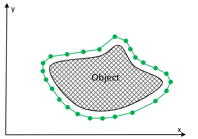
Object

x

y

Figure 2.4: Basic form of Snakes. The green dotes represent the snake elements while the green line represents the contour.

the selection of several initial points or snake elements, which may become a tedious and error-prone process, particularly in medical images.

The classical snake limitations, such as noise sensitivity and initialization sensitivity, motivated other snake variations to be introduced. [36–38], including segmentation of medical images [39–41]. The work of Cohen [37] represents one of the initial solutions, which consists of employing an external force to guide the snake to the object’s boundary in a similar way a balloon inflates or deflates. These

After the introduction of the GVF force, important work has been done to further improve the convergence of snakes. In [35], Zhuet al. propose the gradient and direction vector flow (G&DVF) external force, which integrates the GVF field and prior directional information manually provided by the user. In [43], Qin et al. propose a new external force called the component-normalized generalized-GVF (CN-GGVF), which improves the detection of concave regions and long and thin indentations.

Yao et al. [44] propose the sigmoid gradient vector flow (SGVF) external force, which is obtained by convolving the original image with a sigmoid function before computing the GVF field. This external force, which features a reduced noise sensitivity, is capable of minimizing snake leakages.

Other important solutions that improve convergence of snakes for medical image segmentation include the work in [40, 41]. In [40], Wu et al. propose the gradient vector convolution (GVC) field as an external force, which is calculated by convolving the gradient map of an image with a defined kernel. This method is, however, limited to segmenting specific anatomical regions such as the left ventricle in cardiac MRI. Zhanget al.[41] propose improvements to the GVF snake by using a combination of balloon and tangential forces. This method is, however, very sensitive to a set of parameters.

Figure 2.5: : Level set method: (top row) the evolution of the level set function; (bottom row) the evolution of the zero level curve of the corresponding level set function in top row [51].

context some researchers proposed a deformable surfaces for volume segmentation using an efficient reparameterization mechanism to adopts the topology changes during the curve evolution [46, 47].

2.2.6.2 Level-Set

Despite the excellent performance of snakes, however, it has some intrinsic draw-backs, for example, their limitation to adapt to topological changes, especially if the evolution involves splitting or merging the contour; their inability to detect convex contours; their sensitivity to the initialization position [48]; and their high depen-dency on parametrization. Level set theory has given a solution for this problem [49]. Moreover, it is easy for implementation and lack of parameterization [50].

Osher et al. [49] propose a level set method which implicitly represents the curve as the zero level of the level set φ of a high dimensional function. In parametric active contour models, the contour is represented by a closed planar parametric curve C(s). The curve’s normal is defined by N~ = {−ys(s), xs(s)},

where the subscripts denote derivatives, such that the curve’s tangent is given by

Cs = {xs, ys} = {dx(s)/ds, dy(s)/ds}. The deformable curve may then be

repre-sented implicitly via a two-dimensional φ(x, y) defined on the image plane. The functionφ(x, y) is called level set function or the zero level, of φ(x, y) is defined as the contour, such as

C={(x, y) :φ(x, y) = 0},∀(x, y)∈ΩI (2.6)

where ΩI denotes the entire image plane. Figure 2.5 shows the evolution of a level

set function. While the level set function φ(x, y) deforms from its initial position, the corresponding set of contours propagates outwards. With this definition, the evolution of the contour is equivalent to the evolution of the level set function i.e.

C(s, t) : [0,1]×R2, wheret∈[0,∞) is an artificial time generated by the evolution of the initial curve C0(s) in its inward normal direction N~. For t > 0, the curve’s

evolution equation is given by:

Ct=F ~N (2.7)

whereF is a force function [52]. A formulation of contour evolution using the gradient magnitude ofφ(x, y) was initially proposed by Osher and Sethian [49,53,54], given by

∂φ(x, y)

∂t =|∇φ(x, y)|(F+κ(φ(x, y))) (2.8)

κ=div(∇φ/|∇φ|) (2.9) wherediv(_·) is the divergence operator [50, 52]. The main purpose of the curvature term is to control the regularity of the contours as the internal energy Eint term

does in the classic snakes model.

Another form of contour evolution was proposed by Chan and Vese [55]. The length of the contour|C|can be approximated by a function ofφ(x, y) [56,57], such as

Length_{φ= 0_}=

Z

ΩI

H(φ(x, y))_|∇φ_|dxdy (2.10)

whereH is the Heaviside function.

H(x, y) =

   

  

1, if φ >0 0, if φ_≥0

(2.11)

Since the unit step function produces either 0 or 1 based on on the sign of the input, the derivative of the unit step function produces nonzero only whereφ= 0. As a result, the integration shown in Equation (2.10) is equivalent to the length of contours on the image plane. Parameterizing the descent directions by an artificial timetis given by

∂φ(x, y)

∂t =δ(φ(x, y))k(φ(x, y)) (2.12)

Edge-based Active Contours

Most edge-based active contour models consist of two main terms: the regularity term and edge detection term. The regularity term defines the shape of contours, while the edge detection term attracts the contour towards the edges.

Edge-based active contour model was proposed by Caselleset al.[48] adding an additional term to the speed function shown in Equation (2.8). This term, which added by Caselleset al. , speeds the deformation process of the contour and vanishes when the contour reaches to the object boundary. Similar model proposed by Malladiet al. [50, 58] and is given by

∂φ(x, y)

∂t =g(I(x, y))(κ(φ(x, y) +F)|∇φ(x, y)| (2.13)

whereg_∈[0,1] and it is given by

g, 1

1 +|∇Gσ∗I|2

(2.14)

where ΩI, Gσ is a Gaussian kernel with a standard deviation σ, and ∗ denotes a

convolution operation. Functiongusually takes smaller values at object boundaries than at smooth regions.

The speed of g(I(x, y))(κ(φ(x, y)) +F) moves the contours in the normal direction, and therefore stops on the object boundary, wheregvanishes. The curva-ture termκ maintains the regularity of the contours, while the constant force term

F speed the deformation process and evolve the contour toward the object boundary by minimizing the enclosed area [59].

Region-based Active Contours

and make the models depending on gradients fail to find the contours. The active contours without edges do not depend on the edge of the object. Basically, this model separates the image into regions based on homogeneity of intensities. The

(a)F1(C)>0 (b) F1(C)>0

...F2(C)≈0 ...F2(C)>0

(c) F1(C)≈0 (d) F1(C)≈0

...F2(C)>0 ... F2(C)≈0

Figure 2.6: All possible cases in fitting a curve onto an object. : (a) the curve is outside of the object; (b) the curve is inside the object; (c) the curve contains both object and background; (d) the curve is on the object boundary [55].

region-based active contour models consist of two main terms regularity term and the energy minimization term, which searches for uniformity of a desired feature. The initial contours of region-based active contour can be located anywhere in the image.

Let C be the evolving curve and c1 and c2 two constants, representing the

averages ofu0inside and outside the curveC. Assume thatu0is an image formed by

two regions of approximatively piecewise-constant intensities, with distinct values

ui₀ anduo₀. The object to be segmented is represented by the region with the value

ui₀ whose boundary is denoted by C0. Therefore u0 ≈ c1 inside C and u0 ≈ c2

F1(C) +F2(C) =

Z

inside(C)|

u0−c1| 2

dxdy+

Z

outside(C)|

u0−c2| 2

dxdy (2.15)

If the curveC is outside the object, then F1(C) >0 and F2(C) ≈0. If the

curve is inside the object, thenF1(C)≈0 butF2(C)>0. Finally, the fitting energy

will be minimized if theC =C0 if the curve is on the boundary of the object. This

is illustrated in Figure 2.6.

The energy function with regularizing terms is introduced as follows:

F(C, c1, c2) =µ·length(C) +υ·area(insudeC)

+λ1

Z

inside(C)|

u0−c1| 2

dxdy+λ2

Z

outside(C)|

u0−c2| 2

dxdy (2.16)

where c1 and c2 are constants, and µ > 0, υ ≥0, λ1, λ2 > 0 are fixed parameters.

Thelength and areaterms are regularization terms.

The results obtained by this method partitioned the image which is repre-sented as a set of piecewise-constants, where each subset is reprerepre-sented as a con-stant. This approach has shown the fastest convergence speed in comparison to region-based active contours due to the simple representation.

Level set methods can be categorized into techniques based on partial dif-ferential equations (PDE) [60] or variational level sets [61]. The level set evolution (LSE) of PDE-based methods is mostly based on the geometric considerations of the motion equations [62]. On the other hand, the LSE of variational level set methods is mostly based on optimizing an objective energy functional defined on the level set [61]. Variational level set methods are therefore amenable to incorporating addi-tional information in the LSE, such as region-based information [55,61], shape-prior information [63] and phase-based information [64], which usually gives rise to very accurate boundary detection results.

in-corporate different image features into the energy functional. These methods, which have also been tested on medical images, aim at solving common issues that hinder segmentation accuracy, such as leakage around weak edges and high sensitivity to intensity inhomogeneities [60–62, 64–70]. For example, Kimmel [67] propose an ac-tive contour model with an energy functional that combines an alignment term that leads the curve to the boundary of the desired region. Specifically, the alignment term attempts to align the normal vector of the zero level set with the image’s gra-dient. Although this alignment term leads to more accurate segmentation results, the method may fail to accurately drive the zero level set to the desired boundary around weak edges due to the fact that the gradient of the image around weak edges is relatively small [69].

Belaidet al.[64] propose a phase-based level set (PBLS) method for segmen-tation of medical images with high levels of noise and weak edges. In their approach, the authors construct a speed term based on two phase features: local phase, which is derived from the monogenic signal; and local orientation, which measures the alignment between the local image orientations and the contour’s normal direction of movement. Although PBLS has shown to perform very well in the presence of weak edges, it requires careful tuning of the parameters. [71].

Estellers et al. [69] propose a segmentation method based on the geometric representation of images as 2D manifolds embedded in a higher dimensional space. Their method, termed harmonic active contours (HAC), aligns the image’s gradient with the gradient of the level set function for all the level sets. This results in an objective functional that is able to exploit the alignment of the neighboring level sets to pull the contour to the right position. Although HAC has been shown to provide excellent segmentation results on medical images, it may perform poorly on images with several intensity inhomogeneities [72].

CT images. Based on the image gradient, their method adjusts the effect of the two models. Although this method shows good performance around weak edges, the results are highly dependant on the placement of the initial contour. Ji et al. [74] propose a local region-based active contour model for medical image segmentation that uses the spatially varying mean and variance of local intensities to construct a local likelihood image fitting (LLIF) energy functional. Their method performs well in images with low contrast and intensity inhomogeneities. However, as with other region-based active contour models, it assumes the existence of two well-differentiated regions, which may not always be true in medical images.

2.2.7 Deep Learning Active Contour

Deep learning is a growing trend in data analysis and has been termed recently as one of the breakthrough technologies [75]. Deep learning is a development of artifi-cial neural networks, consisting of more layers that improved predictions from data and allow higher levels of abstraction [76]. Convolutional neural networks (CNNs) shown to be important tools for a broad range of computer vision tasks. Deep CNNs automatically learn high-level and mid-level abstractions obtained from im-ages. Recent studies indicate that the generic descriptors extracted from CNNs are extremely effective in object recognition and localization in medical image analysis especially when applying other deep learning methodologies.

architec-ture, intensity normalization and data augmentation for brain tumour segmentation on MRI. They used a different CNN architectures for low and high-grade tumours. Kallenberget al.[80] proposed unsupervised feature learning for breast density seg-mentation and automatic texture scoring. The model learns features across mul-tiple scales. Once the features are learned, they are fed to a simple classifier that is specific to two different tasks i) breast density segmentation, and ii) scoring of mammographic texture.

Active Contour Based on

Weighted Gradient Vector Flow

and Balloon

3.1

Introduction

Although image segmentation algorithms have been developed over decades it re-mains a complex and challenging task. A given segmentation method may perform well on one problem but it may not work in a different domain. It is very hard to achieve a general segmentation method that is universally applicable for range of different domains.

Deformable models is one of the most used methods in medical image seg-mentation. Deformable model can be described as a technique for defining region boundaries by using curves or surfaces close to the edges that deform under the effect of forces. Deformable models, including active contours (2-D) and active sur-faces (3-D) are closed contours or sursur-faces which are able to expand or contract over time, within an image, and confirms to specific image features [34].

(a) (b)

Figure 3.1: Example of medical image segmentation with weak edges and using GVF active contour. (a) CT slice of skull. (b) 4 Chamber Heart Ultrasound.

of these curves, particularly in medical images as shown in Figure 3.1. In order to overcome these issues, this chapter propose a new external force that combines the advantages of balloon and GVF forces. Specifically, balloon force is employed to guide the snake to the object’s boundary even in the presence of image clutter and noise; while a GVF force is employed to improve convergence to the object’s boundary even around weak edges. The influence of these two types of forces on the snake’s movement is controlled by using a weighting function based on local image features. The proposed external force minimizes snake leakages and considerably reduces the number of initial snake elements, making it suitable for segmentation of medical images with little manual intervention.

3.2

Background

Parametric deformable models represent curves or surfaces in parametric form. The parametric models can be described with two main formulations; formulation of minimizing energy and formulation of dynamic force. The formulation of minimizing energy search for a parametric curve that minimizes a weighted sum of internal energy and external energy. Internal energy controls the smoothness of the curve, while external energy is defined in the image domain and it takes smaller values at smooth regions than object boundaries where the gradient at the edge is high. When internal and external energies are equal, the total energy minimization occurs.

A snake is a curve, first proposed by Kass et al. [7], this curve is sampled and represented by a set of discrete points, these sample points are referred to as snake elements [see Equation (2.1)] . After the curve has been defined, the curve has to be placed near to the boundary of area of interest. Now, a process has to be performed on the curve which makes the curve deform or evolve and this process is called curve evolution [42]. Curve evolution is an iterative computation that makes the curve slide in the selected area on the image. The initialized curve will be pushed by special forces to the object boundary. The curve will stop moving once it reaches the boundary. Based on (2.3) and (2.4) a curve evolves to an object’s boundary by minimizing the following energy function:

ES(C) =

1 2

1

Z

0

(α C0(s)

2

+β C00(s)

2

)ds+

1

Z

0

Eext(C(s))ds (3.1)