Quantitative electrochemical EPR

warwick.ac.uk/lib-publications

A Thesis Submitted for the Degree of PhD at the University of Warwick

Permanent WRAP URL:

http://wrap.warwick.ac.uk/79963

Copyright and reuse:

This thesis is made available online and is protected by original copyright.

Please scroll down to view the document itself.

Please refer to the repository record for this item for information to help you to cite it.

Our policy information is available from the repository home page.

Quantitative electrochemical EPR

By

Mika Tamski

Thesis

Submitted to the University of Warwick

for the degree of

Doctor of Philosophy

Department of Physics

i

List of figures ... v

Acknowledgements ... viii

Declaration and published work ... ix

Abstract ... x

Abbreviations and symbols ... xi

Chapter 1 – Electrochemistry ... 1

1.1. The electrochemical interface ... 1

1.1.1. Structure and dimensions ... 1

1.1.2. Properties ... 3

1.2. The electrochemical setup ... 7

1.3. Electrochemical experiments ... 8

1.3.1. Step methods ... 9

1.3.2. Cyclic voltammetry ... 10

1.4. Mass transport ... 11

1.4.1. Modes of mass transport ... 12

1.5. Ultramicroelectrodes (UMEs) ... 16

1.5.1. Geometry ... 17

1.5.2. Wire electrodes ... 19

References ... 22

Chapter 2 - Electron paramagnetic resonance ... 24

2.1. Uses of EPR... 24

2.2. The Zeeman effect ... 24

2.3. The g-factor ... 28

2.4. Hyperfine interaction ... 30

2.5. EPR spectrometer ... 31

2.6. Microwave power saturation ... 33

ii

2.9. The EPR resonator ... 39

2.9.1. Loop gap resonator (LGR) ... 41

2.9.2. EPR sample classification ... 44

2.9.3. Sensitivity comparison ... 46

2.10. The absolute sensitivity ... 47

References ... 49

Chapter 3 - Electrochemical EPR (EC-EPR) ... 51

3.1. Perturbation functions ... 51

3.2. The motivation for EC-EPR ... 53

3.3. Quantitative EC-EPR (QEC-EPR) ... 56

3.4. Review of EC-EPR cell designs ... 57

3.4.1. Performance criteria and challenges ... 57

3.4.2. Ex situ cells with flow ... 59

3.4.3. In situ cells with flow ... 65

3.4.4. Stationary in situ cells ... 68

References ... 76

Chapter 4 - Quantitative EPR (Q-EPR) ... 80

4.1. The magnetic susceptibility ... 81

4.2. Quantification methods ... 82

4.3. Dielectric properties and resonator Q-value ... 85

4.4. Effective filling factor ... 86

4.5. Magnetic field modulation ... 87

4.6. Microwave power ... 90

4.7. Scan width and double integration ... 92

4.8. Optimising the spectrometer settings ... 95

4.8.1. Setting up phases ... 95

4.8.2. Filter time constant and scan time ... 96

4.9. Referencing ... 97

4.10. What accuracy is achievable ... 97

4.11. Additional challenges due to electrochemistry ... 99

iii

Chapter 5 - The EC-EPR cell and the experimental setup ... 104

5.1. The cell material ... 105

5.2. The cell design ... 106

5.2.1. The first generation EC-EPR cell ... 106

5.2.2. The second generation EC-EPR cell ... 107

5.2.2.1. The cell design ... 107

5.2.2.2. The cell assembly ... 109

5.2.3. The EC-EPR setup ... 111

5.2.4. Benefits of the setup ... 113

5.2.5. Practical advice ... 114

References ... 116

Chapter 6 - The EPR and EC performance of the setup ... 117

6.1. Matherials and methods ... 117

6.2. The EPR performance ... 118

6.2.1. Degassing ... 118

6.2.2. The effect of the sample tube ID towards the EPR performance ... 120

6.2.3. EPR sensitivity comparison between LGR and cylindrical resonator ... 120

6.3. The electrochemical performance ... 123

6.3.1. Finite element simulations ... 123

6.3.2. Experimental results ... 126

6.4. The electrochemical EPR performance ... 129

6.5. Conclusions ... 137

References ... 139

Chapter 7 - Analytical measurements in quantitative EC-EPR ... 140

7.1. Experimental section ... 140

7.1.1. Materials ... 140

7.1.2. Methods ... 141

7.2. Results and discussion ... 142

7.2.1. 1,4-benzoquinone electrochemistry ... 142

iv

7.2.4. SQ-• generation efficiency ... 155

7.3. Conclusions ... 160

References ... 162

Chapter 8 - 1,4-benzoquinone electrochemistry in unbuffered aqueous solutions ... 164

8.1. Background ... 164

8.2. Aims... 173

8.3. Experimental ... 174

8.3.1. Materials ... 174

8.3.2. Methods ... 174

8.4. Results ... 175

8.4.1. Saturation study ... 175

8.4.2. BQ electrochemistry ... 176

8.4.3. pH dependency of radical generation efficiency ... 177

8.4.4. Radical generation efficiency across [BQ] ... 179

8.4.5. Decay kinetics ... 181

8.4.6. Comparison of results ... 186

8.4.7. Spin trapping in BQ solutions ... 187

8.5. Conclusions ... 189

References ... 191

v

Figure 1.1. The electrode-solution interface ... 2

Figure 1.2. A schematic representation of the electric double layer ... 3

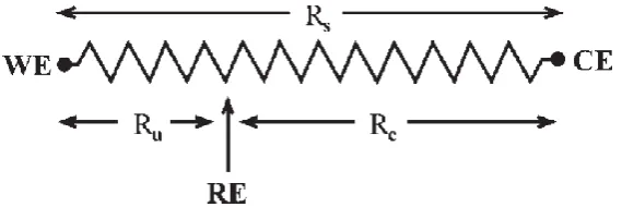
Figure 1.3. Three electrode arrangement for resistance compensation ... 7

Figure 1.4. EC-EPR cell based on flat cell design ... 8

Figure 1.5. A potential step experiment for a reduction of electroactive species ... 9

Figure 1.6. A cyclic voltammetry (CV) experiment for reduction of electroactive species ... 10

Figure 1.7. A concentration profile for [Ox] of the electroanalyte at the WE surface ... 15

Figure 1.8. A diffusion profile for a macro and micro size disc electrodes ... 16

Figure 1.9. Different UME geometries ... 18

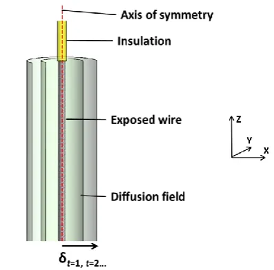
Figure 1.10. Cylindrical geometry with axial symmetry for wire electrode ... 20

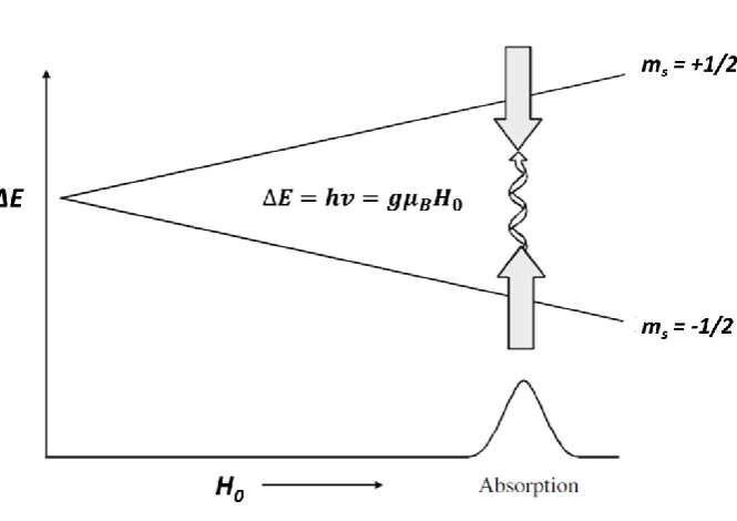
Figure 2.1. The Zeeman Effect ... 27

Figure 2.2. Hyperfine interaction ... 31

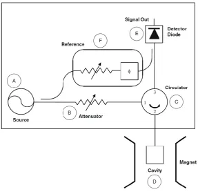
Figure 2.3. The microwave bridge of a CW EPR spectrometer ... 32

Figure 2.4. A schematic representation of the magnetic field modulation ... 34

Figure 2.5. The effect of the width of the absorption line to the height of the line ... 35

Figure 2.6. The effect of increasing radical concentration towards the line broadening ... 38

Figure 2.7. The orientation of electric E1 and magnetic H1 fields in TE102 cavity resonator ... 39

Figure 2.8. One loop two gap resonator ... 42

Figure 2.9. Different LGR topologies ... 43

Figure 2.10. Classification of EPR samples ... 45

Figure 2.11. The sensitivity comparison between one loop one gap LGR and TE102 ... 47

Figure 3.1. The electrochemical interface ... 53

Figure 3.2. The Albery tube electrode ... 60

Figure 3.3. Cylindrical TE011 mode resonator ... 63

Figure 3.4. The schematic representation of the channel electrode cell ... 66

vi

Figure 3.7. Allendoerfer electrochemical cell based on LGR ... 74

Figure 4.1. Frequency dependence of (ε’) and (ε’’) of the dielectric constant of water ... 85

Figure 4.2. Normalised peak-to-peak amplitude (ΔSpp) for first derivatives of Lorenzian and Gaussian lines ... 88

Figure 4.3. Variation of ΔSpp for homogeneously and inhomogeneously broadened lines ... 91

Figure 4.4. The effect of incident microwave power to the double integrated signal intensity of TEMPOL ... 92

Figure 4.5. Double integration ... 93

Figure 4.6. The effect of a finite scan width towards the error related to double integration ... 94

Figure 5.1. 1st generation cell ... 106

Figure 5.2. The cell designed for a LGR ... 108

Figure 5.3. Assembled cell. ... 110

Figure 5.4. A schematic representation of the EC-EPR setup... 113

Figure 6.1. Deoxygenation test ... 119

Figure 6.2. Saturation curves for aqueous 10 μM TEMPOL solution ... 121

Figure 6.3. Comparison of physical sizes ... 122

Figure 6.4. The comparison of aqueous 10 μM TEMPOL EPR spectra ... 122

Figure 6.5. 2D axisymmetric COMSOL model... 124

Figure 6.6. Electrochemical characterization of cells ... 127

Figure 6.7. Cyclic voltammogram for methyl viologen... 129

Figure 6.8. EPR spectrum of MV+• ... 130

Figure 6.9. 5 scan average of EPR transient. ... 131

Figure 6.10. Dynamic EC-EPR ... 133

Figure 6.11. EPR signal intensity vs time for comproportionation ... 135

Figure 6.12. EC-EPR in organic solvent ... 137

Figure 7.1. Saturation curves for (a) TEMPOL and (b) SQ - • ... 141

Figure 7.2. EC-EPR of SQ-• in acetonitrile ... 143

Figure 7.3. The effects of static field in transient measurements ... 145

vii

Figure 7.6. The dependency of the SQ-• centre line width on EPR behaviour ... 150

Figure 7.7. The EPR intensity of H1 and Hmod across the LGR in z-direction ... 154

Figure 7.8. Quantification method ... 156

Figure 7.9. Quantification results ... 157

Figure 7.10. Rate of change of coulombs and EPR SA of a transient ... 159

Figure 8.1. “Nine membered square” for BQ reduction ... 165

Figure 8.2. Possible reduction mechanisms for BQ ... 166

Figure 8.3. Reduction of BQ in unbuffered aqueous solutions ... 167

Figure 8.4. Saturation curve for 100 μM TEMPOL and 1.2 mM BQ ... 175

Figure 8.5. pH dependency of the reduction mechanism of BQ ... 176

Figure 8.6. The pH dependency of radical generation efficiency in 0.9 mM BQ solution ... 178

Figure 8.7. Amount of SQ-• generated vs bulk [BQ] ... 180

Figure 8.8. Decay behaviour of 0.7 mM BQ ... 182

Figure 8.9. The offset relative to the [BQ-•] ... 183

Figure 8.10. An average of 10 transient measurements at 0.1 mM BQ solution ... 183

Figure 8.11. t1/2 vs [BQ] ... 184

viii

ix

I declare that the work presented in this thesis is my own except where stated otherwise, and was carried out at the University of Warwick, during the period of October 2011 and October 2015 under the supervision of Professor M. E. Newton. The research reported here has not been submitted, either wholly or in part, in this or any other academic institution for admission to a higher degree.

Some parts of the work reported and other work not reported in this thesis have been published, as listed below:

Published papers

M. A. Tamski, J. V. Macpherson, P. R. Unwin and M. E. Newton, Physical chemistry chemical physics : PCCP, 2015, 17, 23438-23447.

Conference presentations

I. M. A. Tamski, J. V. Macpherson, P. R. Unwin and M. E. Newton, Loop gap resonators in electrochemical electron paramagnetic resonance, The 6th EFEPR Winter School on Advanced EPR Spectroscopy, Weizmann Institute of Science, Israel, poster presentation (2013)

II. M. A. Tamski, J. V. Macpherson, P. R. Unwin and M. E. Newton, Electrochemical electron paramagnetic resonance utilising microelectrodes and loop gap resonators, The 46th Annual International Meeting of the ESR Spectroscopy Group of the Royal Society of Chemistry, poster presentation (2013)

III. M. A. Tamski, J. V. Macpherson, P. R. Unwin and M. E. Newton, Electrochemical electron paramagnetic resonance utilizing microelectrodes and loop gap resonators,

The 47th Annual International Meeting of the ESR Spectroscopy Group of the Royal Society of Chemistry, University of Dundee, oral presentation (2014)

x

Electron paramagnetic resonance (EPR) is a spectroscopic technique sensitive to unpaired electrons present in paramagnetic species such as free radicals and organometallic complexes.

Electrochemistry (EC) is an interfacial science, where reduction and oxidation processes are studied. A single electron reduction or oxidation generates a paramagnetic species with an unpaired electron, thus making EPR a valuable tool in the study of electrochemical systems.

In this work a novel electrochemical cell was designed and developed to be used with a specific type of EPR resonator, called loop gap resonator (LGR). After building and characterising the performance of the EC-EPR setup, it was adapted for quantitative measurements in electrochemical EPR (QEC-EPR).

xi

Abbreviations

AC Alternating current

AQS Anthraquinonesulfonate

BQ Benzoquinone

CE Counter electrode

CV Cyclic voltammetry

CW Continuous Wave

DC Direct current

DI Double integrated signal intensity of 1st derivative EPR spectrum

DMF Dimethylformamide

DPPH a,a’-diphenyl-β-picrylhydrazyl

EC Electrochemistry

EPR Electron paramagnetic resonance

EC-EPR Electrochemical electron paramagnetic resonance

FcTMA (Ferrocenylmethyl) trimethylammonium hexafluorophosphate

FWHH Full width half height

HOMO Highest occupied molecular orbital

HQ Hydroquinone

LGR Loop gap resonator

LOD Limit of detection

LOQ Limit of quantification

LUMO Lowest unoccupied molecular orbital

MO Molecular orbital

MV Methyl viologen

MW Microwave

NMR Nuclear magnetic resonance

RE Reference electrode

RMS Root mean square

xii WE Working electrode

TBAP tetra-N-butylammonium perchlorate

TEMPAMINE 4-Amino-2,2,6,6-tetramethylpiperidino-1-oxyl

TEMPOL 4-hydroxy-2,2,6,6-tetramethylpiperidin-1-oxyl

TMPD N,N,N’, N’-tetramethyl-para-phenylenediamine

UMEA Ultramicroelectrode array

xiii

a Hyperfine splitting factor

A Electrode surface area

Ap Capacitor plate area

b Band width of the entire detecting and amplifying system

C Concentration

𝐶_𝑗 Concentration of species j

c Resonator conversion factor

Cd Capacitance of the double layer

cr constant from “one time” measurement of a reference standard

ct Filter time constant

𝐶∗ _{Bulk concentration}

𝑑 Distance between capacitor plates

D Diffusion coefficient

𝐷_𝑗 Diffusion coefficient of species j

DO Diffusion coefficient of oxidised form

𝜖 Dielectric constant

εr Relative permittivity of material

E Energy of an electron in an applied field

E1 Electric field of MW irradiation

E Electric potential applied to the electrode

EAppl Applied potential

Eeff Effective potential

EOhm Ohmic drop

Eλ Switching potential

eV Electron volt

ΔE Energy difference of two spin states

ΔE Magnitude of potential perturbation to WE

ΔEp Peak to peak separation

Fn Noise factor for sources other than thermal

F Faraday constant

𝑔 g-factor of a free electron

𝑔𝑒𝑓𝑓 Effective g-factor of a given radical

xiv

ℎ Width of an external magnetic field

ΔHpp peak to peak line width of a 1st derivative EPR line

H0 External magnetic field

Hr Effective magnetic field at resonance

Hmod Modulation amplitude of H0

H1 magnetic field component of the microwave irradiation

HI Magnetic field introduced by a nucleus

i Current

iC Capacitive current

iF Faradaic current

ip Peak current

ipox Anodic peak current

ipred Cathodic peak current

iR Ohmic drop

I Nuclear quantum number

𝐼_𝑠 Steady state current at ultramicroelectrode

𝐽_𝑗 Flux of species j

𝑗_𝑝 Peak current density

kB Boltzmann constant

𝐿 Orbital angular momentum

L Inductance

me Electron mass

ms Spin state of an electron, projection of 𝜇𝑒 in z-direction

n population of an energy state

𝑛 Number of electrons transferred in electrode reaction

𝑛_𝐵 Boltzmann factor for temperature dependence

nS number of scans

Nmin Minimum no. of spins detectable

N Number of spins

NV Sample’s spin volume density

[𝑂]𝑏𝑢𝑙𝑘 Bulk concentration of oxidised form

𝑃_↑ Probability of upward transition

xv

q Charge (in Coulombs)

Q Quality factor of the resonator

QL Loaded Quality factor of the resonator

QU Effective unloaded Quality factor of the resonator

R Universal gas constant

Rc Compensated resistance

Rs Solution resistance

Ru Uncompensated resistance

R Resonator radius

𝑟₀ Radius of cylinder or disc electrode

S Electron spin quantum number

S Width of an experimental scan

ΔSpp peak to peak signal amplitude of a 1st derivative EPR line

t scan time of an EPR spectrum

𝑡 Time (in seconds)

t1/2 Half-life of a radical

tmean Mean lifetime of radical

T Temperature

T1 Spin-lattice relaxation time

T2 Spin-spin relaxation time

Td Detector temperature

Ts Temperature of the sample

v Frequency of the electromagnetic radiation in Hertz

vmod Modulation frequency

𝑣_𝑠 Potential Sweep Rate

𝑣_𝑟𝑒𝑠 Resonator frequency

𝑣_𝑠𝑜𝑙 Velocity of volume element

∆𝑣 Width of the resonator dip at half height

V Signal voltage at the end of the transmission line

Vc Volume of the cavity

Vr Volume of the resonator

Vs Volume of the sample

xvi

Z0 Characteristic impedance of the transmission line

ɀ_𝑗 Electric charge of the species j

𝚲 Resonator efficiency parameter

λ Wavelength of electromagnetic radiation

ƞ Resonator filling factor

τ spin lifetime

𝜏 Cell time constant

Γ line width of the absorption line (half-width half-height)

μB Bohr Magneton

𝜇𝑒 Magnetic moment of a free electron

𝜇𝑁 Nuclear Magnetic Moment

μ0 Magnetic constant (permeability of vacuum)

𝛾𝑒 Gyromagnetic ratio of an isolated electron

𝛿 Diffusion layer thickness

Χ0 Static magnetic susceptibility

Χ’ In-phase component of a dynamic magnetic susceptibility

χ" Out-of-Phase component of the magnetic susceptibility

∅ Electric potential

ω Angular frequency

ε’ Real part of sample’s dielectric constant

1

Chapter 1

– Electrochemistry

Electrochemistry is an old science originating from the work of scientists like Volta and

Galvani, although the utilization of electrochemical phenomena has been traced back to

Parthans (250 B.C.). Modern electrochemistry has develop into a science of interfaces and

has recently been defined as: “Electrochemistry is the study of structures and processes at

the interface between an electronic conductor (the electrode) and the ionic conductor (the

electrolyte) or at the interface between two electrolytes”.1

1.1. The electrochemical interface

At the heart of an electrochemical (EC) experiment is the interface between the electrode

and the sample solution, also called the electric double layer. Several reviews of the electric

double layer have been published in recent years2-4 despite the apparent maturity of the

field. Below the structure and properties of the electrochemical interface are summarised,

before moving on to issues related to mass transport and electrode properties, the main

topics of this chapter.

1.1.1. Structure and dimensions

Although various types electrochemical interfaces exist, the most typical - and relevant to

this thesis - is that between a metallic conductor (electrode) and a solution, the

2

such as salt, acid or base (KCl, HCl, KOH etc.). The interface between the electrode and a

solution acts as a capacitor (Figure 1.1a), where the charge at the metal surface is counter

balanced by ions in the solution. In electrochemical experiments the potential of a working

electrode (WE) and thus the energy of electrons at the metal surface is adjusted with

respect to a reference electrode (RE). When a negative enough potential with respect to

the species of interest (an analyte) is applied to the WE, an electro-reduction of the species

occurs, and an electron is transferred to the lowest unoccupied molecular orbital (LUMO)

(Figure 1.1b). On the other hand, for electro-oxidation, the potential of the WE can be

adjusted to a value positive enough so that an electron is removed from the highest

occupied molecular orbital (HOMO) of the analyte.5

The region across which the charge separation occurs is called the electric double layer, the

structure, dimensions and thus the EC behaviour of which are strongly dependent on the

system under study.6 A schematic representation of the double layer is presented in Figure

1.2, where the net positive charge due to electron deficiency at the metal surface is

confined to an extremely thin layer with a typical thickness of ca. 0.1 Å. At the solution side

3

the equal negative charge is “smeared out” into the solution and thus the potential

gradient across the double layer is more gradual than would be the case with a capacitor

consisting of two parallel metal plates.

The effective dimensions of the double layer are extremely dependent on the system. For

example the concentration and type of the supporting electrolyte affect the distance on

the solution side across which the charge is balanced, ranging from tens of ångstroms in

the case of 0.1 to 1.0 M solutions of strong electrolytes to ca. 100 Å in the case of diluted

systems. None the less, as the voltage applied across the double layer is typically measured

around 1 V, and the separation of the capacitor “plates” is extremely narrow, electric fields

up to 109 V m-1 are realised making the capacitance of the double layer significant.1, 7

1.1.2. Properties

As mentioned above the electric double layer at WE/solution interface, to a good

approximation, acts as a parallel plate capacitor, for which the capacitance can be defined

as:8

Metal (+ve) Solution (-ve)

̴ 0.1 Å 5-20 Å

4 𝐶𝑑=

𝜀𝑟𝐴𝑝

𝑑 , (1.1)

where εr is the relative permittivity of the material between the plates (F m-1) , Ap is the

plate area (m2) and d is the distance between the two plates. The behaviour of the

capacitor can be expressed as:

𝑞

𝐸 = 𝐶𝑑 , (1.2)

where q is the charge stored in the capacitor in Coulombs (C), E is the potential applied

across the capacitor plates in Volts (V) and Cd is the capacitance of the double layer in

Farads (F). When a potential perturbation is applied to the electrode, a current must flow

until the double layer has adjusted to match the new condition of q determined by Cd. It

should be noted that the potential perturbation applied to the electrode introduces

re-distribution of charged particles and solvent dipoles on the solution side, thus effectively

changing the composition and geometry of the other “plate” of the capacitor, and

therefore the capacitance of the electric double layer can be proportional to the applied

potential, unlike in the case of normal capacitors.7 As the potential of the WE is

manipulated during an electrochemical experiment, the charging and discharging of the

capacitor affects the observed signal in the following ways:

 The RC time constant

The magnitude of the charging current is dependent on the resistance of the system, and

5

𝜏 = 𝑅_𝑠𝐶_𝑑 , (1.3)

where τ is the time constant (in seconds) determining the time taken to charge the

capacitor through the solution resistance Rs in Ohms (Ω). For a potential step the behaviour

of the capacitive current (iC) measured in amperes (A), can be expressed as:9

𝑖𝑐=

𝛥𝐸

𝑅𝑠𝑒𝑥𝑝 (−

𝑡

𝑅𝑠𝐶𝑑) , (1.4)

where ΔE is the magnitude of the potential perturbation and t is time (sec). As can be seen,

the iC decays exponentially over time and will distort the analytical Faradaic current (iF), the

recording of which is the aim of EC measurements based on manipulation of the potential.

Therefore a minimum time interval of at least 5τ must be waited for a full establishment of

the potential step, after which the electrochemical interface is charged to a point at which

the desired potential gradient exists at the interface and analytical measurements can be

performed.

Therefore to perform measurements on the shortest timescales possible, the τ should be

minimised. This can be achieved by making the double layer capacitance as small as

possible by minimising the surface area of the WE, and in the case of electrochemical cell

design making sure that the cell geometry does not introduce unnecessary resistance to

the measurements. Because of these requirements it turns out that each individual EC cell

design has a characteristic time constant associated to it, which determines the shortest

6

 The Ohmic Drop (iR-drop)

When current (i) flows during an electrochemical experiment, the measured potential

between WE and RE is distorted due to the Ohmic resistance (EOhm) of the solution:

𝐸𝑂ℎ𝑚= 𝑖𝑅𝑠 , (1.5)

The EOhm term represents the difference between the applied potential (Eappl) and the

effective one (Eeff) established across the electric double layer:9

𝐸_𝑒𝑓𝑓= 𝐸_{𝑎𝑝𝑝𝑙}− 𝐸_{𝑂ℎ𝑚 ,} (1.6)

Where all of the terms can have a time dependency, whether the potential is stepped to a

constant value or swept linearly.

Large currents and solution resistance makes the EOhm more pronounced, and thus

non-polar organic solvents tend to be prone to distorted potential control. Ways to minimise

the effect are to minimise the current by making the WE as small as possible and

decreasing the solution resistance by adding an excess of supporting electrolyte to the

sample solution, which for organic solvents is often not possible due to lack of suitably

soluble supporting electrolytes.7 None the less, the significance of the Rs should not be

ignored, as it contributes to both τ and EOhm.

Decreasing the size of the WE will not only lead to smaller Ohmic drop effect and better

potential control as smaller currents are generated, but also reduce τ due to the smaller Cd.

Therefore the electrochemical performance will improve through the miniaturization of the

7

1.2. The electrochemical setup

So far only a two electrode setup with WE and RE has been considered, which can be

utilised as long as EOhm < 1-2 mV, for example in the case of Rs = 2 kΩ and i = 1 μA (EOhm = 2

mV). In systems where the EOhm due to i, Rs or the cell geometry become significant, a three

electrode configuration can be employed by adding a counter electrode (CE) to the setup.

In this case the current flows between the WE and CE, and the potential of the WE is

controlled relative to the RE. By placing the RE as close to the WE as possible, the overall Rs

can be divided into compensated resistance (Rc) and uncompensated resistance (Ru), thus

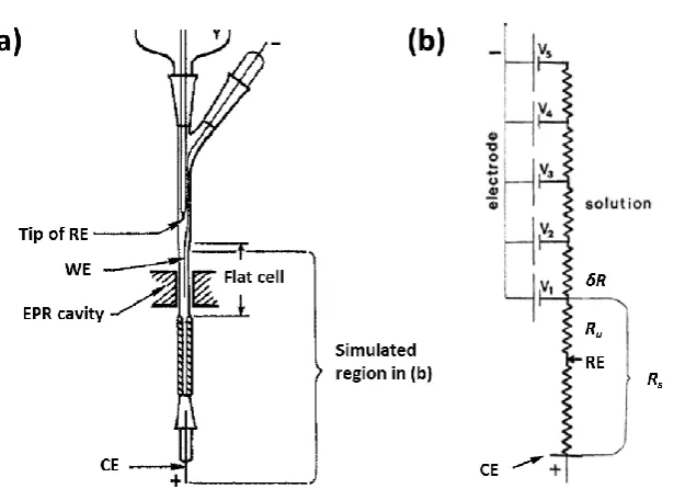
minimising most of the potential drop (Figure 1.3).11

The extent to which a three electrode setup can minimise Ohmic drop depends completely

on the application. For electrochemical EPR, several restrictions in terms of electrochemical

cell geometry, placement of the electrodes and the choice of solvent exist, which affect the

EC performance. For example, in the case of flat cell geometry the current path is limited to

a small cross sectional area making the resistance significant. Furthermore, in a real EC-EPR

cell (Figure 1.4a) the RE is often situated above the WE and the CE below it, making the

Ohmic drop compensation insignificant.

8

Furthermore a second source for the Ohmic drop exists, as the potential across the WE

surface varies depending on the distance from the CE (V1 to V5, Figure 1.4b) especially with

organic solvents, and thus the current density along the WE is not uniform, as it drops in

magnitude moving from segment to segment away from the CE by the amount determined

by δR. Therefore, for large surface area electrodes inside a cell with a small cross section

the placement of the RE close to the WE cannot remove all of the Ru, even if situated

between the WE and CE as shown in Figure 1.4b.12

1.3. Electrochemical experiments

The most common EC techniques utilised with EPR are cyclic voltammetry (CV), potential

steps and current steps, although square wave voltammetry13 and other potential

modulation techniques14 also have been employed.15

9

1.3.1. Step methods

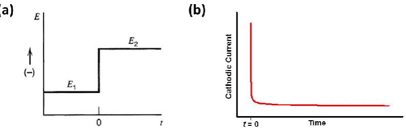
In potential step method (chronoamperometry) the potential of the WE is stepped from an

initial value (E1) where Faradaic processes do not occur to a final potential (E2), where

reduction (or oxidation) of the species of interest does take place (Figure 1.5a). The

corresponding current response is shown in Figure 1.5b for stationary solution, where

diffusion is the only active method of mass transport. After applying the potential E2, the

electrolysis current decays rapidly from the initial high value, as the electroactive species is

depleted from the electrode surface and a relatively slow process of diffusion starts to

transport analyte to the electrode from the bulk solution.5, 16

The Cottrell equation predicts the current behaviour as a function of time in stationary

solutions, where the only mechanism of mass transport is diffusion:

𝑖 =𝑛𝐹𝐴𝐷𝑂

1/2_[𝑂] 𝑏𝑢𝑙𝑘

𝜋1/2_𝑡1/2 , (1.7)

where n is the number of electrons transferred, F is Faraday’s constant, A is the surface

area of the electrode (cm2) , DO is the diffusion coefficient of the electroactive species (cm2

s-1) , [O]bulk is the bulk concentration of the electroactive species (mol cm-3) and t is time

(sec).

Figure 1.5. A potential step experiment for a reduction of electroactive species. (a) The potential of the WE is stepped instantaneously from E1 where no Faradaic current is generated to a value E2 where the analyte is

10

In EC-EPR, potential steps have been used mainly in electrolysis to generate the desired

amount of paramagnetic species for EPR investigation, either to study the EPR spectrum of

the species, or to monitor the EPR signal amplitude as a function of potential and time.17-19

Instead of a potential step, a constant current pulse can be applied, where the WE is set to

deliver a desired current for a specific period of time. In comparison to potential step, this

method allows a better control over the amount of radical species generated for EPR

detection, although decomposition of the solvent can occur if the current pulse is too long,

especially in systems where the Ohmic drop effect is significant.20-23

1.3.2. Cyclic voltammetry

In a cyclic voltammetry (CV) experiment, the potential of the WE is swept linearly from an

initial value to a switching potential (Eλ), where the direction of the sweep is reversed and

scanned back to the original value, as shown in Figure 1.6a. In Figure 1.6b a cathodic

current starts to flow as the potential at the WE reaches a negative enough value for the

reduction to occur. The current increases initially as the electron transfer rate gets faster

with more negative potentials, until a peak value is obtained (ipred), as the diffusion is

Figure 1.6. A cyclic voltammetry (CV) experiment for reduction of electroactive species. (a) The potential of the WE is swept from an initial valuewhere no Faradaic current is generated to a value Eλ, where the sweep

11

unable to supply the WE with fresh analyte at a fast enough rate. During the return sweep

an oxidative peak (ipox) is observed, as the analyte reduced during the first scan is oxidized

back to its original form.5 A voltammetric experiments can also be conducted as a linear

sweep, where only the first potential sweep is applied to the electrode, and thus only the

first current peak recorded.

For large planar electrodes the peak current of the forward scan can be predicted:

𝑖_𝑝= 0.46633/2_𝐴𝐹𝐷

𝑂1/2𝑣𝑠1/2[𝑂]𝑏𝑢𝑙𝑘(

𝐹 𝑅𝑇)

1/2

, (1.8)

where 𝑣𝑠 is the potential sweep rate (V s-1), R is the universal gas constant (J mol-1 K-1) and T

is temperature in Kelvins (K).

In EC the shape and location of the voltammogram on the X-axis can be used to obtain

kinetic and thermodynamic data of the system under study, which in the case of EC-EPR

can then be related to radical generation efficiencies and kinetics of the radical decay.21, 24,

25

1.4. Mass transport

Central to evaluating an EC-EPR cell design and relating the EPR signal behaviour against

processes taking place at the WE surface is the understanding of mass transport

phenomena occurring in electrochemical systems. The electrochemical interface is dynamic

by its very nature, distinguishing it from solid state EPR experiments where the EPR signal

intensity does not change over time due to redistribution of the paramagnetic centres

within the resonator. Below the modes of mass transport are considered, allowing a better

understanding of the EC-EPR technique and challenges towards absolute quantification in

12

1.4.1. Modes of mass transport

Mass transport mechanisms in EC can be divided into diffusion, migration and convection

according to the Nernst-Planck equation, which for a flux in one direction (𝑥) can be

described as:11

𝐽_𝑗(𝑥) = −𝐷𝑗

𝜕𝐶_𝑗(𝑥)

𝜕𝑥 −

ɀ_𝑗𝐹 𝑅𝑇 𝐷𝑗𝐶𝑗

𝜕𝜙(𝑥)

𝜕𝑥 + 𝐶𝑗𝜈𝑠𝑜𝑙(𝑥) , (1.9)

where 𝐽𝑗 is flux of species j (mol cm-2 sec-1) at distance 𝑥 from the electrode surface, 𝐷𝑗

(cm2 sec-1), ɀ𝑗 and 𝐶𝑗 (mol cm-3) are the diffusion coefficient, charge and concentration of

species j, respectively; 𝑣𝑠𝑜𝑙(𝑥) (cm sec-1) is the rate at which a volume element moves in a

solution; 𝜕𝐶𝑗(𝑥) 𝜕𝑥⁄ is the concentration gradient and 𝜕𝜙(𝑥) 𝜕𝑥⁄ is the electric field

gradient along the x-axis.

 Convection

The third term on the right hand side of Equation 1.9 represents the effects of convection.

In EC two types of convection are usually considered. The first type is called natural

convection due to thermal and density gradients that exist within the sample solution.

Natural convection is more typical for macro sized electrodes (mm or more) for

experiments lasting 10-20 sec and more, where the diffusion field starts to collapse

introducing local convective fluxes that are hard to predict or simulate, making analytical

work impossible.

The natural convection can be avoided by introducing a deliberate forced convection to the

EC system, for example by pumping the solution through a channel containing the WE, or

13

through natural convection, allowing the extension of time-scales beyond 10-20 sec. As

long as the hydrodynamic conditions are well defined, it is possible to predict the mass

transport pattern to the electrode surface quantitatively, thus facilitating analytical work.5

As will be discussed in Chapter 3, many EC-EPR cell designs are based on flat cell design,

where natural convection manifests, and thus setups based on forced convection have

been successfully utilised in the study of paramagnetic reaction products.

 Migration

The second term on the right hand side of Equation 1.9 represents the effects of migration.

The 𝜕𝜙 𝜕𝑥⁄ existing at the WE/solution interface will have an electrostatic effect, repulsive

or attractive, to charged species present at the interfacial region, thus introducing a

migratory flux to electrochemical systems. For example, during electrolysis, the

concentration of charged species will change at the electrode surface, affecting the ionic

strength at the interface, and thus the strength of 𝜕𝜙 𝜕𝑥⁄ . Therefore, as the electrolysis

proceeds, the migrational flux and hence the overall mass transport conditions will change

over time, making the system difficult to interpret and quantify.

To avoid migration effects is another reason to add a chemically inert background

electrolyte to the solution. When in large enough excess (typically 100 times relative to the

reactants), the complications due to migration can be avoided, as charge neutrality at the

electrode surface can be assumed and 𝜕𝜙 𝜕𝑥⁄ will not change as the electrolysis proceeds.

As discussed above, the addition of background electrolyte also makes the solution

electrically more conducting diminishing the Ohmic drop effect, ensuring that the current

flowing through the cell during electrolysis is not limited by the conductivity of the bulk

14

 Diffusion

The first term in Equation 1.9 represents Fick’s first law of diffusion, relating flux of species j

to its concentration gradient (how concentration varies over distance 𝑥) at a specific time t.

The second law relates the change in the concentration of species j over time at a given

point:11

𝜕𝐶𝑗

𝜕𝑡 = 𝐷𝑗( 𝜕2_𝐶

𝑗

𝜕𝑥2) , (1.10)

Often the aim of the EC experiment is to make the diffusion the only means of mass

transport. This can be achieved by setting the experiment such that the effects from

convection and migration are negligible by using quiescent solutions, where stirring of the

solution does not occur and adding supporting electrolyte to avoid the migration as

explained above. This greatly simplifies the equation for mass transport (Eq. 1.9), making

the analysis and interpretation of the EC data more feasible.

For simple electrode reactions involving only an electron transfer between the WE and the

species of interest, the Nernst-Planck equation can be used to relate the Eappl to the relative

concentrations of oxidized [Ox] and reduced [Red] species, assuming a reversible system

with fast kinetics so that [Ox] and [Red] are at equilibrium at the electrode surface:11

𝐸_{𝑎𝑝𝑝𝑙} = 𝐸0₊𝑅𝑇

𝑛𝐹𝑙𝑛 [𝑂𝑥]

[𝑅𝑒𝑑] , (1.11)

where E0 is the standard potential. It is assumed that the concentrations of species in

15

Figure 1.7a shows the concentration profile of oxidized species as a function of applied

potential at the WE surface for elementary reduction process according to the

Nernst-Planck equation:

𝑂 + 𝑒−_{⇌ 𝑅 , (1.12)}

where the standard potential for the reduction is -0.2 V. Applying a potential of -0.4 V, for

example, will take the concentration of oxidized species [Ox] to zero at the WE surface,

introducing a concentration gradient between the surface and the bulk of the solution, a

mechanism that establishes the diffusion of more oxidized species towards the electrode.

Whether the potential is swept or stepped to -0.4 V, the concentration gradient will

develop over time getting shallower between the WE surface and the bulk solution [Ox]bulk

as time proceeds and the diffusion layer grows thicker, as shown in Figure 1.7b, where 𝑥 is

the distance from the WE surface. The diffusion layer thickness for linear diffusion can be

estimated from:26

𝛿 = (𝜋𝐷𝑡)1/2 _{, (1.13)}

Figure 1.7. (a) a concentration profile for [Ox] of the electroanalyte at the WE surface as a function of electrode potential according to the Nernst-Planck equation. (b) The growth of the diffusion field and shallowing of the concentration gradient from the WE surface as a function of time for potential where the [Ox] goes to zero. (Modified from ref. [16] pp. 432)

Increasing time

[Ox]_bulk

[Ox]

-0.5 -0.4 -0.3 -0.2 -0.1 0.0 0.1 0.0

0.2 0.4 0.6 0.8 1.0

[Ox]

(mM)

Applied potential (V)

E

16

showing a square root relationship of the diffusion layer thickness with t.

The size of the WE and its geometry will determine the shape of the diffusion field and thus

the magnitude of the diffusive flux to the electrode surface. For example, for a large disk

shaped electrode the diffusive flux is essentially normal or “axial” to the WE surface (Figure

1.8a), whereas for a very small disc (Figure 1.8b) there is a significant radial component to

the diffusion. This results in much increased flux of analyte per unit surface area, giving

small electrodes distinct advantages relative to large electrodes.

1.5. Ultramicroelectrodes (UMEs)

Depending on the geometry of the electrode, the characteristic dimension of a UME should

be around 20 µm at maximum. The benefits of UMEs are:27

I. Small currents are produced, as the electrode is small in size, reducing the

Ohmic-drop as discussed above.

II. The small size of the capacitance and application of smaller over potentials also

decrease the cell time constant. This makes it possible to perform experiments on a

time scale much shorter than with macro electrodes and allows fast-scan

17 voltammetry.

III. The rate of diffusive flux to the electrode increases significantly, and a steady state

concentration of analyte at the electrode surface establishes quickly. The larger

flux of analyte also diminishes the effect of natural convection.

The greatly enhanced mass transport results in high charge densities at the electrode,

producing large Faradaic currents compared to the capacitance and thus high S/N. The

benefits above have enabled electrochemistry to be applied in solid28 and gas phase29, as

well as with non-polar organic solvents without a supporting electrolyte.30

The increased rate of mass transport is caused by the change of the shape of the diffusion

field in the timescale of the experiment.31-33 If the electrode is small enough and of correct

shape, a radial component of the diffusion starts to have a significant effect and the flux of

analyte to the electrode surface is increased. In steady state the rate of reaction is

dependent on electrode kinetics rather than diffusion of the analyte to the electrode

surface, enabling the study of electrode kinetics independently from mass transport. The

exact current response during an experiment is dependent on the geometry of the

electrode via the shape of the diffusion field.34

1.5.1. Geometry

Probably the most common shape of a UME is a disc surrounded by an insulating material

such as glass. A similar geometry is that of a ring, which can be combined with a disc or

rings with different diameter for various applications (Figure 1.9a). Other typical

geometries include those of a cylindrical and a hemispherical, as shown in Figure 1.9b top

and bottom, respectively, and that of a band (Figure 1.9c left). Each of the geometries have

18

homogeneity of the current density across the electrode surface etc. For true steady state

to develop, the electrode geometry must have a convergence factor above 0.5, which is

achieved when the electrode is finite in two dimensions as in the case of a sphere. The

shapes of cylinder and band will not satisfy this requirement being infinite in one

dimension, whereas disc and ring shapes for example can obtain a steady state under

semi-infinite diffusion conditions, as the dimensions are finite provided that the electrode is

small enough.32

Although the very small currents are favourable for electrochemistry, the analytical signal

measured can be of the order of pA or nA, depending on the actual size of the electrode. To

amplify the analytical current, several UMEs can be assembled into an array (UMEA) as

shown for band geometry in Figure 1.9c on the right hand side, which enables the

amplification of the measured signal.35 This increase in the signal is exploited for example in

biosensors36,37, where UMEAs can offer a cheap, fast and reliable method of pesticide and

toxicity testing.38,39

19

1.5.2. Wire electrodes

The electrode geometry relevant to the work in this thesis is the cylindrical one, for which

the Fick’s second law of diffusion, assuming no end effects, can be written as:9

𝜕𝐶 𝜕𝑡 = 𝐷 (

𝜕2_𝐶

𝜕𝑟2 +

1 𝑟

𝜕𝐶

𝜕𝑟) , (1.14)

As seen from equation 1.14, assuming symmetry along the length of the electrode

(z-direction), the diffusion is dependent only on a single dimension (r) in an xy-plane, and

therefore simple to solve mathematically.

Of a cylindrical geometry, metal wire acting as an electrode is one of the simplest and

easiest to manufacture, and the critical dimension characterising the time dependent

behaviour is the radius of the cylinder. Figure 1.10 shows a schematic of a cylindrical wire

electrode, where an axis of symmetry dominates the geometry along the length of the wire

in z-direction, prepared by removing insulation from around a central conductor. Also

shown is the development of the diffusion layer thickness as a function of time, growing

concentrically around the electrode. Over time, the curvature of the diffusion layer

becomes shallower when compared to the curvature at the electrode surface, giving rise to

a radial component to the diffusion, and thus an enhanced flux of analyte to the electrode

surface. None the less, as shown below, it is not possible to obtain true steady state

20

The theory for the diffusion of electro active species to a thin cylindrical electrode has been

developed for potential step42, 43 and linear sweep experiments.40 Provided that the length

of the cylinder is large compared to the radius, the current during a potential step is:

𝑖 =

𝑟0

[

2𝑒𝑥𝑝(−0.05𝜋1/2𝜃1/2)

𝜋1/2_𝜃1/2

+

1

𝑙𝑛(5.2945+0.7493𝜃1/2₎

] ,

with 𝜃 = 4𝐷𝑜𝑡/𝑟02 where r0 is the radius of the cylinder, A the surface area of the electrode

and 𝐶∗ is the bulk concentration (mol cm3). For short timescales 𝜃 is small the current is

essentially Cottrellian, as the first term in the parentheses (Equation 1.15) dominates. The

diffusion remains Cottrellian within 4 % until the diffusion field has become ca. 10 % of r0,

deviating only after the diffusion length becomes large relative to the curvature of the

electrode surface. At this point the radial component of the diffusion causes the current to

increase from that expected for planar macro electrode, as the second term in the

parentheses becomes dominant. Because the current is dependent of time (through 𝜃), no

21

true steady state is ever reached. None the less, as the time manifests only as an inverse

logarithmic function for long time scales, a quasi-steady state is achievable.7

For a linear sweep the empirically obtained peak current density is:

𝑗

=

𝑅𝑇

(

0.446

𝑝

+

0.335

𝑝1.85

)

,

Where 𝑣𝑠 is the scan rate. The value of p characterises the voltammogram, representing

the ratio of the potential scan rate (nF/RT)a𝑣 to the diffusion rate D/a, defined as:

𝑝 = √𝑛𝐹𝑟₀2_𝑣

𝑠/𝑇𝑅𝐷 , (1.17)

For high scan rates or large electrode diameters the values of p are also large, and the

behaviour is similar with linear sweep voltammograms at a large planar electrode, whereas

for very slow scan rates and small electrode diameters the p is small and the behaviour

approaches the steady state solution given by equation 𝐼𝑠= 4𝑛𝐹𝐶∗𝐷𝑟0 for a UME disc.44

None the less, the possibility of adjusting the length of the cylinder allows the utilisation of

currents typical to macro electrodes with some of the benefits of UMEs through radial

22

References

1. E. S. Wolfgang Schmickler, Interfacial Electrochemistry Springer, Heidelberg, London, Germany, 2010.

2. E. Gileadi, J. Solid State Electrochem., 2011, 15, 1359-1371.

3. B. B. Damaskin and O. A. Petrii, J. Solid State Electrochem., 2011, 15, 1317-1334. 4. W. R. Fawcett, J. Solid State Electrochem., 2011, 15, 1347-1358.

5. A. C. Fisher, Electrode Dynamics, Oxford University Press, Oxford, 1996.

6. R. Greef, R. Peat, L. M. Peter, D. Pletcher and J. Robinson, Instrumental Methods in Electrochemistry Ellis Horwood, Chichester, 1985.

7. A. J. Bard and L. R. Faulkner, Electrochemical Methods: Fundamentals and Applications, 2nd edn., JOHN WILEY & SONS, INC., 2001.

8. B. I. Bleaney and B. Bleaney, Electricity and Magnetism, 3rd edn., Oxford University Press, London, 1976.

9. J. Heinze, Angew. Chem. Int. Edit. Engl., 1993, 32, 1268-1288. 10. J. O. Howell and R. M. Wightman, Anal. Chem., 1984, 56, 524-529. 11. M. Ciobanu, J. P. Wilburn, M. L. Krim and D. E. Cliffel, in Handbook of

Electrochemistry, ed. C. G. Zoski, Elsevier, Oxford, UK, 2007, pp. 3-29.

12. I. B. Goldberg, A. J. Bard and S. W. Feldberg, J. Phys.Chem., 1972, 76, 2550-2559. 13. R. D. Allendoerfer, G. A. Martinchek and S. Bruckenstein, Anal.Chem., 1975, 47,

890-894.

14. L. Zhuang and J. T. Lu, J. Electroanal. Chem., 1997, 429, 115-120. 15. R. N. Bagchi, A. M. Bond and F. Scholz, Electroanal., 1989, 1, 1-11.

16. G. Denuault, M. Sosna and K.-J. Williams, in Handbook of Electrochemistry, ed. C. G. Zoski, Elsevier, Amsterdam, Netherlands, 2007, pp. 431-469.

17. R. N. Bagchi, A. M. Bond, F. Scholz and R. Stosser, J. Electroanal. Chem., 1988, 245, 105-112.

18. D. A. Fiedler, M. Koppenol and A. M. Bond, J. Electrochem. Soc., 1995, 142, 862-867.

19. J. G. Gaudiello, P. K. Ghosh and A. J. Bard, J. Am. Chem. Soc., 1985, 107, 3027-3032. 20. R. G. Compton, P. J. Daly, P. R. Unwin and A. M. Waller, J. Electroanal. Chem., 1985,

191, 15-29.

21. I. B. Goldberg and A. J. Bard, J. Phys. Chem., 1971, 75, 3281-3290. 22. I. B. Goldberg and A. J. Bard, J. Phys. Chem., 1974, 78, 290-294.

23. I. B. Goldberg, D. Boyd, R. Hirasawa and A. J. Bard, J. Phys. Chem., 1974, 78, 295-299.

24. W. J. Albery, R. G. Compton and C. C. Jones, J. Am. Chem. Soc., 1984, 106, 469-473. 25. L. Zhuang and J. Lu, Rev. Sci. Instrum., 2000, 71, 4242-4248.

26. C. M. A. Brett and A. M. O. Brett, Electrochemistry: Principles, Methods and Applications, Oxford University Press, Oxford, UK, 1993.

27. S. Pons and M. Fleischmann, Anal. Chem., 1987, 59, A1391-A1399.

23

29. J. Ghoroghchian, F. Sarfarazi, T. Dibble, J. Cassidy, J. J. Smith, A. Russell, G. Dunmore, M. Fleischmann and S. Pons, Anal. Chem., 1986, 58, 2278-2282. 30. A. M. Bond and T. F. Mann, Electrochim. Acta, 1987, 32, 863-870.

31. M. Fleischmann and S. Pons, J. Electroanal. Chem., 1987, 222, 107-115.

32. A. M. Bond, K. B. Oldham and C. G. Zoski, Anal. Chim. Acta, 1989, 216, 177-230. 33. C. G. Zoski, J. Electroanal. Chem., 1990, 296, 317-333.

34. R. M. Wightman, Science, 1988, 240, 415-420.

35. J. Orozco, C. Fernandez-Sanchez and C. Jimenez-Jorquera, Sensors, 10, 475-490. 36. G. A. Evtugyn, H. C. Budnikov and E. B. Nikolskaya, Talanta, 1998, 46, 465-484. 37. M. J. Dennison and A. P. F. Turner, Biotechnol. Adv., 1995, 13, 1-12.

38. D. M. Yong, C. Liu, D. B. Yu and S. J. Dong, Talanta, 2011, 84, 7-12. 39. C. Liu, T. Sun, X. Xu and S. Dong, Anal. Chim. Acta, 2009, 641, 59-63.

40. K. Aoki, K. Honda, K. Tokuda and H. Matsuda, J. Electroanal. Chem., 1985, 182, 267-279.

41. K. Aoki, K. Tokuda and H. Matsuda, J. Electroanal. Chem., 1986, 206, 47-56. 42. K. Aoki, K. Honda, K. Tokuda and H. Matsuda, J. Electroanal. Chem., 1985, 186,

79-86.

43. A. Szabo, D. K. Cope, D. E. Tallman, P. M. Kovach and R. M. Wightman, J. Electroanal. Chem., 1987, 217, 417-423.

24

Chapter 2

- Electron paramagnetic resonance

2.1. Uses of EPR

Electron paramagnetic resonance (EPR) as a technique is sensitive to paramagnetic species

with unpaired electrons only (radical, bi-radical, triplet etc.), and thus provides specific

information on the paramagnetic centre and its environment. Uses of EPR range from the

detection and characterisation of small organic and inorganic radicals in liquids and solids

to organometallic complexes and molecule-based magnetic materials.1

Industrially significant applications of EPR range from polymer formation and degradation

studies2-4 to the food industry, where sterilization through irradiation can be used to

increase hygiene and extend shelf life,5-8 or to measure antioxidant properties of different

foodstuffs.9-11 Other uses of EPR are found from fields such as biology and medicine12, 13,

catalysis14-17 and semiconductor applications.18-21

Below the fundamental theory of continuous wave (CW) EPR is discussed in terms of

phenomena that allow and facilitate the recording of the EPR spectrum.

2.2. The Zeeman effect

A quantum particle such as an electron has an intrinsic spin angular momentum, which is a

vector property having a magnitude and direction. This angular momentum is indicated by

a spin quantum number S and in case of an electron has a value of ½. The electron spin

angular momentum is associated with a magnetic moment μe which for a free electron can

25

𝝁𝒆= −𝑔 𝜇𝐵 𝑺 , (2.1)

where ɡ is the ɡ-factor discussed in a section below with a value of 2.002319 in a vacuum,

µB is the Bohr magneton, a natural unit of an electron’s magnetic moment given by µB =

-|e|h/4πme = -9.27410-24 J T-1, where e is the electron charge, h is the Planck constant

(6.626×10-34 Js) and me is electron mass.

When an external magnetic field (H0 or B0) is applied to an electron spin, the energy is given

as a scalar product between μe and H0:

𝐸 = −𝝁_𝒆∙ 𝑯_𝟎= 𝑔|𝜇_𝐵|𝑺 ∙ 𝑯𝟎 , (2.2)

which assuming that the H0 field orientates along z-direction then becomes:

𝐸 = 𝑔|𝜇_𝐵|𝐻₀𝑆_𝑧 , (2.3)

The projection of μe in z-direction is designated with symbol ms, and for a spin ½ particle

can have only two values: ms= + ½ or ms = – ½, where the negative value represents the

alignment of the magnetic moment along the external magnetic field, and the positive

value against it.

When the external magnetic field is interacting with the electron’s magnetic moment, the

difference in energy (ΔE) between ms = - ½ and ms = + ½ spin states is given by equation:23

26

where Δms has values ±1. ΔE is also the energy required to achieve a transition between

the two spin states. In EPR this energy comes from oscillating magnetic field (H1 or B1) of

microwave (MW) irradiation, where H1 is oriented perpendicular to the H0:

ΔE = ℎ𝜈 = 𝑔 𝜇𝐵𝐻0 , (2.5)

where v is the frequency in Hertz. In a typical EPR experiment at X-band the frequency of

the exciting radiation is around 9.5 GHz. Due to using a resonant cavity coupled to a specific

frequency, it is practical to fix the frequency and sweep the H0 with a laboratory magnet, so

that at resonance the absorption of MW energy occurs according to Equation 2.5 above.

The interaction of the electron magnetic moment with the external magnetic field is called

The Zeeman Effect. When an external magnetic field is applied it introduces a net

magnetization in the sample along the H0 (z-direction), while the components

perpendicular to the H0 (x- and y-directions) are averaged out. In the absence of the

external magnetic field the two mS states are degenerate, i.e. have same energy. Figure 2.1

summarises the interaction between MW irradiation (hν) and μe during an EPR experiment,

when the H0 field is swept and the degeneracy lifted. A resonance condition is achieved

when the energy of the irradiation matches the energy difference between the ms = - ½ and

ms= + ½ spin states.

The population difference Δn of the states can be represented as:24

𝛥𝑛 = 𝑛_−1/2− 𝑛_+1/2 , (2.6)

Where n-1/2 = ½(N + Δn), n+1/2 = ½(N - Δn) and N = n-1/2 + n+1/2. Assuming that spins are

27 𝑑∆𝑛

𝑑𝑡 = −2𝑛−1/2𝑃↑+ 2𝑛1/2𝑃↓ , (2.7)

Where P↑ and P↓ are the probabilities of upward and downward transitions, respectively

and the factor 2 appears because a single transition upwards or downwards changes Δn by

2. It has been shown that in steady state where dΔn/dt = 0:

𝛥𝑛𝑠𝑠_{= 𝑛}

−1/2𝑠𝑠− 𝑛+1/2𝑠𝑠= 𝑁

𝑃↓− 𝑃↑

𝑃_↓+ 𝑃_↑ ,

(2.8)

i.e. population difference exists due to Boltzmann distribution even if the probabilities of

the upward and downward transitions are equal, which can be represented by the

Boltzmann distribution:

Figure 2.1. The Zeeman Effect during an EPR experiment. External magnetic field (H0) is swept while the

microwave radiation (hv) is kept constant. At resonance the energy difference between the spin states match the exciting energy, an absorption of magnetic component of the microwave radiation occurs, and an electron is promoted from parallel ms = - ½ to a higher energy antiparallel ms = + ½ spin state.

28 𝑛_+1/2

𝑛_−1/2= 𝑒

− ∆𝐸_𝑘

𝐵𝑇𝑠 , (2.9)

where n+1/2 and n-1/2 denotes the populations of anti-parallel (ms = +1/2) and parallel (ms =

-1/2) states under thermal equilibrium, respectively, kB is the Boltzmann constant and Ts is

the sample temperature in Kelvins.

Because ΔE is very small, only about 6.2×10-24 J at X-band (H0 = 334 mT, Equation 2.5) and

the thermal energy available at room temperature is relatively large (4.1×10-21 J), the

population difference is only ca. 1/1000 larger for the ms-1/2 state, making net absorption of

energy and thus the EPR signal inherently very weak. An obvious way to increase the signal

intensity is by increasing the population of the ms = -1/2 state relative to ms = +1/2. This can

be accomplished for example by lowering the temperature (Equation 2.9) or increasing the

ΔE by moving to higher frequencies and H0 strengths.22, 23

2.3. The g-factor

In addition to spin angular momentum, an unpaired electron in a molecule also has an

orbital angular momentum associated with it due to the electron’s orbital motion.

Therefore the magnetic moment of a free electron (Equation 2.1) must be modified to

account for this additional source of magnetic moment:22

𝝁 = 𝜇_𝐵(𝑳 + 𝑔𝑒𝑺) , (2.10)

where 𝐿 is the orbital angular momentum, taking integer values depending on the orbital

29

momentum are independent from each other. In practise, although orbital angular

momentum is often quenched and the electron’s angular momentum is only due to its spin,

spin-orbit coupling restores some of the orbital angular momentum, and the g-factor is

adjusted from that of a free electron:

𝑔𝑒𝑓𝑓 =

ℎ𝑣

𝜇_𝐵𝐻_𝑟 , (2.11)

where geff is the effective ɡ-factor accounting for the orbital angular contribution and Hr is

the effective magnetic field at resonance. The geff is unique to any radical species because

the orbital angular momentum of the electron is sensitive to the electron’s surroundings

depending on the molecule in question, and also varies according to which atom the

electron is centred on.

As a result the resonance frequency in Equation 2.5 shifts from that of the free electron to

account for the geff, and therefore the g-factor, in addition to hyperfine couplings discussed

below, can be used as a fingerprint to identify a given molecule. For example an electron in

a vicinity of carbon atom has a ɡ-factor close to the free electron in a vacuum, whereas an

electron close to a heteroatom can have ɡ-factors around 2.004-2.006 and for metal

centres can go up to 9 or 10 in some cases.25

Due to its relation to orbital motion, the spin-orbit coupling is an anisotropic (orientation

dependent) interaction, meaning that the angular momentum varies depending on the

direction of molecular frame relative to H0. This orientation dependency is an important

feature of EPR spectra for single crystal and powder samples in solid form, but also for large

molecules in solvents with high viscosity. For small free radicals in solvents of low viscosity,

ɡ-30

factor anisotropy is averaged out and only the isotropic ɡ-factor needs to be accounted

for.22

2.4. Hyperfine interaction

Certain nuclei such as hydrogen possess a nuclear magnetic moment, μN. The angular

momentum of the unpaired electron spin couples with the magnetic moments of nuclei

present in the molecule, a phenomenon which is called hyperfine interaction. The magnetic

moment of the nucleus induces a small local magnetic field that is experienced by the

unpaired electron and can either enhance or oppose the external magnetic field of the

laboratory magnet. In the simplest case a single hydrogen nucleus with a spin number I = ½

couples with the unpaired electron. Depending on the orientation of the μN of the nucleus,

either more or less external magnetic field is required to introduce the transition between

the electron’s energy state, and therefore two peaks are observed for the electron, one at

lower magnetic field and the other at higher. This is depicted in Figure 2.2, where originally

a single absorption peak is split into two, each centred HI away from the original peak,

where a is the hyperfine coupling factor describing the strength of the interaction between

the electron and nucleus’s magnetic moments.

Depending on the number and nature of the atomic nuclei with I≠0 in the paramagnetic

species, the EPR absorption peak splits in a pattern characteristic to the molecule. This fact

can be used as a fingerprint to identify the radical species and measure the localisation of

the electron spin density within a molecule. As with the ɡ-factor, the hyperfine interaction

displays anisotropy in solids and for large molecules in viscous solvents, but for small free