warwick.ac.uk/lib-publications
Original citation:
Lee, Harim, Moon, Y.-J. and Nakariakov, V. M.. (2015) Radial and azimuthal oscillations of halo coronal mass ejections in the Sun. The Astrophysical Journal, 803 (1). L7.
Permanent WRAP URL:
http://wrap.warwick.ac.uk/78684
Copyright and reuse:
The Warwick Research Archive Portal (WRAP) makes this work by researchers of the University of Warwick available open access under the following conditions. Copyright © and all moral rights to the version of the paper presented here belong to the individual author(s) and/or other copyright owners. To the extent reasonable and practicable the material made available in WRAP has been checked for eligibility before being made available.
Copies of full items can be used for personal research or study, educational, or not-for-profit purposes without prior permission or charge. Provided that the authors, title and full
bibliographic details are credited, a hyperlink and/or URL is given for the original metadata page and the content is not changed in any way.
Publisher’s statement:
Reproduced by permission of the AAS.
Published version: http://dx.doi.org/10.1088/2041-8205/803/1/L7
A note on versions:
The version presented here may differ from the published version or, version of record, if you wish to cite this item you are advised to consult the publisher’s version. Please see the ‘permanent WRAP URL’ above for details on accessing the published version and note that access may require a subscription.
Harim Lee1, Y.-J. Moon1, V. M. Nakariakov1,2
1 School of Space Research, Kyung Hee University, Yongin 446-701, Korea
2 Centre for Fusion, Space & Astrophysics, Physics Department, University of Warwick,
Coventry CV4 7AL, UK
[email protected], [email protected] & [email protected]
ABSTRACT
We present the first observational detection of radial and azimuthal oscil-lations in full halo coronal mass ejections (HCMEs). We analyze nine HCMEs well-observed by the Large Angle and Spectrometric Coronagraph (LASCO) from February to June, 2011. Using the LASCO C3 running difference images, we estimated the instantaneous apparent speeds of the HCMEs in different radial directions from the solar disk center. We find that the development of all these HCMEs is accompanied with quasi-periodic variations of the instantaneous radial velocity with the periods ranging from 24 to 48 minutes. The amplitudes of the instant speed variations reach about a half of the projected speeds. The ampli-tudes are found to anti-correlate with the periods and correlate with the HCME speed, indicating the nonlinear nature of the process. The oscillations have a clear azimuthal structure in the heliocentric polar coordinate system. The oscillations in seven events are found to be associated with distinct azimuthal wave modes with the azimuthal wave number m = 1 for six events and m = 2 for one event. The polarization of the oscillations in these seven HCMEs is broadly consistent with those of their position angles with the mean difference of 42.5 degree. The oscillations may be connected with natural oscillations of the plasmoids around a dynamical equilibrium, or self-oscillatory processes, e.g. the periodic shedding of Alfv´enic vortices. Our results indicate the need for advanced theory of oscillatory processes in CMEs.
1. INTRODUCTION
Coronal mass ejections (CMEs) are the most spectacular eruptions from the Sun into the heliosphere. They are usually main sources of geomagnetic storms (Gosling et al. 1991; Gosling 1993). It has been found that the interplanetary propagation of CMEs is con-trolled by the ambient solar wind (Lindsay et al. 1999; Gopalswamy et al. 2000, 2001a,b; Vrˇsnak & ˇZic 2007). Several authors (Vrˇsnak et al. 2004; Yashiro et al. 2004) suggested that the interaction between CMEs and the solar wind is an important mechanism that deter-mines CME kinematics. One possible mechanism for the deflection of the CME trajectory from radial is the asymmetric aerodynamic drag force associated with formation of Alfv´enic Kelvin-Helmholtz vortices (Foullon et al. 2011).
Dynamical processes in the solar corona are often accompanied by the excitation of various kinds of oscillations of coronal plasma non-uniformities, with the periods ranging from a fraction of a second to several hours. The majority of coronal oscillations have been identified as magnetohydrodynamic (MHD) modes of the non-uniformities (see De Moortel & Nakariakov 2012; Liu & Ofman 2014, for recent comprehensive reviews). The interest in MHD oscillations is connected with a number of open questions, such as heating of the plasma, presence of additional sinks for the energy released in flares, triggering the energy releases, and MHD seismology - diagnostics of plasma parameters and physical processes operating in the plasma by means of MHD oscillations.
It is reasonable to expect that CMEs are accompanied by MHD oscillations that appear naturally as the response of the elastic and compressive plasma to the energy deposition. However, there have been a very few observations of oscillations associated with CMEs. Per-haps the first observation of CME oscillation was reported by Krall et al. (2001). Examining the evolution of the speed pattern of the leading-edge and trailing-edge features for a flux-rope-like CME, they found that the projected CME velocities varied with the period of about 4–6 hr. Shanmugaraju et al. (2010) developed that study, examining the speed-distance pro-files of 116 CMEs with at least 10 height-time data points, and found that about fifteen CMEs had quasi-periodic oscillation patterns. In addition, they showed that the oscillation periods were within the range of the upper and lower limit of the Alfv´en travel time along the magnetic rope of the CME. Very recently, a vertically-polarized kink oscillation with the period of about 11 min was detected in a raising magnetic rope observed in EUV in the low corona (Kim et al. 2014).
2. DATA AND ANALYSIS
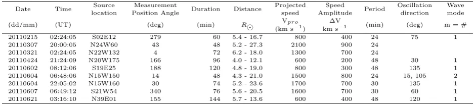
We considered nine well-observed full HCMEs whose structures were clearly seen in the Solar and Heliospheric Observatory (SoHO) Large Angle and Spectrometric Coronagraph’s (LASCO, Brueckner et al. 1995) C2 and C3 fields of view from February to June 2011. These HCMEs were observed at the heights from 4.0 to 27.3 R⊙ with the cadence time about 12–15 minutes. The dates, times, source locations and other properties of the events are summarized in Table 1. In the study we used running difference images obtained from the CDAW LASCO CME online catalogue (http://cdaw.gsfc.nasa.gov/CME list/). Figure 1 shows a typical event analysed in this study, represented by three running difference images taken at different instants of time.
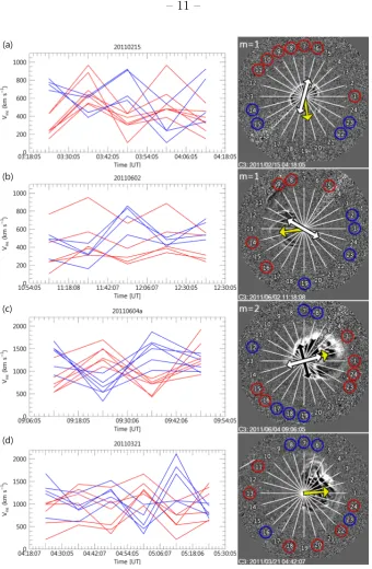
For each available running difference image of the HCMEs we estimated locations of the front edges of the HCME, the outermost and fastest moving structure, at the rays positioned at every 15◦ of the azimuthal angle defined as a counterclockwise from the solar west. These measurements were combined in the height-time maps constructed for different azimuthal angles. The instantaneous speed (Vins) of the HCMEs was determined using two successive height-time measurements at every azimuthal angle for at least four time intervals. Figure 2 shows that the instantaneous speed varies with time (height) quasi-periodically, rather than monotonically increases or decreases.
Parameters of the oscillations we determined by best-fitting the dependence of the in-stantaneous speed upon time by the harmonic function Vins = ∆V sin(ω(t−K)) +b, where
∆V is the amplitude,ω is the cyclic frequency,K is the phase, andbis the mean value, with the use of the least-square method. We also estimated the observed projected speeds (Vpro)
of the HCMEs at every azimuthal angle, which was obtained from a linear fit of height-time data. The results are shown in Table 1.
Some uncertainties in determining the speed of the HCMEs may exist because the determination of the HCME front edge locations are made by the visual inspection. To estimate the uncertainty of the instantaneous speed estimation, we made ten independent trials of the measurements of the front edge locations. Then the error was calculated as its standard deviations for each HCMEs, and the mean value was taken as the measurement. In this study, we estimate the uncertainty of the speed measurement to be about 200 km s−1,
which is an average of the standard deviations. We find that the speed amplitudes ∆V in all the analysed events.
circular shapes. For these cases, the oscillation patterns of these HCMEs at a certain azimuth angle approximately show radial oscillations. To quantify the azimuthal dependence of the oscillatory patterns, we consider the azimuthal dependence in the form of the harmonic function exp(imθ), where θ is the azimuthal angle, and m is an integer representing the azimuthal wave number.
To determine the azimuthal wave number of the oscillations, we applied the following procedure: (1) according to the phase of the oscillations (see the left panels of Fig. 2) we grouped the oscillations detected along individual rays corresponding to different azimuthal angles into “positive” and “negative”; these two groups are shown in the right panels of Fig. 2 by the red and blue circles; (2) we positioned nodal lines between the “red” and “blue” rays; (3) the azimuthal mode number m of the oscillation was obtained as the number of the nodal lines. The polarization of the oscillation was determined in the direction that was perpendicular to the nodal line form= 1, and 45◦ from the nodal line form = 2. The white and black arrows show the directions of the oscillation polarization. The yellow arrows show the HCME position angles (obtained from the LASCO catalogue). We found that the polarization directions are roughly consistent with the HCME position angles with the average discrepancy of 42.5◦.
3. RESULTS
We estimated instantaneous radial speeds of nine full HCMEs at every 15◦ azimuthal angle along 24 rays altogether for each HCME. We found that all the HCMEs had oscillatory patterns in the instantaneous speeds. These oscillatory patterns were found to have opposite phases in different groups of azimuthal directions. As seen in the right panel of Fig. 2, the oscillatory patterns were clearly presented in about 40% of the azimuthal angles. In the left panel of Fig. 2 we give several typical examples of the oscillations. In particular, the 2001 February 15 event (Fig. 2a) is a good example of the m = 1 mode. The observed maximum projected speed and the instantaneous speed oscillation amplitude were found to be about 800 km s−1 and 400 km s−1, respectively. The oscillation period of the HCME is about 24 minutes. The 2011 June 2 event (Fig. 2b) is another case of the m= 1 mode. The observed maximum projected speed and the instantaneous speed amplitude are 800 km s−1 and 300 km s−1, respectively. The oscillation period of the HCME is about 48 minutes. The
2001 June 4 event (Fig. 2c) is a good example of the m= 2 mode. The observed maximum projected speed and the speed amplitude are 1,500 km s−1 and 800 km s−1, respectively. The
panel). The observed maximum projected speed and the speed amplitude are 1,300 km s−1
and 700 km s−1. The oscillation period of the HCME is about 24 minutes.
Figure 3 shows two examples of HCME speed profile (Vins(max)) with the maximum
amplitude and their comparison with the harmonic functions. We find that the observed maximum speeds are approximately fitted by the harmonic functions. The oscillation pa-rameters and the azimuthal mode numbers of all nine events are summarized in Table 1. Durations of the oscillations were found to range from 48 to 144 minutes. The oscillation period ranges from 24 to 48 minutes with the average of 33.3 minutes. In all the events except two the azimuthal wave patterns were found to belong to two lowest azimuthal wave modes, m= 1 in six events and m= 2 in one event.
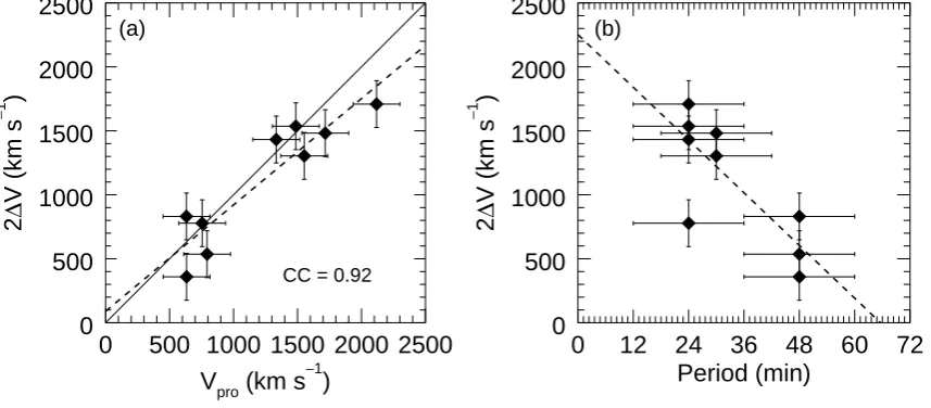
Figure 4a shows a relationship between the oscillation amplitude and maximum pro-jected speed. We found that there is a good correlation, with the correlation coefficient of 0.92, between these two quantities. The speed amplitudes are about a half of the projected speed. Fig. 4b shows a relationship between the speed amplitude and oscillation periods. It is found that the speed amplitude anti-correlates linearly with the period. The oscillation period is thus inversely proportional to the projected speed.
4. SUMMARY AND DISCUSSION
Our study demonstrates the periodic variation of the instantaneous projected radial speed of halo coronal mass ejections. In the lower solar corona, long-period oscillations, with the periods similar to discussed in this Letter, are often detected in prominences (e.g. Bi et al. 2014; Foullon et al. 2009). The oscillations are detected to be either excited by impulsive energy releases (e.g. Hershaw et al. 2011), or result from some over-stabilities processes (e.g. Tripathi et al. 2009). It is not clear whether the HCME oscillations belong to the same class of phenomena. At the coronagraph heights similar oscillations of the radial speed of CMEs have been detected by Krall et al. (2001) and Shanmugaraju et al. (2010). The HCME oscillations discussed here differ from them as we detect the oscillatory motion in the plane perpendicular to the direction of the CME motion. However, if this oscillation is observed from a line-of-sight almost, but not exactly perpendicular to the motion direction, it could result in the variation of the instantaneous radial speed seen by (Krall et al. 2001; Shanmugaraju et al. 2010).
variations of the instantaneous speeds of HCME are found to have a clear structure in the azimuthal direction around the Sun, which corresponds to the “kink” (m = 1) and “fluting” (m= 2) oscillatory patterns. These oscillations could be caused by several physical mechanisms, including natural oscillations, driven oscillations, and self-oscillations.
One interpretation is connected with the natural oscillations of the plasmoid displaced from its equilibrium. In particular, estimations performed by Cargill et al. (1994) and Filippov et al. (2001) showed that a curved magnetic rope could perform oscillations with a period up to several tens of minutes. These models accounted for the restoring force caused by the perturbations of the magnetic field and also the aerodynamic drag force. These results would be consistent with the observed coincidence of them = 1 oscillation polarization with the direction along the HCME position angle. In this case, the observed mode would be the second vertically polarized spatial harmonics (“swaying” oscillations, see D´ıaz et al. 2006) that displaces the CME rope in its plane. The oscillation period of this mode can be estimated as
Pswaying ≈3πDrope/CA, (1)
whereCA is the Alfv´en speed, andDrope is the major diameter of the rope, assuming it has a
circular shape. The rope major diameter can be taken as the HCME diameter divided by 1.5 or so. The factor of 3 accounts for the increase in the period because of effects of curvature and twist (Cargill et al. 1994). From equation (1) we obtained that for the HCME diameter
D = 20R⊙ and the observed periods P = 30 min, the Alfv´en speed should be far too high, about 50,000 km s−1. Even if we neglect the factor of 3, and hence the twist and curvature in
equation (1) the Alfv´en speed is about 16,000 km s−1, which is still unacceptably high. These
values can be reduced by some integer value if we assume that the oscillation corresponds to a higher spatial harmonics along the rope axis, but there is no observational evidence for that. But, it is necessary to stress that the estimation (1) was obtained for a slender rope and it is not clear whether it is applicable to an HCME dynamics. Also, it is not clear whether this model can explain the observed correlation between the oscillation amplitudes and periods and the HCME speed. The established correlation of the oscillation amplitude and the HCME speed is indicative of the nonlinear nature of the observed phenomenon, that needs to be built-in the model.
to shedding of vortices, which is perpendicular to the direction of the motion and hence produces the transverse oscillations, is determined by the flow speed U and the diameterD
of the body, i.e. of the HCME plasmoid, as
Pvort≈(St)−1D/U, (2)
whereStis a dimensionless coefficient known as the Strouhal number. For a bluff sphere, the Strouhal number ranges from 0.2 to 2, see, e.g. Fig. 3 of Sakamoto & Haniu (1990). Making an order of magnitude estimations, we obtain that for the observed period of 30 min, the relative flow speed of 1,000 km s−1 (that can be considered as the difference between the the observed projected speed of the HCME,Vpro, and the solar wind speed), and the HCME diameter of 20R⊙, the Strouhal number should be about 7.7. This value may be acceptable as this estimation is very basic and does not take into account effects of the magnetic field strength and its orientation, and the plasmoid boundary elasticity. Also, the expansion of the CME bubble should possibly lead to the change of the period with time. Perhaps, this effect indeed takes place, but cannot be seen in our data because of the lack of resolution. However, this interpretation should be accepted until detailed theoretical investigation of Alfv´enic vortex shedding by an elastic expanding sphere in a magnetized plasma is carried out.
This work was supported by the BK21 plus program through the National Research Foundation (NRF) funded by the Ministry of Education of Korea, Basic Science Research Program through the NRF funded by the Ministry of Education (NRF-2013R1A1A2012763, 2013R1A1A2058409). VMN acknowledges the support from the European Research Coun-cil under the SeismoSun Research Project No. 321141, and STFC consolidated grant ST/L000733/1. The CME catalog is generated and maintained at the CDAW Data Center by NASA and The Catholic University of America in cooperation with the Naval Research Laboratory. SOHO is a project of international cooperation between the ESA and NASA.
REFERENCES
Aschwanden, M. J., Schrijver, C. J., Winebarger, A.R., & Warren, H. P. 2003, ApJ, 588, L49.
Bi, Y., Jiang, Y., Yang, J., et al. 2014, ApJ, 790, 100
Brueckner, G. E., Howard, R. A., Koomen, M. J., et al. 1995, Sol. Phys., 162, 357
De Moortel, I., & Nakariakov, V. M. 2012, Royal Society of London Philosophical Transac-tions Series A, 370, 3193
D´ıaz, A. J., Zaqarashvili, T., & Roberts, B. 2006, A&A, 455, 709
Filippov, B. P., Gopalswamy, N., & Lozhechkin, A. V. 2001, Sol. Phys., 203, 119
Foullon, C., Verwichte, E., & Nakariakov, V. M. 2009, ApJ, 700, 1658
Foullon, C., Verwichte, E., Nakariakov, V. M., Nykyri, K., & Farrugia, C. J. 2011, ApJ, 729, L8
Gopalswamy, N., Lara, A., Lepping, R. P., et al. 2000, Geophys. Res. Let., 27. 145
Gopalswamy, N., Lara, A., Yashiro, S., Kaiser, M. L., & Howard, R. A., 2001a, J. Geophys. Res., 106, 29207
Gopalswamy, N., Yashiro, S., Kaiser, M. L., Howard, R. A., & Bougeret, J.-L. 2001b, J. Geophys. Res., 106, 29219
Gosling, J. T. 1993, J. Geophys. Res., 98, 18937
Gosling, J. T., McComas, D. J., Phillips, J. L., & Bame, S. J. 1991, J. Geophys. Res., 96, 7831
Gruszecki, M., Nakariakov, V. M., van Doorsselaere, T., & Arber, T. D. 2010, Physical Review Letters, 105, 055004
Hershaw, J., Foullon, C., Nakariakov, V. M., & Verwichte, E. 2011, A&A, 531, AA53
Krall, J., Chen, J., Duffin, R. T., Howard, R. A., & Thompson, B. J. 2001, ApJ, 562, 1045
Kim, S., Nakariakov, V. M., & Cho, K.-S. 2014, ApJ, 797, LL22
Lindsay, G. M., Luhmann, J. G., Russell, C. T., & Gosling, J. T. 1999, Solar Phys., 104, 12515
Liu, W., & Ofman, L. 2014, Sol. Phys., 289, 3233
Nakariakov, V. M., Aschwanden, M. J., & van Doorsselaere, T. 2009, A&A, 502, 661
Sakamoto, H., & Haniu, H. 1990, ASME Transactions Journal of Fluids Engineering, 112, 386
Tripathi, D., Isobe, H., & Jain, R. 2009, Space Science Reviews, 149, 283
Vrˇsnak, B., & ˇZic, T. 2007, Astron. and Astrophys., 472, 937
Vrˇsnak, B., Ruˇzdjak, D., Sudar, D., & Gopalswamy, N. 2004, Astron. and Astrophys., 423, 717
[image:10.595.70.540.265.372.2]Yashiro, S., Gopalswamy, N., Michalek, G., et al. 2004, J. Geophys. Res., 109, 7105
Table 1: List of HCMEs with the oscillation parameters
Date Time Source location
Measurement
Position Angle Duration Distance
Projected speed
Speed
Amplitude Period
Oscillation direction
Wave mode
(dd/mm) (UT) (deg) (min) R⊙ Vpro
(km s−1)
∆V
km s−1 (min) (deg) m = #
20110215 02:24:05 S02E12 279 60 5.4 - 16.7 800 400 24 75 1
20110307 20:00:05 N24W60 43 48 5.2 - 27.3 2100 900 24 20110321 02:24:05 N22W132 4 72 6.2 - 18.0 1300 700 24
20110424 21:24:09 N20W175 166 96 4.0 - 12.1 600 200 48 30 1
20110602 08:12:06 S19E25 188 120 4.8 - 19.0 800 300 48 135 1 20110604 06:48:06 N15W150 14 48 4.3 - 21.0 1500 800 24 15, 105 2 20110604 22:05:02 N15W160 30 74 5.2 - 23.6 1700 700 30 135 1
20110607 06:49:12 S21W54 340 76 5.6 - 20.5 1600 700 30 60 1
20110621 03:16:10 N39E01 155 144 5.7 - 13.6 600 400 48 120 1
Note. — Column 1-2: the first appearance date and time of the HCMEs in the LASCO C2 field of view. Column 3-4: the source location and position angle reported in the CDAW LASCO CME catalogue, respectively. Column 5-6: the duration of the observational interval and the distance range of the HCMEs.
Column 7-8: the maximum projected speed (Vpro), and the maximum oscillation amplitude (∆V). Column
9-11: the period, direction, and azimuthal mode number of the oscillation. If the field is blank, it means a rather complex wave pattern.
Fig. 3.— Two examples of HCME speed profiles Vins(max)(dashed line) with maximum
0 500 1000 1500 2000 2500 Vpro (km s−1)
0 500 1000 1500 2000 2500
2
∆
V (km s
−
1 )
0 12 24 36 48 60 72
Period (min) 0
500 1000 1500 2000 2500
2
∆
V (km s
−
1 )
(a) (b)
[image:14.595.85.514.280.468.2]CC = 0.92