Dynamic adjustment of dispatching rule parameters in flow shops with sequence dependent setup times

warwick.ac.uk/lib-publications

Original citation:

Heger, Jens, Branke, Jürgen, Hildebrandt, Torsten and Scholz-Reiter, Bernd. (2016) Dynamic adjustment of dispatching rule parameters in flow shops with sequence dependent setup times. International Journal of Production Research.

Permanent WRAP URL:

http://wrap.warwick.ac.uk/78472

Copyright and reuse:

The Warwick Research Archive Portal (WRAP) makes this work by researchers of the University of Warwick available open access under the following conditions. Copyright © and all moral rights to the version of the paper presented here belong to the individual author(s) and/or other copyright owners. To the extent reasonable and practicable the material made available in WRAP has been checked for eligibility before being made available.

Copies of full items can be used for personal research or study, educational, or not-for profit purposes without prior permission or charge. Provided that the authors, title and full bibliographic details are credited, a hyperlink and/or URL is given for the original metadata page and the content is not changed in any way.

Publisher’s statement:

“This is an Accepted Manuscript of an article published by Taylor & Francis in International Journal of Production Research on 28/04/2016 available online:

http://www.tandfonline.com/10.1080/00207543.2016.1178406

A note on versions:

The version presented here may differ from the published version or, version of record, if you wish to cite this item you are advised to consult the publisher’s version. Please see the ‘permanent WRAP url’ above for details on accessing the published version and note that access may require a subscription.

Dynamic adjustment of dispatching rule parameters in flow shops with

sequence dependent setup times

Abstract

Decentralized scheduling with dispatching rules is applied in many fields

of production and logistics, especially in highly complex manufacturing

systems. Since dispatching rules are restricted to their local information

horizon, there is no rule that outperforms other rules across various

objectives, scenarios and system conditions. In this paper, we present an

approach to dynamically adjust the parameters of a dispatching rule

depending on the current system conditions. The influence of different

parameter settings of the chosen rule on system performance is estimated

by a machine learning method, whose learning data is generated by

preliminary simulation runs. Using a dynamic flow shop scenario with

sequence dependent setup times, we demonstrate that our approach is

capable of significantly reducing the mean tardiness of jobs.

Keywords: scheduling; simulation; production; artificial intelligence;

flexible manufacturing systems; Gaussian processes

1 Introduction

Many real-world scheduling problems are dynamically changing over time, e.g., due to

new job arrivals, stochastic processing times or machine breakdowns (Aytug et al.,

2005; Oulhadj and Petrovic, 2009). According to the classification of Ouelhadj and

Petrovic (Oulhadj and Petrovic, 2009), there are three categories of dynamic scheduling:

completely reactive, reactive-predictive and robust pro-active scheduling. Dispatching

rules belong to the completely reactive class of scheduling heuristics (e.g., (Haupt 1989;

Blackstone, Philips and Hogg, 1982)) and are widely used to schedule complex shop

floors, e.g., in the field of semiconductor manufacturing (Gupta and Sivakumar, 2006;

Pfund, Mason and Fowler, 2006).

that works best over all scenarios and system conditions. One approach to improve

dispatching rule-based scheduling is thus to switch between dispatching rules

dynamically depending on the current system conditions. Which rule is best for a

particular condition can be determined by simulations? To save simulation time and be

able to handle complex scenarios, machine learning techniques may be applied to

estimate the rule performance and select the best rule (e.g., (Mouelhi-Chibani and

Pierreval, 2010; Heger, Hildebrandt and Scholz-Reiter 2013a; Heger, Hildebrandt and

Scholz-Reiter 2013b). Similarly, the parameters of a compound rule (combining basic

rules) can be set according to the current system conditions. This usually allows more

fine-grained control of rule behavior. In this paper, we present a simulation study of a

flow-shop scenario with sequence-dependent setup times. We have selected the ATCS

(Apparent Tardiness Cost with Setups) (Lee, Bhaskaran and Pinedo, 1997) rule since it

performs well in scenarios with sequence-dependent setup times (Pickardt and Branke,

2011). ATCS is a combination of three different basic rules: WSPT (weighted shortest

processing time), a minimum slack rule as well as the minimum setup time rule. It has

two scaling factors (see equation (1) below), k1 for slack (remaining time until due date

minus remaining processing time) and k2 for setup-avoidance. Setting these parameters

appropriately is crucial for a good performance.

In this paper, we dynamically adjust the k1 and k2 parameters depending on the current

system conditions (e.g., product mix) based on preliminary simulation runs and

performance estimates from Gaussian process (GP) regression models (Williams and

Rasmussen, 1996; Rasmussen and Williams, 2006). In our two-stage approach, we

combine global information based on offline simulation runs with adaptive priority rules

using local information. In contrast to previous work in this area, our approach

considers a truly dynamic scenario, i.e., system conditions are estimated online.

This paper is organized as follows. In Section 2, we give a review of previous research

on dispatching rules especially including setup times and machine learning in

scheduling. In Section 3, our chosen scenario and the experimental design are described.

Section 4 presents the results of our experiments. The paper concludes with a short

2 Problem description and related work

2.1 Scheduling with setup-oriented dispatching rules

Scheduling is “the determination of the order in which a set of jobs (tasks) {i | i = 1, ...,

n) is to be processed through a set of machines (processors, work stations) (k | k=1...m)”

(Haupt, 1989). Most scheduling problems are NP-hard, which means that only very

small problems can be solved optimally in a reasonable time (Monma and Potts, 1989).

But even if realistic static scheduling problems could be solved optimally, in scenarios

with high variability and dynamics, the periodic (re-)calculation of new schedules on a

rolling time horizon would not necessarily lead to overall optimality (Branke, Chick and

Schmidt, 2005). Therefore, in real world settings heuristics are commonly applied.

Heuristics work either in a centralized way (e.g., shifting bottleneck heuristic (Admas,

Balas and Zawack, 1988; Mason, Fowler and Carlye, 2002; Rego and Duarte, 2009)) or

decentralized with decisions made locally regarding the current information available at

the decision point. Decentralized scheduling is applied in scenarios facing high

variability and complexity with continuously arriving new jobs, job changes,

breakdowns, re-entrant processes etc.. Dispatching rules are one class of decentralized

scheduling heuristics (e.g., (Haupt, 1989; Blackstone, Philips and Hogg, 1982)), which

are widely used to schedule complex shop floors. Dispatching rules as a special kind of

priority rules are applied to assign a job to a machine each time the machine becomes

idle and there are jobs waiting. The dispatching rule assigns a priority to each job based

on job, machine or system attributes. The job with the highest priority is chosen to be

processed next.

For scenarios with sequence-dependent setup times, special dispatching rules have been

developed with the objective of avoiding frequent and lengthy changeovers. A recent

overview is given by Pickardt and Branke (2011). Their findings show that the ATCS

rule (Lee, Bhaskaran and Pinedo, 1997) performs well, especially if the objective

function is tardiness related. Mönch, Zimmermann, and Otto (2006) show in their

simulation study of a semiconductor wafer fabrication facility that the total weighted

tardiness and the sum of setup times is sensitive to the k2 setup scaling factor. Chiang

and Fu (2012) proposed the Enhanced Critical Ratio3 (ECR3) rule, which is optimized

for three due date-based objectives. Pfund, Fowler, Gadkari and Chen (2008) suggest

allows non-ready jobs to be scheduled. This means a machine is allowed to stay idle

while waiting for a new job. Van der Zee et al. (2010, 2011 and 2013) have studied the

special case of family based dispatching with batching and sequence-dependent setup

times. Vinod and Sridharan (2009) also study family based dispatching heuristics with

batching. Both results showed that non-exhaustive heuristics can lead to improvements

depending on the system conditions (e.g., utilisation).

2.2 Automatic rule selection / adjustment in static scenarios

Lee and Pinedo (1997) introduced a three-phase heuristic for a problem with one-step

parallel machines and sequence dependent setup times. With four factors describing the

static scenarios, they estimate best values for k1 and k2 of the adapted ATCS rule with a

formula they derived from extensive experiments. The schedule resulting from applying

the dispatching rule is post-processed by a simulated annealing algorithm for

fine-tuning.

Park, Kim, and Lee (2000) extended the approach from Lee and Pinedo (1997) by

adding an additional factor, the setup time range. To determine the scaling parameters k1

and k2 of the ATCS rule, they trained an artificial neural network with five input

parameters and k1 and k2 as outputs with data from preliminary simulation runs of static

scenarios. Their approach was able to outperform the approach introduced by Lee,

Bhaskaran and Pinedo (1997). Another extension has been presented by Chen, Pfund,

and Fowler (2010) who consider the one-stage parallel machine problem with four

characterizing factors as Lee and Pinedo (1997). However, Park, Kim, and Lee (2000)

and Chen, Pfund, and Fowler (2010) only evaluated a one-stage production scenario.

Their approach would need further adaption to be able to continuously estimate the

system parameters and use these to dynamically adapt the ATCS rule.

Mönch, Zimmermann, and Otto (2006) studied a single-stage parallel batch machine

problem with a similar approach. They compared a neural network with an inductive

decision tree to select the k – parameter of the BATC rule, which is an adaption of the ATC rule for batch machines (Balasubramanian, Mönch, Fowler and Pfund 2004). They

considered dynamic job arrivals in their experiments and used system parameters

similar to Lee and Pinedo (1997) and Park, Kim, and Lee (2000). Their results showed

Sequence-dependent setup times were not considered.

Dabbas and Fowler (2003) combine local and global dispatching criteria into a single

rule. A linear combination of rules is combined with relative weights, which are

adjusted regularly dependent on the current WIP.

Pierreval and Mebarki (1997) developed a dispatching approach where the most suited

dispatching rule to the current system state is selected by a new rule. Metan,

Sabuncuoglub, and Pierreval (2010) used a decision tree approach using simulation and

data mining techniques.

2.3. Automatic rule selection / adjustment in dynamic scenarios

As mentioned before, different dispatching rules work well for different settings and

objective functions (Rajendran and Holthaus, 1999; Mouelhi-Chibani and Piereval,

2010). To further improve the performance of rule-based scheduling, the idea of

dynamically switching to the (probably) best rule for the current situation has been

pursued. In most approaches preliminary simulation runs and machine learning

techniques are combined to estimate the performance of candidate rules for the next

decision (Heger, Hildebrandt and Scholz-Reiter, 2013b; Scholz-Reiter, Heger and

Hildebrandt, 2010). A review of machine learning in dynamic scheduling of flexible

manufacturing systems is presented by Priore, de la Fuente, Gomez, and Puente (2010).

Most approaches use artificial neural networks as a machine learning technique.

Sun and Yih (1996) propose a neural network-based controller, which basically selects a

dispatching rule depending on the user’s objective and the current status. The training

samples are calculated by a single-machine simulation and modified to reflect the

impacts of different dispatching rules on the system performance.

Zimmermann and Mönch (2004) present a parameterization scheme of a dispatching

rule to solve a parallel machine batching problem with an inductive decision tree

approach. They adapt the parameter of the BATC rule, which is used for scheduling one

batch machine group.

El-Bouri and Shah (2006) use a neural network to select dispatching rules in a job shop.

that it is limited to scenarios with only a few machines and jobs.

El-Bouri (2012) also introduced a cooperative dispatching approach, which consults

downstream machines before making a decision on the current machine. It basically

represents a look-ahead priority rule-based approach and outperforms standard rules;

however ATC is not considered. His study is performed on a dynamic flow shop

without sequence dependent setup times.

Mouelhi-Chibani and Pierreval (2010) use a neural network to dynamically switch rules

on every machine depending on the current system state. Their scenario consists of only

two machines and the set of dispatching rules consists of the SPT and EDD rule. They

outperform the static use of rules, but not significantly.

Scholz-Reiter et al. and Heger et al. presented the first studies applying Gaussian

processes as a machine learning technique for the selection of dispatching rules

(Scholz-Reiter, Heger and Hildebrandt, 2010; Heger, Hildebrandt and Scholz-(Scholz-Reiter, 2013b).

Gaussian process regression models are used to estimate rule performance in a 10

machine job-shop scenario taken from literature. Preliminary simulation runs are used

to calculate the Gaussian process regression models. They show that these models lead

to better estimates than neural networks in the chosen settings. Mean tardiness can be

improved by more than 6 % in the dynamic scenario.

2.4 Summary of the state-of-the-art

In summary, many different approaches to improve scheduling in a dynamic stochastic

environment have been pursued. First, various priority rules have been proposed, mostly

specialized for particular objective functions or production settings. Nevertheless, due

to the nature of the rules, there is not one best rule for all scenarios, settings and

objective functions. Second, there are studies trying to tackle this drawback by adapting

the rules to the current situation. However, the most relevant studies from Park, Kim,

and Lee (2000) and Mönch, Zimmermann, and Otto (2006) do not consider really

dynamic scenarios simulating the long-term operation of a system, with conditions

changing over time. Mönch, Zimmermann, and Otto (2006) did not study scenarios with

sequence dependent setup times either. The third group of studies investigates neural

study from Mouelhi-Chibani and Pierreval (2010) considers a dynamic scenario, but

only with two machines and no sequence-dependent setup-times.

In our paper, we consider for the first time a complex scheduling problem with setup

times and jobs arriving dynamically over time and an automatic adaptation of the

priority rule parameters.

3 Approach and Experimental setup

The focus of our work is to develop a new scheduling method for manufacturing

scenarios with sequence-dependent setup times, which automatically adjusts to the

current system conditions (e.g., product mix). To this end, we suggest performing

preliminary static simulation runs in an offline phase to investigate which parameter

setting works best for each system state. Since there are many possible combinations

and simulation runs can be computationally expensive, we use Gaussian process

regression models to estimate the performance of unknown parameter settings. In the

application phase, these Gaussian process models are used for the dynamic setting of

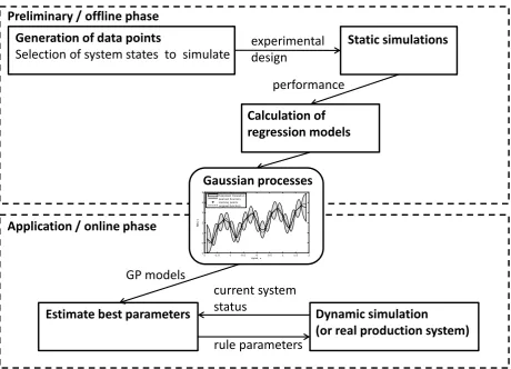
the rule parameters depending on the current system situation. An overview of the

Figure 1. Overview of the dynamic adjustment approach

3.1 Scenario description

The type of problems we address are shop scenarios with new jobs arriving dynamically

over time. Our computational experiments used to demonstrate the advantages of our

approach are based on a dynamic flow-shop scenario, which extends the flow-shop

scenario from Rajendran and Holthaus (1999). In total there are 10 machines on the

shop floor, each job has the same route, i.e., machine visitation order is strict, and there

are no re-entrant flows. Processing times are drawn from a uniform discrete distribution

ranging from 1 to 49 minutes. The due dates of the jobs are determined by a due date

tightness factor x, a job’s due date is set to x times the job’s total processing time +

release time. Job arrival is a Poisson process, i.e., inter-arrival times of jobs follow an

exponential distribution. The arrival rate is set to yield a desired long term utilization

level on each machine. We consider three product types with the setup matrix for each

machine shown in figure 2.

Generation of data points

Selection of system states to simulate experimental_design Static simulations

performance Preliminary / offline phase

Calculation of regression models

Estimate best parameters Application / online phase

Dynamic simulation

(or real production system) current system

status

rule parameters -2 -1.5 -1 -0.5 0 0.5 1 1.5 2 -1

0 1 2 3 4 5

input, x

input

, y

Standard Deviation learned function training points original function

Gaussian processes

0 10 25 5 0 25

5 10 0

 

 

 

 

 

Figure 2. Setup matrix for 3 families

The considered objective function is mean tardiness. However, it should be

straightforward to extend the approach to other objectives.

3.2 Dispatching rules

The idea of our approach is to choose the best dispatching rule for the current system

condition. If, for example, a machine is highly utilized, a rule avoiding setups is

preferable. In low utilization, selecting the most urgent jobs should lead to a lower mean

tardiness. To achieve this, we need to use different dispatching rules for different

situations. As an alternative to switching rules, we can use composite rules that have an

integrated term for setup avoidance. These are usually based on common dispatching

rules that have proven to be effective on flow time- or tardiness-related performance

criteria (Pickardt and Branke, 2011). The ATCS rule is one of the most effective rules

with respect to mean tardiness and considers the slack (time until due date minus

remaining processing time of the job) and the setup avoidance separately. Two scaling

parameters (k₁, k₂) are used to tune the weights given to certain rule components. The

priority index of job j is calculated by the following formula

(

)

1 2

max ,0

: j exp j j exp ij

j j

d p t

w s

ATCS

p k p k s

  − −     = _− _{ }− _    

, (1)

where w_j is the weight of job

j

time, t the time of decision-making, p the average processing time of the jobs, s the average setup time of the jobs, k₁ the scaling factor for slack and k₂ the scaling factor

for setup time. The job with the highest priority value is chosen. Choosing the right

values for k₁ and k₂ is crucial for good performance (Mönch, 2007). Usually these

scaling factors are kept constant for a given scenario. Since most real life scenarios are

parameter on every machine is investigated in this paper. There are no urgent jobs

considered, so the weight of all jobs is set to 1.

3.3 Machine learning

Machine learning is a branch of artificial intelligence which tries to derive patterns or

predictions from a given dataset, usually called the training data. We are interested in a

system which can predict the value of an objective function (i.e., mean tardiness)

depending on the system characteristics and parameter settings of the control rule. This

allows to predict the best parameter setting depending on the system characteristics.

Training data is gained by surveying past production processes or performing

simulation runs. As inputs we have system attributes (e.g., product mix etc.) and

parameter settings (e.g., values for k₁ and k₂) affecting the output (e.g., mean

tardiness).

For our experiments we have chosen Gaussian process regression models (Rasmussen

and Williams, 2006) since studies from Rasmussen and Williams (1996), Scholz-Reiter,

Heger, Hildebrandt (2010) and Heger, Bani, and Scholz-Reiter (2012) showed that they

outperform other techniques in similar settings. Gaussian processes are relatively easy

to set up. To learn the performance models the Gaussian processes require some

training data as well as a covariance function. This covariance function, sometimes

called kernel, specifies the covariance between pairs of random variables and influences

the possible form of the function to be learned. We selected the squared exponential

(SE) covariance for our experiments:

(

)

(

)

2

1

, exp ²

2

y p q f p q n pq

k x x x x

l

σ   σ δ

= _− − _+

  (2)

The squared exponential covariance function has three hyperparameters: the

length-scale l, the signal variance

σ

σ with δ_pq being a Kronecker

delta function, which is 1 if p=q and zero otherwise. The hyperparameters are used to fine-tune the Gaussian process model. Hyperparameters can also be learned by

maximizing the marginal likelihood (for further reading see ([Rasmussen and Williams

2006] chapters 2, 4 and 5, especially equation (5.9) page 114). They are set to minimize

the generalization error, which is the average error on unseen test data. This is done

training error is not optimized because this may lead to over-fitting the data.

As a mean function we used the sum of a linear and constant function initialized to 0.0

(Rasmussen and Williams, 2006). Further we have investigated the initial values for the

hyperparameters with some example data. Noise variance 2 n

σ has been set to log (0.1),

lengthscale factors have been initialized with 0.25 and the signal variance

σ

set to 1.5. These initial parameter settings are automatically fine-tuned by minimizing

the generalization error with the leave-one-out method.

4 Experiments and Results

In preliminary simulation runs, the offline phase, we investigate which parameter

settings works best for each of a number of system states. These simulation results are

used to learn the performance models mapping system states and rule parameters to

performance. The system state changes in a dynamic scenario and needs to be estimated

to allow a control rule’s parameters to be dynamically adjusted. In the following, we

first perform a static analysis of the learning quality of our Gaussian Process model, and

then evaluate our approach with a dynamic simulation study of the selected flow shop

scenario with changing product mixes over time.

4.1 Preliminary simulation runs to create learning data

The static experiments simulate an adapted Rajendran and Holthaus (1999) flow shop

scenario. The simulation starts with an empty shop and we simulate the system until

data from jobs numbered 501 to 2500 has been collected. Data on the first 500 jobs is

discarded to focus on the shop's steady state behavior. In our study we assume a fixed

setting for the jobs’ due date factor (3.0); and the utilization level is set to 95 %. We

consider three product types with the setup matrix shown in Figure 2 for all machines.

For each product mix there is a best k k₁, ₂ parameter combination leading to the

smallest mean tardiness. Simulation runs are performed to get these k₁ and k₂ settings

for a number of product mixes. We consider combinations in 10 % steps and use the

notation [a,b,c] to specify the product mix, where a is the percentage of product 1, b is the percentage of product 2, and c is the percentage of product 3. For example [0.1, 0.5, 0.4] describes a setting with 10 % product type 1, 50 % product type 2 and 40 %

Preliminary simulation runs have shown that best values for k₁ are between 0.25 and

10 and the values of k2 are best between 0.01 and 0.61 for the selected scenario. We

therefore use values in theses ranges in the remainder of this paper.

Two examples for the influence of the k2 parameter are depicted in Figure 3 and show

that there can be a huge difference in mean tardiness depending especially on k2.

Additionally, in both cases very different values for k1 and k2 lead to the best

performance. For the product mix [0.4, 0.4, 0.2] k1=8 and k2=0.04 lead to the best result,

in the case of [0.8, 0.2, 0.0] k1=5 and k2=0.52 perform best.

Figure 3. Performance values for product mix [0.8, 0.2, 0.0] (top) and product mix [0.4, 0.4, 0.2] (bottom) depending on k2with best correspondingk1 setting

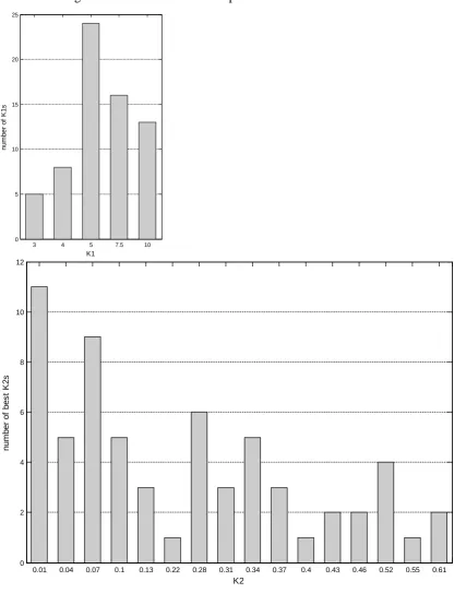
To get an overview we performed simulation runs for all product mixes with all k1 and

k2combinations. The histograms in figure 4 show how often which setting leads to the

0 0.1 0.2 0.3 0.4 0.5 0.6 0.7

950 960 970 980 990 1000 1010 1020 1030 tar di nes s [ m in] K2

0 0.1 0.2 0.3 0.4 0.5 0.6 0.7

best scheduling results over all 66 different product mixes.

Figure 4. Histogram for k1 and k2

As can be seen, the best settings, especially for k2, vary widely and corresponding

tardiness levels are highly different.

4.2 Static analysis of the machine learning quality

Especially with more product types and more settings for k1 and k2 the number of

necessary simulation runs increases quickly. Therefore, machine learning techniques

3 4 5 7.5 10

0 5 10 15 20 25

num

ber

of

K

1s

K1

0.01 0.04 0.07 0.1 0.13 0.22 0.28 0.31 0.34 0.37 0.4 0.43 0.46 0.52 0.55 0.61 0

2 4 6 8 10 12

num

ber

of

bes

t K

2s

can be used to calculate estimates for parameter combinations that have not been

simulated before. In this study, we have 66 product mix combination with 8 settings for

k1and 21 different settings for k2 leading to 11088 simulation runs with 20 replications

each. We selected different numbers of these data points between 250 and 1000 with an

LHS (latin hypercube sampling) design (McKeay, Beckman and Conover, 1979) to

calculate Gaussian process regression models and understand the benefit of more

training data. The LHS is a statistical method for generating a sample of plausible

collections of parameter values. We use it in this context to select parameter

combinations, which we simulate. The Gaussian process regression models are used to

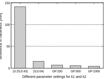
estimate the best settings for k1 and k2 for each product mix. The difference to the best

possible setting, i.e., always choosing the best k1 and k2 in each situation, is depicted in

Figure 5.

Figure 5. Learning quality of GP models constant settings compared to always using the

optimal setting

The best constant setting for all product mix combinations is k1=5 and k2=0.04. Since

these best settings would be difficult to find in scenarios where the occurring product

mixes are not known in advance, we also selected a parameter setting leading to a

performance closest to the average results of all parameter combinations. If the best

(0.25;0.43) (5;0.04) GP 250 GP 500 GP 1000

0 50 100 150

di

ff

er

enc

e i

n t

ar

di

nes

s

[

m

in]

settings are unknown and parameters are randomly taken out the reasonable range, on

average we would get the results of the combination k1=0.25 and k2=0.43. The

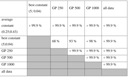
significance levels are depicted in table 1. It can be seen that the GP models perform

better than the best constant setting and clearly better than the average setting.

Table 1. Significance levels calculated with Wilcoxon test, indicating that column

method is better than row method

best constant

(5; 0.04) GP 250 GP 500 GP 1000 all data

average

constant

(0.25;0.43)

+ 99.9 % + 99.9 % + 99.9 % + 99.9 % + 99.9 %

best constant

(5;0.04) 68 % 93 % + 98 % + 99.9 %

GP 250 + 99.9 % + 99.9 % + 99.9 %

GP 500 + 99.9 % + 99.9 %

GP 1000 + 99.9 %

all data

The results are promising and demonstrate the high quality of the learned models. A

larger training set leads to significantly better accuracy, but in absolute terms the

differences are relatively small (figure 5). The selection of best settings for each product

mix leads to lower tardiness compared a constant setting. The effects and the

application of the GP models on a dynamic scenario are investigated in the following

chapter.

4.3 Dynamic simulation and system status estimation

Since the preliminary simulation runs show (figure 3) that the best constant settings for

k1 and k2 strongly depends on the product mix, we want to determine the effect in

adjusted frequently depending on the current product mix, tardiness should be lower

compared to fixed settings. Parameters can be set only if the current system status (i.e.,

product mix) is known. Therefore, we estimate the current product mix at every

machine queue, every time it completes an operation by analyzing the historic data of

the last day of operation at this machine.

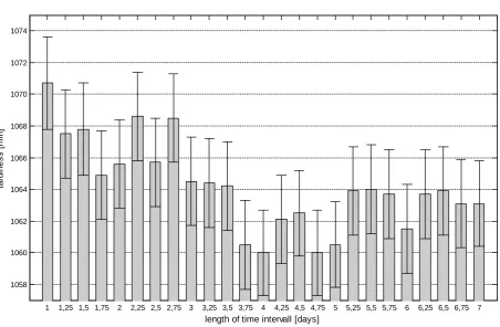
We consider the same flow shop scenario from our static preliminary simulation runs. A

suitable time span to look back is determined by a dynamic simulation study where the

product mix changes over time. Setting this look back period to a large value leads to a

(potentially too) slow reaction to changes in the product mix, setting it too short results

in frequent changes caused by random fluctuations. We select two product mixes, PM1

= [0.4, 0.4, 0.2] and PM2 = [0.8, 0.2, 0], which have different best k1 and k2values and

switch between them after 35 (PM1) and 145 (PM2) days. In 12 months this leads to 3

mix changes. As long as these periods are significantly longer than the look back

period, each period’s length can be selected arbitrarily. The data generated by the

preliminary simulation runs is used to dynamically set the ATCS parameters. The

results of this simulation study are shown in figure 6. The variance is relatively high

since the actual tardiness values are close. This means that the approach is insensitive to

the look-back period, but since the setting with 4 days performed best, we select this for

the simulation runs in our studies. A setting of 4 days represents about 3 times the mean

Figure 6. Maximum look back setting in days for estimating the product mix on a

machine (with standard error)

4.3.1 Comparison between static parameter selection and dynamic switching

To evaluate our approach we select three different dynamic scenarios with changing

product mixes over 12 months to demonstrate the potential of dynamic parameter

adjustment. On each machine the rule parameters are set before each decision is made

by the rule based on the GP prediction regarding the current product mix. This means

we have a continuous adaption process instead of choosing constant parameters.

Benchmarks with best constant parameter settings for each test scenario are calculated

by simulation runs.

In the first dynamic scenario DS1 the product mix changes from [0.3, 0.4, 0.3] to [0.4,

0.6, 0.0], in DS2 it changes from [0.3, 0.5, 0.2] to [0.6, 0.4, 0.0] and from [0.4, 0.4, 0.2]

to [0.8, 0.2, 0.0] in DS3. The product mix changes after 40 days and back after 140

days, i.e., twice during a 12 months setting. The best benchmark settings for these

scenarios are depicted in table 2, showing the best constant parameter settings for each

scenario. If all three scenarios are run sequentially the best constant parameter settings

are k1=10 and k2=0.31.

Table 2. Dynamic scenarios

1 1,25 1,5 1,75 2 2,25 2,5 2,75 3 3,25 3,5 3,75 4 4,25 4,5 4,75 5 5,25 5,5 5,75 6 6,25 6,5 6,75 7 1058

1060 1062 1064 1066 1068 1070 1072 1074

tar

di

nes

s

[

m

in]

Product mix 1 Product mix 2 Best constant

parameters

DS1 [0.3, 0.4, 0.3] [0.4, 0.6, 0.0] k1=4 k2=0.07

DS2 [0.3, 0.5, 0.2] [0.6, 0.4, 0.0] k1=10 k2=0.34

DS3 [0.4, 0.4, 0.2] [0.8, 0.2, 0.0] k1=7.5 k2=0.37

Without any prior knowledge, i.e., simulation runs that provide the best settings for one

specific scenario, one could randomly select a combination out of the reasonable range

for k1 and k2. Therefore, we performed simulation runs for all k1 and k2 combinations

and calculated the average tardiness out of these runs, which gives a mean value for

random parameter selection.

The results of simulating the selected scenarios are shown in Figure 7 and Table 3. For

each training data set size 25 different latin hypercube designs are selected. Our

experiments showed significant improvements of over 5 % using our dynamic

adjustment approach compared to the best overall setting of k1=10 and k2=0.31 and

random (4; 0.07) (10; 0.34) (7.5; 0.37) (10; 0.31) GP 50 GP 100 GP 150 GP 200 GP 250 all data 1220

1240 1260 1280 1300 1320 1340 1360

tar

di

nes

s

[

m

in]

[0.3 0.4 0.3] - [0.4 0.6 0.0]

random (4; 0.07) (10; 0.34) (7.5; 0.37) (10; 0.31) GP 50 GP 100 GP 150 GP 200 GP 250 all data 1180

1200 1220 1240 1260 1280 1300 1320 1340

tar

di

nes

s

[

m

in]

Figure 7. Results with dynamically adjusted k1andk2 values based on Gaussian process

models with different sizes of learning data sets in three scenarios (error bars indicate

twice standard error over lhs designs and random settings).

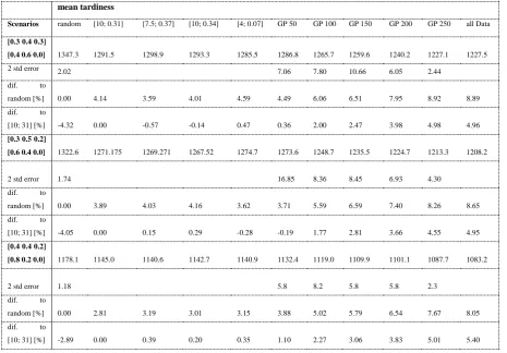
Table 3. Results of dynamic simulation runs

mean tardiness

Scenarios random [10; 0.31] [7.5; 0.37] [10; 0.34] [4; 0.07] GP 50 GP 100 GP 150 GP 200 GP 250 all Data

[0.3 0.4 0.3]

[0.4 0.6 0.0] 1347.3 1291.5 1298.9 1293.3 1285.5 1286.8 1265.7 1259.6 1240.2 1227.1 1227.5

2 std error _{2.02 7.06 7.80 10.66 6.05 2.44}

dif. to

random [%] 0.00 4.14 3.59 4.01 4.59 4.49 6.06 6.51 7.95 8.92 8.89 dif. to

[10; 31] [%] -4.32 0.00 -0.57 -0.14 0.47 0.36 2.00 2.47 3.98 4.98 4.96

[0.3 0.5 0.2]

[0.6 0.4 0.0] 1322.6 1271.175 1269.271 1267.52 1274.7 1273.6 1248.7 1235.5 1224.7 1213.3 1208.2

2 std error 1.74 16.85 8.36 8.45 6.93 4.30 dif. to

random [%] 0.00 3.89 4.03 4.16 3.62 3.71 5.59 6.59 7.40 8.26 8.65 dif. to

[10; 31] [%] -4.05 0.00 0.15 0.29 -0.28 -0.19 1.77 2.81 3.66 4.55 4.95

[0.4 0.4 0.2]

[0.8 0.2 0.0] 1178.1 1145.0 1140.6 1142.7 1140.9 1132.4 1119.0 1109.9 1101.1 1087.7 1083.2

2 std error 1.18 5.8 8.2 5.8 5.8 2.3

dif. to

random [%] 0.00 2.81 3.19 3.01 3.15 3.88 5.02 5.79 6.54 7.67 8.05 dif. to

[10; 31] [%] -2.89 0.00 0.39 0.20 0.35 1.10 2.27 3.06 3.83 5.01 5.40

random (4; 0.07) (10; 0.34) (7.5; 0.37) (10; 0.31) GP 50 GP 100 GP 150 GP 200 GP 250 all data

1060 1080 1100 1120 1140 1160 1180

tar

di

nes

s

[

m

in]

The results show that dynamic adjustment of ATCS parameters leads to significant

improvements compared to static settings. In our study, the best k2 values are between

0.03 and 0.67; scenarios with different setup matrices might have bigger differences

leading to higher improvements. In real world manufacturing, the improvements can

easily get higher, since it takes some effort to have optimal constant settings available.

4.3.2 Discussion and Conclusions

In this paper, we proposed a two-stage hybrid approach combining global information

based on offline simulations with local adaptive decision rules. The global information

about the current system status is used to adjust the autonomously working priority

rules. The advantage of this approach is the combination of the robustness of priority

rules, e.g., with respect to machine failures or unforeseen events, and the optimization

through the inclusion of global information. The number of necessary simulation runs to

learn general behavior can be reduced by employing a state-of-the-art machine learning

technique, Gaussian Process regression. It has been shown, that GPs are well-suited for

this type of application. Our GP models are based on parameters calculated dynamically

during the simulation runs, which simulates the behavior of a real production system

faced with a product mix changing over time.

Using a dynamic flow shop scenario with sequence dependent setup times, we are able

to improve the objective function (mean tardiness) significantly by dynamically

adjusting the ATCS rule parameters to the current system conditions. We can achieve

improvements of almost 9 % compared to a random parameter setting and over 5 % to

best constant parameter settings in our dynamic simulation study, which are usually not

known in advance. The approach is applicable to all scenarios, where dispatching rule

scheduling is applied.

In future research more product mix combinations and more complex scenarios should

be considered. If there are bottleneck machines for example, a strategy involving

different rule parameters for different machines, might be promising.

References

Adams, J., E. Balas, and D. Zawack. 1988. “The shifting bottleneck procedure for job

Aytug, H., M. A. Lawley, K. McKay, S. Mohan, and R. Uzsoy. 2005. “Executing

production schedules in the face of uncertainties: a review and some future

directions.” European Journal of Operational Research, 161(1):86–110.

Balasubramanian, H., L. Mönch, J. Fowler, M. Pfund. 2004. “Genetic algorithm based

scheduling of parallel batch machines with incompatible job families to minimize

total weighted tardiness.” International Journal of Production Research, 42:1621-1638

Blackstone, J. H., D. T. Phillips, and G.L. Hogg, 1982. “A state-of-the-art survey of

dispatching rules for manufacturing job shop operations.” International Journal of Production Research, 20(1):27–45.

Branke, J., S. E. Chick, and C. Schmidt. 2005. „New developments in ranking and

selection: an empirical comparison of the three main approaches.” Proceedings of the 2005 Winter Simulation Conference, 708–717.

Chen, J. Y., M. E. Pfund, J. W. Fowler, D. C. Montgomery, and T. E. Callarman. 2010.

“Robust scaling parameters for composite dispatching rules.” IIE Transactions, 42(11):842–853.

Chiang, T.-C. and L.-C. Fu. 2012. “Rule-based scheduling in wafer fabrication with due

date-based objectives.” Computers and Operations Research, 39(11):2820–2835. Dabbas, R. and J. Fowler. 2003. “A new scheduling approach using combined

dispatching criteria in wafer fabs.” Semiconductor Manufacturing, IEEE Transactions on, 16(3):501–510.

El-Bouri, A. 2012. “A cooperative dispatching approach for minimizing mean tardiness

in a dynamic flowshop.” Computers and Operations Research, 39(7):1305–1314. El-Bouri, A. and P. Shah. 2006. “A neural network for dispatching rule selection in a

job shop.” The International Journal of Advanced Manufacturing Technology, 31(3-4):342–349.

Gupta, A. K. and A. I. Sivakumar. 2006. “Job shop scheduling techniques in

semiconductor manufacturing.” The International Journal of Advanced Manufacturing Technology, 27:1163–1169.

Haupt, R. 1989. “A survey of priority rule-based scheduling.” OR Spektrum, 11(1):3– 16.

Heger, J., H. Bani, and B. Scholz-Reiter. 2012. „Improving production scheduling with

machine learning.” In L. Frommberger, K. Schill, and B. Scholz-Reiter, editors,

Heger, J., T. Hildebrandt, and B. Scholz-Reiter. 2013a. „Dispatching rule selection with

gaussian processes.” Central European Journal of Operations Research, 1–15. Heger, J., T. Hildebrandt, and B. Scholz-Reiter. 2013b. „Switching dispatching rules

with gaussian processes.” In Windt, K., editor, Robust Manufacturing Control, volume 1 of Lecture Notes in Production Engineering, 73–85. Springer.

Lee, Y. H., K. Bhaskara, and M. Pinedo. 1997. “A heuristic to minimize the total

weighted tardiness with sequence-dependent setups.” IIE Transactions, 29(1):45– 52.

Lee, Y. H. and M. Pinedo. 1997. “Scheduling jobs on parallel machines with

sequence-dependent setup times.” European Journal of Operational Research, 100(3):464– 474.

Mason, S. J., J. W. Fowler, and W. M. Carlyle. 2002. “A modified shifting bottleneck

heuristic for minimizing total weighted tardiness in complex job shops.” Journal of Scheduling, 5(3):247–262.

McKay, M. D., R. J. Beckman, and W.J. Conover. 1979. “A comparison of three

methods for selecting values of input variables in the analysis of output from a

computer code.” Technometrics, 21(2):239–245.

Metan, G., I. Sabuncuoglu, and H. Pierreval. 2010. “Real time selection of scheduling

rules and knowledge extraction via dynamically controlled data mining.”

International Journal of Production Research, 48:6909-6938.

Mönch, L. 2007. “Simulation-based benchmarking of production control schemes for

complex manufacturing systems.” Control Engineering Practice, 15:1381 –1393. Mönch, L., J. Zimmermann, and P. Otto. 2006. „Machine learning techniques for

scheduling jobs with incompatible families and unequal ready times on parallel

batch machines.” Engineering Applications of Artificial Intelligence, 19(3):235-245.

Monma, C. L. and C. N. Potts. 1989. “On the complexity of scheduling with batch setup

times.” Operations Research, 37(5):798–804.

Mouelhi-Chibani, W. and H. Pierreval. 2010. “Training a neural network to select

dispatching rules in real time.” Computers and Industrial Engineering, 58(2):249 – 256.

Ouelhadj, D. and S. Petrovic. 2009. “A survey of dynamic scheduling in manufacturing

Park, Y., S. Kim and Y.-H. Lee. 2000. “Scheduling jobs on parallel machines applying

neural network and heuristic rules.” Computers and Industrial Engineering, 38(1):189–202.

Pfund, M., J. W. Fowler, A. Gadkari, and Y. Chen. 2008. “Scheduling jobs on parallel

machines with setup times and ready times.” Comput. Ind. Eng., 54(4):764–782. Pfund, M. E., S.J. Mason, and J. W. Fowler. 2006. Handbook of Production Scheduling,

volume 89 of International Series in Operations Research & Management Science, chapter Semiconductor manufacturing scheduling and dispatching, pages 213–241. Springer, New York, 1st edition.

Pickardt, C. W. and J. Branke. 2011. “Setup-oriented dispatching rules - a survey.”

International Journal of Production Research, 50(20):1–20.

Pierreval, H. and N. Mebarki. 1997. “Dynamic scheduling selection of dispatching rules

for manufacturing system” International Journal of Production Research, 35:1575-1591.

Priore, P., D. de la Fuente, A. Gomez, and J. Puente. 2001. “A review of machine

learning in dynamic scheduling of flexible manufacturing systems.” AI EDAM, 15(03):251–263.

Rajendran, C. and O. Holthaus. 1999. “A comparative study of dispatching rules in

dynamic flowshops and jobshops.” European Journal of Operational Research, 116(1):156–170.

Rasmussen, C. E. 1996. “Evaluation of gaussian processes and other methods for

non-linear regression.” PhD thesis, Department of Computer Science, University of Toronto.

Rasmussen, C. E. and C. K. I. Williams. 2006. “Gaussian Processes for Machine Learning (Adaptive Computation and Machine Learning).” The MIT Press.

Rego, C. and R. Duarte. 2009. “A filter-and-fan approach to the job shop scheduling

problem.” European Journal of Operational Research, 194(3):650–662.

Scholz-Reiter, B., J. Heger, and T. Hildebrandt. 2010. „Gaussian processes for

dispatching rule selection in production scheduling.” Procceeding of the International Workshop on Data Mining Application in Government and Industry 2010 (DMAGI10) As Part of The 10th IEEE International Conference on Data Mining., 631–638.

Sun, Y. L. and Y. Yih. 1996. “An intelligent controller for manufacturing cells.”

van der Zee, D-J. Non-exhaustive family based dispatching heuristics - exploiting

variances of processing and set-up times. International Journal of Production Research, 48(13):3783–3802, 2010.

van der Zee, D-J., Gerard J.C. Gaalman, and Gert Nomden. Family based dispatching in

manufacturing networks. International Journal of Production Research, 49(23):7059–7084, 2011.

van der Zee, D-J. Family based dispatching with batch availability. International Journal of Production Research, 51(12):3643–3653, 2013.

V. Vinod and R. Sridharan. Simulation-based metamodels for scheduling a dynamic job

shop with sequence-dependent setup times. International Journal of Production Research, 47(6):1425–1447, 2009.

Williams, C. K. I. and C. E. Rasmussen. 1996. “Gaussian processes for regression.”

Advances in Neural Information Processing Systems, 8:514–520.

Zimmermann, J. and Mönch, L.. 2004. “Simulation-based assessment of